An optimal aggregation type classifier

Abstract

We introduce a nonlinear aggregation type classifier for functional data defined on a separable and complete metric space. The new rule is built up from a collection of $M$ arbitrary training classifiers. If the classifiers are consistent, then so is the aggregation rule. Moreover, asymptotically the aggregation rule behaves as well as the best of the $M$ classifiers. The results of a small simulation are reported both, for high dimensional and functional data.

Key words:Functional data; supervised classification; non-linear aggregation.

1 Introduction

Supervised classification is still one of the hot topics for high dimensional and functional data due to the importance of their applications and the intrinsic difficulty in a general setup. In particular, there is a large list of linear aggregation methods developed in recent years, like boosting ([4], [5]), random forest ([6], [1], [3]), among others. All these methods exhibit an important improvement when combining a subset of classifiers to produce a new one. Most of the contributions to the aggregation literature have been proposed for nonparametric regression, a problem closely related to classification rules, which can be obtained just by plugging in the estimate of the regression function into the Bayes rule (see for instance, [12] and [7]). Model selection (select the optimal single model from a list of models), convex aggregation (search for the optimal convex combination of a given set of estimators), and linear aggregation (select the optimal linear combination of estimators) are important contributions among a large list. Our approach is to combine, in a nonlinear way, several classifiers to construct an optimal one. We follow the ideas in Mojirsheibani [10] and [11] who introduced a combined classifier for the finite dimensional setup and showed strong consistency under someway hard to verify assumptions involving the Vapnik Chervonenkis dimension of the random partitions of the set of classifiers which are also non–valid in the functional setup. We extend the ideas to the functional setup and provide consistency results as well as rates of convergence under very mild assumptions. We also show optimality properties of the aggregated rule which exhibit a good behavior in high dimensional and functional data. Very recently, Biau et al. [2] introduced a new nonlinear aggregation strategy for the regression problem called COBRA, extending the ideas in Mojirsheibani [10] to the more general setup of nonparametric regression. See also [8] for some related ideas regarding density estimation.

In section 2 we introduce the new classifier in the general context of a separable and complete metric space which combines, in a nonlinear way, the decision of $M$ experts (classifiers). A more flexible rule is also considered. In Section 3 we state our two main results regarding consistency, rates of convergence and asymptotic optimality of the classifier. Asymptotically, the new rule performs as the best of the $M$ classifiers used to build it up. Section 4 is devoted to show through some simulations the performance of the new classifier in high dimensional and functional data for moderate sample sizes. All proofs are given in the Appendix.

2 The setup

Throughout the manuscript $\mathcal{F}$ will denote a separable and complete metric space, $(X,Y)$ a random pair taking values in $\mathcal{F}\times\{0,1\}$ and by $\mu$ the probability measure of $X$. The elements of the training sample $\mathcal{D}_{n}=\{(X_{1},Y_{1}),\dots,(X_{n},Y_{n})\}$, are iid random elements with the same distribution as the pair $(X,Y)$. The regression function is denoted by $\eta(x)=\mathbb{E}(Y|X=x)=\mathbb{P}(Y=1|X=x)$, the Bayes rule by $g^{*}(x)=\mathbb{I}_{\{\eta(x)>1/2\}}$ and the optimal Bayes risk by $L^{*}=\mathbb{P}\big{(}g^{*}(X)\neq Y\big{)}$.

In order to define our classifier, we split the sample $\mathcal{D}_{n}$ into two subsamples $\mathcal{D}_{k}=\big{\{}(X_{1},Y_{1}),\dots,(X_{k},Y_{k})\big{\}}$ and $\mathcal{E}_{l}=\big{\{}(X_{k+1},Y_{k+1}),\dots,(X_{n},Y_{n})\big{\}}$ with $l=n-k\geq 1$. With $\mathcal{D}_{k}$ we build up $M$ classifiers $g_{mk}:\mathcal{F}\rightarrow\{0,1\}$, $m=1,\dots,M$ which we place in the vector $\mathbf{g_{k}}(x)\doteq\big{(}g_{1k}(x),\dots,g_{Mk}(x)\big{)}$ and, following some ideas in [10], with $\mathcal{E}_{l}$ we construct our aggregate classifier as follows,

$$g_{T}(x)=\mathbb{I}_{\{T_{n}(\mathbf{g_{k}}(x))>1/2\}},$$ (1)

where

$$T_{n}(\mathbf{g_{k}}(x))=\sum_{j=k+1}^{n}W_{n,j}(x)Y_{j},\quad x\in\mathcal{F},$$ (2)

with weights $W_{n,j}(x)$ given by

$$W_{n,j}(x)=\frac{\mathbb{I}_{\{\mathbf{g_{k}}(x)=\mathbf{g_{k}}(X_{j})\}}}{\sum_{i=k+1}^{n}\mathbb{I}_{\{\mathbf{g_{k}}(x)=\mathbf{g_{k}}(X_{i})\}}}.$$ (3)

Here, $0/0$ is assumed to be $0$.

For $0\leq\alpha<1$ a more flexible version of the classifier, called $g_{T}(x,\alpha)$, can be defined replacing the weights in (3) by

$$W_{n,j}(x)=\frac{\mathbb{I}_{\{\frac{1}{M}\sum_{m=1}^{M}\mathbb{I}_{\{g_{mk}(x)=g_{mk}(X_{j})\}}\geq 1-\alpha\}}}{\sum_{i=k+1}^{n}\mathbb{I}_{\{\frac{1}{M}\sum_{m=1}^{M}\mathbb{I}_{\{g_{mk}(x)=g_{mk}(X_{i})\}}\geq 1-\alpha\}}}.$$ (4)

More precisely, the more flexible version of the classifier (1) is given by

$$g_{T}(x,\alpha)=\mathbb{I}_{\{T_{n}(\mathbf{g_{k}}(x),\alpha)>1/2\}},$$ (5)

where $T_{n}(\mathbf{g_{k}}(x),\alpha)$ is defined as in (2) but with the weights given by (4). Observe that if we choose $\alpha=0$ in (4) and (5) we obtain the weights given in (3) and the classifier (1) respectively.

Remark 1.

• The type of nonlinear aggregation used to define our classifiers turns out to be quite natural. Indeed, we give a weight different from zero to those $X_{j}$ which classify $x$ in the same group as the whole set of classifiers $\mathbf{g_{k}}(X_{j})$ (or $100(1-\alpha)\%$ of them).

• Since we are using the inverse functions of the classifiers $g_{mk}$, observations which are far from $x$ for which the condition mentioned in a) is fulfilled are involved in the definition of the classification rule. This may be very important in the case of high dimensional data. This is illustrated in figure 1.

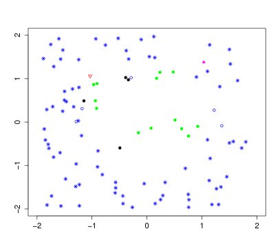
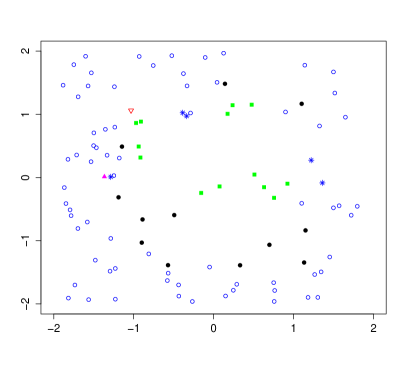
Figure 1: An example in $\mathbb{R}^{2}$ where, in both pictures, the voters of the red empty interior triangle $\nabla$ are shown as green squares while the voters of the filled magenta triangle $\Delta$ are shown with blue asterisks. The 0-class points that do not vote are shown as black dots and the 1-class points that do not vote are shown as blue circles.

3 Asymptotic results

In this section we show two asymptotic results for the nonlinear aggregation classifier $g_{T}(X,\alpha)$ (which in particular include the corresponding result for $g_{T}(X)$, taking $\alpha=0$). The first one shows that the classifier $g_{T}(X,\alpha)$ is consistent if, for $0\leq\alpha<0.5$, at least $R\geq(1-\alpha)M$ of them are consistent classifiers. Moreover, rates of convergence for $g_{T}(X,\alpha)$ (and $g_{T}(X)$) are obtained assuming we know the rates of convergence of the $R$ consistent classifiers. The second result, shows that $g_{T}(X,\alpha)$ (and in consequence $g_{T}(X)$) behaves asymptotically as the best of the $M$ classifiers used to build it up. In particular, this implies that if only one of the $M$ classifiers is consistent, then our rule is also consistent. To obtain this second result, we require a slightly stronger condition than the one used for the first result. Throughout this section we will use the notation $\mathbb{P}_{\mathcal{D}_{k}}(\cdot)=\mathbb{P}(\cdot|\mathcal{D}_{k})$.

Theorem 1.

Assume that for every $m=1,\ldots,R$ the classifier $g_{mk}$ converges in probability to $g^{*}$ as $k\to\infty$, with $R\geq M(1-\alpha)$ and $\alpha\in[0,1/2)$. Let us assume that $\mathbb{P}(Y=1|g^{*}(X)=1)>1/2$ and $\mathbb{P}(Y=0|g^{*}(X)=0)>1/2$, then

• $\lim_{min\{k,l\}\rightarrow\infty}\mathbb{P}_{\mathcal{D}_{k}}(g_{T}(X,\alpha)\neq Y)-L^{*}=0.$

• Let $\beta_{mk}\rightarrow 0$ as $k\to\infty$, for $m=1,\dots,R$ and $\bm{\beta_{Rk}}=\max_{m=1,\dots,R}\beta_{mk}$. If $\mathbb{P}_{\mathcal{D}_{k}}\big{(}g^{*}(X)\neq g_{mk}(X)\big{)}=\mathcal{O}(\beta_{mk})$, then, for $k$ large enough,

  $$\mathbb{P}_{\mathcal{D}_{k}}(g_{T}(X,\alpha)\neq Y)-L^{*}=\mathcal{O}\Big{(}\max\big{\{}\exp(-C(n-k)),\bm{\beta_{Rk}}\big{\}}\Big{)},$$

  for some constant $C>0$.

In order to state the optimality result we introduce some additional notation. Let $\mathbb{C}\doteq\{0,1\}^{M}$. For $\nu\in\mathbb{C}$ we define the following subsets

$$A_{\nu}^{0}\doteq\bigcap_{m=1}^{M}g_{mk}^{-1}(\nu(m))\cap\{Y=0\},\hskip 8.5359ptA_{\nu}^{1}\doteq\bigcap_{m=1}^{M}g_{mk}^{-1}(\nu(m))\cap\{Y=1\},$$

$$\text{ and }\hskip 2.84544ptA_{\nu}=A_{\nu}^{0}\cup A_{\nu}^{1}.$$

For each $\nu\in\mathbb{C}$, we assume that

$$(\mathcal{H})\hskip 56.9055pt\mathbb{P}_{\mathcal{D}_{k}}\big{(}(X,Y)\in A_{\nu}^{1}\big{)}\neq\mathbb{P}_{\mathcal{D}_{k}}\big{(}(X,Y)\in A_{\nu}^{0}\big{)}\hskip 8.5359pt\text{with probability one}.$$

Theorem 2.

Under assumption ($\mathcal{H}$) we have,

$$\lim_{l\to\infty}\mathbb{P}_{\mathcal{D}_{k}}\big{(}g_{T}(X,\alpha)\neq Y\big{)}\leq\mathbb{P}_{\mathcal{D}_{k}}\big{(}g_{mk}(X)\neq Y\big{)},$$

for each $m=1,\ldots,M$ which implies that,

$$\lim_{l\to\infty}\mathbb{P}_{\mathcal{D}_{k}}\big{(}g_{T}(X,\alpha)\neq Y\big{)}\leq\min_{1\leq m\leq M}\mathbb{P}_{\mathcal{D}_{k}}\big{(}g_{mk}(X)\neq Y\big{)}.$$

4 A small simulation study

In this section we present the performance of the aggregated classifier in two different scenarios. The first one corresponds to high dimensional data, while in the second one we consider two simulated models for functional data analyzed in [9].

High dimensional setting

In this setting we show the performance of our method by analyzing data generated in $\mathbb{R}^{150}$ in the following way: we generate $N$ iid uniform random variables in $[0,1]$, say $Z_{1},\ldots,Z_{N}$. For each $i=1,\ldots,N$, if $Z_{i}>1/6$, we generate a random variable $X_{i}\in\mathbb{R}^{150}$ with uniform distribution in $[-2,2]^{150}$ and $Y_{i}=1$. If $Z_{i}\leq 1/6$, we generate a random variable $X_{i}\in\mathbb{R}^{150}$ with uniform distribution in $\tau_{v}([-2,2]^{150})$ where $\tau_{v}$ is the translation along the direction $(v,\dots,v)\in\mathbb{R}^{150}$ for $v=1/4$ and set $Y_{i}=0$. Then we split the sample into two subsamples: with the first $n=N/2$ pairs $(X_{i},Y_{i})$, we build the training sample, with the remaining $N/2$ we build the testing sample.

We consider $M$ nearest neighbor classifiers with the number of neighbors taken as follows:

1. we fix $M=8$ consecutive odd numbers;

2. we choose at random $M=10$ different odd integers between $1$ and
   $\min\{\sum_{i=1}^{k}Y_{i},k-\sum_{i=1}^{k}Y_{i}\}$.

For different sizes of $N$, $k$, $l$ and $\alpha$, we build up our classifier. In Table 1, we report the misclassification errors for case 1 when compared with the nearest neighbor rules build up with a sample size $n$ taking $5,7,9,11,13,15,17,19$ nearest neighbors (these classifiers are denoted by $g_{mk}$ for $m=1,\dots,8$). The errors are shown in brackets for a sample size $k$. In Table 2, we report the misclassification errors for case 2 and compare with the (optimal) cross validated nearest neighbor classifier.

n (k)	$g_{T}(\cdot)$	$g_{T}(\cdot,1/4)$	$g_{1k}$	$g_{2k}$	$g_{3k}$	$g_{4k}$	$g_{5k}$	$g_{6k}$	$g_{7k}$	$g_{8k}$
400	.046	.056	.071	.067	.066	.067	.068	.069	.071	.073
(300)			(.074)	(.072)	(.072)	(.073)	(.074)	(.077)	(.080)	(.082)
600	.043	.052	.067	.062	.061	.061	.061	.062	.063	.065
(400)			(.072)	(.069)	(.068)	(.068)	(.069)	(.071)	(.073)	(.076)
800	.037	.045	.062	.057	.055	.055	.055	.056	.056	.057
(600)			(.066)	(.061)	(.060)	(.060)	(.060)	(.061)	(.062)	(.064)
1000	.035	.043	.061	.055	.053	.052	.052	.052	.053	.054
(700)			(.065)	(.060)	(.058)	(.057)	(.057)	(.058)	(.059)	(.060)

Table 1: Misclassification error over $500$ for $\mathbb{R}^{150}$ with fixed number of neighbors.

n	k	$g_{T}(\cdot)$	$g_{T}(\cdot,1/8)$	$g_{T}(\cdot,1/4)$	$gcv_{n}$	$gcv_{k}$
400	300	.052	.065	.077	.068	.073
600	400	.049	.063	.074	.061	.068
800	500	.048	.062	.073	.056	.061
1000	700	.047	.061	.072	.053	.058

Table 2: Misclassification error over $500$ repetitions for $\mathbb{R}^{150}$ with the number of neighbors chosen at random.

Functional data setting

In this setting we show the performance of our method by analyzing the following two models considered in [9]:

• Model I: We generate two samples of size $n/2$ from different populations following the model

  $$X_{pi}(t)=\sum_{j=1}^{6}\mu_{p,j}\phi_{j}(t)+e_{pi}(t),\hskip 28.45274ptp=1,2,\hskip 14.22636pti=1,\ldots,n/2,$$

  where $\phi_{j}(t)=\sqrt{2}\sin(\pi jt)$, $\mu_{1,j}$ and $\mu_{2,j}$ are, respectively, the j-th coordinate of the mean vectors $\mu_{1}=(0,-0.5,1,-0.5,1,-0.5)$, and $\mu_{2}=(0,-0.75,0.75,-0.15,1.4,0.1)$ while the errors are given by

  $$e_{pi}(t)=\sum_{j=1}^{40}\sqrt{\theta_{j}}Z_{pj}\phi_{j}(t),\hskip 28.45274ptp=1,2,$$

  with $Z_{pj}\sim\mathcal{N}(0,1)$ and $\theta_{j}=1/j^{2}$.

• Model II: We generate two samples of size $n/2$ from different populations following the model

  $$X_{pi}(t)=\sum_{j=1}^{3}\mu_{p,j}\phi_{j}(t)+e_{pi}(t),\hskip 28.45274ptp=1,2,\hskip 14.22636pti=1,\ldots,n/2,$$

  where $\mu_{1}=0.75\cdot(1,-1,1)$ and $\mu_{2,j}$ the j-th coordinate of $\mu_{2}\equiv 0$, $\theta_{j}=1/j^{2}$ and the errors are given by

  $$e_{pi}(t)=\sum_{j=1}^{40}\sqrt{\theta_{j}}Z_{pj}\phi_{j}(t),\hskip 28.45274ptp=1,2,$$

  with $Z_{pj}\sim\mathcal{N}(0,1)$ and $\theta_{j}=\exp\{-(2.1-(j-1)/20)^{2}\}$.

  This second model looks more challenging since although the means of the two populations are quite different, the error process is very wiggly, concentrated in high frequencies (as shown in Figure 2 left and right panel, respectively). So in this case, in order to apply our classification method, we have first performed the Nadaraya-Watson kernel smoother (taking a normal kernel) to the training sample with different values of the bandwidths for each of the two populations. The values for the bandwidths were chosen via cross-validation with our classifier, varying the bandwidths between $.1$ and $.7$ (in intervals of length $.05$). The optimal values, over 200 repetitions, were $h_{1}=.15$ for the first population (with mean $\mu_{1}$) and $h_{2}=.7$ for the second one. Finally, we apply the classification method to the raw (non-smoothed) curves of the testing sample.

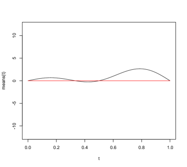
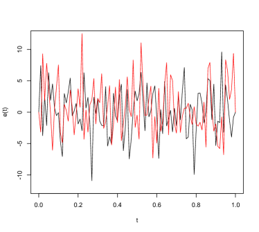
Figure 2: Mean curve (Left) and Error curve (Right) of the two populations of Model II.

In Table 3 we report the misclassification error over $200$ replications for models I and II, taking different values for $n$, $k$, $l$ and $\alpha$. In the whole training sample (of $n$ functions) the $n/2$ labels for every population were chosen at random. The test sample consist of $200$ data, taking $100$ of every population. Here, $g_{mk}=(2m-1)$-nearest neighbor rule for $m=1,\dots,5$.

Model	n (k)	$g_{T}(\cdot)$	$g_{T}(\cdot,1/5)$	$g_{T}(\cdot,2/5)$	$g_{1k}$	$g_{2k}$	$g_{3k}$	$g_{4k}$	$g_{5k}$
I	30	.005	.010	.014	.032	.015	.009	.008	.006
	(20)				.043	.024	.019	.018	.020
	50	.003	.006	.008	.025	.010	.006	.005	.004
	(30)				.033	.016	.012	.010	.009
II	30	.060	.070	.079	.098	.074	.073	.074	.077
	(20)				.097	.081	.083	.088	.094
	50	.058	.067	.071	.105	.074	.067	.065	.067
	(30)				.097	.075	.073	.076	.080

Table 3: Misclassification error over $200$ repetitions for models I and II.

For Model I we get a better performance than the PLS-Centroid Classifier proposed by [9]. For model II PLS-Centroid Classifier clearly outperforms our classifier although we get a quite small missclassification error, just using a combination of five nearest neighbor estimates.

5 Concluding remarks

We introduce a new nonlinear aggregating method for supervised classification in a general setup built up from a family of classifiers $g_{1k},\dots,g_{Mk}$. We prove consistency, rates of convergence and a certain kind of optimality, in the sense that the nonlinear aggregation rule behaves asymptotically as well as the best one among the $M$ classifiers $g_{1k},\dots,g_{Mk}$. A small simulation study confirms the asymptotic results for moderate sample sizes. In particular it is well behaved for high–dimensional and functional data.

6 Appendix: Proof of results

To prove Theorem 1 we will need the following Lemma.

Lemma 1.

Let $f(x)$ be a classifier built up from the training sample $\mathcal{D}_{k}$ such that $\mathbb{P}_{\mathcal{D}_{k}}(f(X)\neq g^{*}(X))\rightarrow 0$ when $k\rightarrow\infty$. Then, $\mathbb{P}_{\mathcal{D}_{k}}(f(X)\neq Y)-L^{*}\rightarrow 0$.

Proof of Lemma 1.

First we write,

$$\mathbb{P}_{\mathcal{D}_{k}}\big{(}f(X)\neq Y\big{)}-L^{*} =\mathbb{P}_{\mathcal{D}_{k}}\big{(}f(X)\neq Y\big{)}-P\big{(}g^{*}(X)\neq Y\big{)}$$

$$=\mathbb{P}_{\mathcal{D}_{k}}\big{(}f(X)\neq Y,Y=g^{*}(X)\big{)}$$

$$\hskip 8.5359pt+\mathbb{P}_{\mathcal{D}_{k}}\big{(}f(X)\neq Y,Y\neq g^{*}(X)\big{)}-P\big{(}g^{*}(X)\neq Y\big{)}$$

$$=\mathbb{P}_{\mathcal{D}_{k}}\big{(}f(X)\neq g^{*}(X)\big{)}$$ (6)

$$\hskip 8.5359pt+\mathbb{P}_{\mathcal{D}_{k}}\big{(}f(X)\neq Y,Y\neq g^{*}(X)\big{)}-P\big{(}g^{*}(X)\neq Y\big{)}$$

$$=\mathbb{P}_{\mathcal{D}_{k}}\big{(}f(X)\neq g^{*}(X)\big{)}-\mathbb{P}_{\mathcal{D}_{k}}\big{(}g^{*}(X)\neq Y,f(X)=Y\big{)},$$

where in the last equality we have used that

$$P\big{(}g^{*}(X)\neq Y\big{)}=\mathbb{P}_{\mathcal{D}_{k}}\big{(}g^{*}(X)\neq Y,f(X)\neq Y\big{)}+\mathbb{P}_{\mathcal{D}_{k}}\big{(}g^{*}(X)\neq Y,f(X)=Y\big{)},$$

implies

$$\mathbb{P}_{\mathcal{D}_{k}}\big{(}g^{*}(X)\neq Y,f(X)=Y\big{)}=\mathbb{P}_{\mathcal{D}_{k}}\big{(}g^{*}(X)\neq Y,f(X)\neq Y\big{)}-P\big{(}g^{*}(X)\neq Y\big{)}.$$

Therefore, replacing in (6) we get that

$$\mathbb{P}_{\mathcal{D}_{k}}\big{(}f(X)\neq Y\big{)}-L^{*} =\mathbb{P}_{\mathcal{D}_{k}}\big{(}f(X)\neq g^{*}(X)\big{)}-\mathbb{P}_{\mathcal{D}_{k}}\big{(}g^{*}(X)\neq Y,f(X)=Y\big{)}$$

$$\leq\mathbb{P}_{\mathcal{D}_{k}}\big{(}f(X)\neq g^{*}(X)\big{)},$$ (7)

which by hypothesis converges to zero as $k\to\infty$ and the Lemma is proved. ∎

Proof of Theorem 1.

We will prove part b) of the Theorem since part a) is a direct consequence of it. By (6), it suffices to prove that, for $k$ large enough:

$$\mathbb{P}_{\mathcal{D}_{k}}(g_{T}(X,\alpha)\neq g^{*}(X))=\mathcal{O}\Big{(}\max\big{\{}\exp(-C(n-k)),\bm{\beta_{Rk}}\big{\}}\Big{)}.$$

We first split $\mathbb{P}_{\mathcal{D}_{k}}(g_{T}(X,\alpha)\neq g^{*}(X))$ into two terms,

$$\mathbb{P}_{\mathcal{D}_{k}}(g_{T}(X,\alpha)\neq g^{*}(X)) =\mathbb{P}_{\mathcal{D}_{k}}(g_{T}(X,\alpha)\neq g^{*}(X),g^{*}(X)=1)$$

$$\hskip 8.5359pt+\mathbb{P}_{\mathcal{D}_{k}}(g_{T}(X,\alpha)\neq g^{*}(X),g^{*}(X)=0)\doteq I+II.$$

Then we will prove that, for $k$ large enough, $I=\mathcal{O}\Big{(}\max\big{\{}\exp(-C_{1}(n-k)),\bm{\beta_{Rk}}\big{\}}\Big{)}$. The proof that $II=\mathcal{O}\Big{(}\max\big{\{}\exp(-C_{2}(n-k)),\bm{\beta_{Rk}}\big{\}}\Big{)}$ is completely analogous and we omit it. Finally, taking $C=\min\{C_{1},C_{2}\}$, the proof will be completed. In order to deal with term $I$, let us define the vectors

$$\mathbf{g_{Rk}}(X)=\ \big{(}g_{1k}(X),\dots,g_{Rk}(X)\big{)}\in\{0,1\}^{R},$$

$$\nu(X)=\ \Big{(}1,\dots,1,g_{(R+1)k}(X),\dots,g_{Mk}(X)\Big{)}\in\{0,1\}^{M}.$$

Then,

$$I =\mathbb{P}_{\mathcal{D}_{k}}(g_{T}(X,\alpha)\neq g^{*}(X),g^{*}(X)=1)$$

$$\leq\mathbb{P}_{\mathcal{D}_{k}}(g_{T}(X,\alpha)\neq g^{*}(X),g^{*}(X)=1,\mathbf{g_{Rk}}(X)=\mathbf{1})$$

$$\hskip 14.22636pt+\sum_{m=1}^{R}\mathbb{P}_{\mathcal{D}_{k}}(g_{T}(X,\alpha)\neq g^{*}(X),g^{*}(X)=1,g_{mk}(X)=0)$$

$$\leq\mathbb{P}_{\mathcal{D}_{k}}(g_{T}(X,\alpha)\neq g^{*}(X),g^{*}(X)=1,\mathbf{g_{Rk}}(X)=\mathbf{1})$$

$$\hskip 14.22636pt+\sum_{m=1}^{R}\mathbb{P}_{\mathcal{D}_{k}}(g^{*}(X)\neq g_{mk}(X))$$

$$\leq\mathbb{P}_{\mathcal{D}_{k}}\Big{(}T_{n}(\mathbf{g_{k}}(X),\alpha)\leq 1/2\big{|}g^{*}(X)=1,\mathbf{g_{Rk}}(X)=\mathbf{1}\Big{)}$$

$$\hskip 14.22636pt+\sum_{m=1}^{R}\mathbb{P}_{\mathcal{D}_{k}}(g^{*}(X)\neq g_{mk}(X))$$

$$\doteq I_{A}+I_{B}.$$

Observe that, conditioning to $\mathbf{g_{Rk}}(X)=\mathbf{1}$ and defining

$$Z_{j}\doteq\mathbb{I}_{\left\{\frac{1}{M}\sum_{m=1}^{M}\mathbb{I}_{\{g_{mk}(X_{j})=\nu(m)\}}\geq 1-\alpha\right\}},$$

where $\nu(m)=\nu(X)(m)$ is the $m$-th entry of the vector $\nu(X)$, we can rewrite $T_{n}(\mathbf{g_{k}}(X),\alpha)$ as

$$T_{n}(\mathbf{g_{k}}(X),\alpha)=\frac{\sum_{j=k+1}^{n}Z_{j}Y_{j}}{\sum_{i=k+1}^{n}Z_{i}}.$$

Therefore,

$$I_{A} =\mathbb{P}_{\mathcal{D}_{k}}\left(\frac{\frac{1}{n-k}\sum_{j=k+1}^{n}Z_{j}Y_{j}}{\frac{1}{n-k}\sum_{i=k+1}^{n}Z_{i}}\leq\frac{1}{2}\Big{|}g^{*}(X)=1,\mathbf{g_{Rk}}(X)=\mathbf{1}\right)$$

$$=\mathbb{P}_{\mathcal{D}_{k}}\left(\frac{1}{n-k}\sum_{j=k+1}^{n}Z_{j}(Y_{j}-1/2)\leq 0\Big{|}g^{*}(X)=1,\mathbf{g_{Rk}}(X)=\mathbf{1}\right).$$ (8)

In order to use a concentration inequality to bound this probability, we need to compute the expectation of $Z_{j}(Y_{j}-1/2)=Z_{j}Y_{j}-Z_{j}/2$. To do this, observe that

$$E(Z_{j}Y_{j})=\mathbb{P}_{\mathcal{D}_{k}}\left(\frac{1}{M}\sum_{m=1}^{M}\mathbb{I}_{\{g_{mk}(U)=\nu(m)\}}\geq 1-\alpha,V=1\right),$$

and

$$E(Z_{j})=\mathbb{P}_{\mathcal{D}_{k}}\left(\frac{1}{M}\sum_{m=1}^{M}\mathbb{I}_{\{g_{mk}(U)=\nu(m)\}}\geq 1-\alpha\right),$$

being $(U,V)$ independent of $(X,Y)$, $\mathcal{D}_{k}$ and with the same law as $(X,Y)$. Since

$$\left\{\mathbf{g_{Rk}}(U)=\mathbf{1}\right\}\subset\left\{\frac{1}{M}\sum_{m=1}^{M}\mathbb{I}_{\{g_{mk}(U)=\nu(m)\}}\geq 1-\alpha\right\}\doteq A_{\alpha},$$

we have that

$$E(Z_{j}Y_{j})-E(Z_{j})/2 =\mathbb{P}_{\mathcal{D}_{k}}(V=1|A_{\alpha})\mathbb{P}_{\mathcal{D}_{k}}(A_{\alpha})-\mathbb{P}_{\mathcal{D}_{k}}(A_{\alpha})/2$$

$$=\mathbb{P}_{\mathcal{D}_{k}}(A_{\alpha})\Big{[}\mathbb{P}_{\mathcal{D}_{k}}(V=1|A_{\alpha})-1/2\Big{]}$$ (9)

$$\geq\mathbb{P}_{\mathcal{D}_{k}}\big{(}\mathbf{g_{Rk}}(U)=1\big{)}\Big{[}\mathbb{P}_{\mathcal{D}_{k}}(V=1|A_{\alpha})-1/2\Big{]}.$$

Now, since for $m=1,\ldots,R$, $g_{mk}\to g^{*}$ in probability as $k\to\infty$,

$$\mathbb{P}_{\mathcal{D}_{k}}\left(\mathbf{g_{Rk}}(U)=\mathbf{1}\right)\to\mathbb{P}(g^{*}(U)=1)\doteq p^{*}>0.$$ (10)

On the another hand, we have that, for $k$ large enough, $\mathbb{P}_{\mathcal{D}_{k}}(V=1|A_{\alpha})>1/2$. Indeed, for $m=1,\dots,R$, let us consider the events $B_{mk}=\{g_{mk}(U)=g^{*}(U)\}$ which, by hypothesis, for $k$ large enough verify

$$\mathbb{P}\big{(}\cap_{m=1}^{R}B_{mk}\big{)}>1-\varepsilon,$$

for all $\varepsilon>0$. In particular, we can take $\varepsilon>0$ such that $\mathbb{P}(V=1|g^{*}(U)=1)(1-\varepsilon)>1/2$. This implies that

$$\mathbb{P}_{\mathcal{D}_{k}}(V=1|A_{\alpha})=\ \frac{\mathbb{P}_{\mathcal{D}_{k}}(V=1,A_{\alpha},\cap_{m=1}^{R}B_{mk})}{\mathbb{P}_{\mathcal{D}_{k}}(A_{\alpha})}$$

$$\quad+\frac{\mathbb{P}_{\mathcal{D}_{k}}(V=1,A_{\alpha},(\cap_{m=1}^{R}B_{mk})^{c})}{\mathbb{P}_{\mathcal{D}_{k}}(A_{\alpha})}$$

$$\geq\ \frac{\mathbb{P}_{\mathcal{D}_{k}}(V=1,A_{\alpha},\cap_{m=1}^{R}B_{mk})}{\mathbb{P}_{\mathcal{D}_{k}}(A_{\alpha})}$$ (11)

$$=\ \frac{\mathbb{P}_{\mathcal{D}_{k}}(V=1,A_{\alpha}\big{|}\cap_{m=1}^{R}B_{mk})}{\mathbb{P}_{\mathcal{D}_{k}}(A_{\alpha})}(1-\varepsilon).$$

Conditioning to $\cap_{m=1}^{R}B_{mk}$ the event $A_{\alpha}$ equals $C_{\alpha}$ given by

$$\left\{R\mathbb{I}_{\{g^{*}(U)=1\}}+\sum_{m=R+1}^{M}\mathbb{I}_{\{g_{mk}(U)=\nu(m)\}}\geq M(1-\alpha)\right\}\doteq C_{\alpha}.$$ (12)

However, $\alpha<1/2$ imply that $C_{\alpha}=\{g^{*}(U)=1\}$. Indeed, from the inequality $R\geq M(1-\alpha)$, it is clear that $\{g^{*}(U)=1\}\subset C_{\alpha}$. On the other hand, $R\geq M(1-\alpha)>M/2$ and $\alpha<1/2$ imply that $M-R<M/2<M(1-\alpha)$, and so the sum in the second term of (12) is at most $M-R$ and consequently, $\{g^{*}(U)=1\}^{c}\subset C_{\alpha}^{c}$. Then, combining this fact with (6) we have that, for $k$ large enough

$$\mathbb{P}_{\mathcal{D}_{k}}(V=1|A_{\alpha}) \geq\ \frac{\mathbb{P}_{\mathcal{D}_{k}}(V=1,g^{*}(U)=1\big{|}\cap_{m=1}^{R}B_{mk})}{\mathbb{P}_{\mathcal{D}_{k}}(g^{*}(U)=1)}(1-\varepsilon)$$

$$=\ \frac{\mathbb{P}_{\mathcal{D}_{k}}(V=1,g^{*}(U)=1)}{\mathbb{P}_{\mathcal{D}_{k}}(g^{*}(U)=1)}(1-\varepsilon)$$ (13)

$$=\ \mathbb{P}(V=1|g^{*}(U)=1)(1-\varepsilon)$$

$$>1/2.$$

Therefore, from (10) and (6) in (6) we get

$$E(Z_{j}Y_{j})-E(Z_{j})/2>c>0.$$

Going back to (6), conditioning to $\nu(X)$ and using the Hoeffding inequality for $|Z_{j}(Y_{j}-1/2)|\leq 1/2$, for $k$ large enough we have

$$I_{A} =\mathbb{P}_{\mathcal{D}_{k}}\left(\frac{1}{n-k}\sum_{j=k+1}^{n}-\big{(}Z_{j}(Y_{j}-1/2)-E(Z_{j}(Y_{j}-1/2))\big{)}\geq c\Big{|}g^{*}(X)=1,\mathbf{g_{Rk}}(X)=\mathbf{1}\right)$$

$$\leq\exp\left\{-C_{1}(n-k)\right\},$$

with $C_{1}=2c^{2}$. On the another hand, by hypothesis we have

$$I_{B}=\sum_{m=1}^{M}\mathbb{P}_{\mathcal{D}_{k}}(g^{*}(X)\neq g_{mk}(X))=\mathcal{O}(\bm{\beta_{Rk}}),$$

which concludes the proof. ∎

Proof of Theorem 2.

First we write,

$$\mathbb{P}_{\mathcal{D}_{k}}\big{(}g_{T}(X,\alpha)\neq Y\big{)} =\mathbb{P}_{\mathcal{D}_{k}}\big{(}T_{n}(\mathbf{g_{k}}(X),\alpha)>1/2,Y=0\big{)}$$

$$\hskip 28.45274pt+\mathbb{P}_{\mathcal{D}_{k}}\big{(}T_{n}(\mathbf{g_{k}}(X),\alpha)\leq 1/2,Y=1\big{)}$$

$$\doteq I+II.$$

Then,

$$I =\sum_{\nu\in\mathbb{C}}\mathbb{P}_{\mathcal{D}_{k}}\big{(}T_{n}(\mathbf{g_{k}}(X),\alpha)>1/2,(X,Y)\in A_{\nu}^{0}\big{)}$$

$$=\sum_{\nu\in\mathbb{C}}\mathbb{P}_{\mathcal{D}_{k}}\left(\frac{\sharp\{j:(X_{j},Y_{j})\in A_{\nu}^{1}\}}{l}>\frac{\sharp\{j:(X_{j},Y_{j})\in A_{\nu}^{0}\}}{l},(X,Y)\in A_{\nu}^{0}\right),$$

and,

$$II =\sum_{\nu\in\mathbb{C}}\mathbb{P}_{\mathcal{D}_{k}}\big{(}T_{n}(\mathbf{g_{k}}(X),\alpha)\leq 1/2,(X,Y)\in A_{\nu}^{1}\big{)}$$

$$=\sum_{\nu\in\mathbb{C}}\mathbb{P}_{\mathcal{D}_{k}}\left(\frac{\sharp\{j:(X_{j},Y_{j})\in A_{\nu}^{1}\}}{l}\leq\frac{\sharp\{j:(X_{j},Y_{j})\in A_{\nu}^{0}\}}{l},(X,Y)\in A_{\nu}^{1}\right).$$

Therefore, since for all $\nu$, $\mathbb{P}_{\mathcal{D}_{k}}\big{(}(X,Y)\in A_{\nu}^{1}\big{)}\neq\mathbb{P}_{\mathcal{D}_{k}}\big{(}(X,Y)\in A_{\nu}^{0}\big{)}$ almost surely,

$$\lim_{l\to\infty}\mathbb{P}_{\mathcal{D}_{k}}\big{(}g_{T}(X,\alpha)\neq Y\big{)} =\sum_{\nu\in\mathbb{C}}\mathbb{I}_{\big{\{}\mathbb{P}_{\mathcal{D}_{k}}\big{(}(X,Y)\in A_{\nu}^{1}\big{)}>\mathbb{P}_{\mathcal{D}_{k}}\big{(}(X,Y)\in A_{\nu}^{0}\big{)}\big{\}}}\mathbb{P}_{\mathcal{D}_{k}}\big{(}(X,Y)\in A_{\nu}^{0}\big{)}\big{)}$$

$$+\sum_{\nu\in\mathbb{C}}\mathbb{I}_{\big{\{}\mathbb{P}_{\mathcal{D}_{k}}\big{(}(X,Y)\in A_{\nu}^{1}\big{)}<\mathbb{P}_{\mathcal{D}_{k}}\big{(}(X,Y)\in A_{\nu}^{0}\big{)}\big{\}}}\mathbb{P}_{\mathcal{D}_{k}}\big{(}(X,Y)\in A_{\nu}^{1}\big{)}\big{)}$$

$$=\sum_{\nu\in\mathbb{C}}\min\Big{\{}\mathbb{P}_{\mathcal{D}_{k}}\big{(}(X,Y)\in A_{\nu}^{1}\big{)},\mathbb{P}_{\mathcal{D}_{k}}\big{(}(X,Y)\in A_{\nu}^{0}\big{)}\Big{\}}.$$ (14)

On the other hand,

$$\noindent\mathbb{P}_{\mathcal{D}_{k}}\big{(}(g_{mk}(X)\neq Y\big{)} =\mathbb{P}_{\mathcal{D}_{k}}\big{(}g_{mk}(X)=0,Y=1\big{)}+\mathbb{P}_{\mathcal{D}_{k}}\big{(}g_{mk}(X)=1,Y=0\big{)}$$

$$=\mathbb{P}_{\mathcal{D}_{k}}\left(\bigcup_{\nu:\nu(i)=0}(X,Y)\in A_{\nu}^{1}\right)+\mathbb{P}_{\mathcal{D}_{k}}\left(\bigcup_{\nu:\nu(i)=1}(X,Y)\in A_{\nu}^{0}\right)$$

$$=\sum_{\nu:\nu(i)=0}\mathbb{P}_{\mathcal{D}_{k}}\big{(}(X,Y)\in A_{\nu}^{1}\big{)}+\sum_{\nu:\nu(i)=1}\mathbb{P}_{\mathcal{D}_{k}}\big{(}(X,Y)\in A_{\nu}^{0}\big{)}$$

$$\geq\sum_{\nu\in\mathbb{C}}\min\Big{\{}\mathbb{P}_{\mathcal{D}_{k}}\big{(}(X,Y)\in A_{\nu}^{1}\big{)},\mathbb{P}_{\mathcal{D}_{k}}\big{(}(X,Y)\in A_{\nu}^{0}\big{)}\Big{\}}.$$ (15)

Therefore, from (6) and (6), for each $m$ we get

$$\lim_{l\to\infty}\mathbb{P}_{\mathcal{D}_{k}}\big{(}g_{T}(X,\alpha)\neq Y\big{)}\leq\mathbb{P}_{\mathcal{D}_{k}}\big{(}g_{mk}(X)\neq Y\big{)}.$$

∎

References

References

- [1] Biau, G., Devroye, L. and Lugosi, G. (2008) Consistency of random forests and other averaging classifiers. Journal of Machine Learning Research 9 2015–2033
- [2] Biau. G, Fischer, A. Guedj, B. and Malley, J. (2013). COBRA: A Nonlinear Aggregation Strategy, arXiv:1303.2236.
- [3] Biau, G. (2012). Analysis of a random forests model. Journal of Machine Learning Research, 13 1063–1095.
- [4] Breiman, L. (1996) Bagging predictors. Machine Learning, 24:123–140.
- [5] Breiman, L. (1998) Arcing classifiers. The Annals of Statistics, 24:801–849.
- [6] Breiman, L . Random forests. Machine Learning, 45:5–32.
- [7] Bunea, F., Tsybakov, A. B. and Wegkamp, M. H. (2007). Aggregation for gaussian regression. The Annals of Statistics, 35 1674–1697.
- [8] Fraiman, R. , Liu, R. and Meloche, J. Multivariate density estimation by probing depth. –Statistical Procedures and Related Topics. IMS Lectures Notes - Monograph series (1997) Vol 31, 415–430.
- [9] Delaigle, A. and Hall. P. Journal of the Royal Statistical Society: Series B (Statistical Methodology). Volume 74, Issue 2, pages 267 1 7286, March 2012.
- [10] Mojirsheibani, M. (1999) Combining classifiers via discretization. Journal of the American Statistical Association, 94, 600–609.
- [11] Mojirsheibani, M. (2002) An almost surely optimal combined classification rule. Journal of Multivariate Analysis, 81, 28–46.
- [12] Yang, Y. (2004). Aggregating regression procedures to improve performance. Bernoulli, 10 25–47