Homogenization of Composite Ferromagnetic Materials
Abstract
Nowadays, nonhomogeneous and periodic ferromagnetic materials are the subject of a growing interest. Actually such periodic configurations often combine the attributes of the constituent materials, while sometimes, their properties can be strikingly different from the properties of the different constituents. These periodic configurations can be therefore used to achieve physical and chemical properties difficult to achieve with homogeneous materials. To predict the magnetic behavior of such composite materials is of prime importance for applications.
The main objective of this paper is to perform, by means of -convergence and two-scale convergence, a rigorous derivation of the homogenized Gibbs-Landau free energy functional associated to a composite periodic ferromagnetic material, i.e. a ferromagnetic material in which the heterogeneities are periodically distributed inside the ferromagnetic media. We thus describe the -limit of the Gibbs-Landau free energy functional, as the period over which the heterogeneities are distributed inside the ferromagnetic body shrinks to zero.
1 Introduction
Composite materials are an important class of natural or engineered heterogeneous media, composed of a mixture of two or more constituents with significantly different physical or chemical properties, firmly bonded together, which remain separate and distinct within the finished structure. Finding a model which considers the composite as a bulk and whose coefficients and terms are computed from suitable averages of those of its constituents and the geometry of the microstructure is the aim of homogenization theory. The study of composites and their homogenization is a subject with a long history, which has attracted the interest and the efforts of some of the most illustrious names in science [22]: In 1824, Poisson, in his first Mémoire sur la théorie du magnétisme [28], put the basis of the theory of induced magnetism assuming a model in which the body is composed of conducting spheres embedded in a nonconducting material. This paper is the origin of the basic models and ideas that prevailed in the theory of heterogeneous media in almost all domains of continuum mechanics, for almost a century after its appearance [22]. We refer the reader to the papers of Markov [22] and Landauer [19] for more historical details.
Nowadays, nonhomogeneous and periodic ferromagnetic materials are the subject of a growing interest. Actually such periodic configurations often combine the attributes of the constituent materials, while sometimes, their properties can be strikingly different from the properties of the different constituents [24]. These periodic configurations can be therefore used to achieve physical and chemical properties difficult to achieve with homogeneous materials. To predict the magnetic behavior of such composite materials is of prime importance for applications [24]. From a mathematical point of view, the study of composite materials, and more generally of media which involve microstructures, is the main source of inspiration for the Mathematical Theory of Homogenization which, roughly speaking, is a mathematical procedure which aims at understanding heterogeneous materials with highly oscillating heterogeneities (at the microscopic level) via an effective model [26].
The main objective of this paper is to perform, in the framework of De Giorgi’s notion of -convergence [12] and Allaire’s notion of two-scale convergence [3] (see also the paper by Nguetseng [27]), a mathematical homogenization study of the Gibbs-Landau free energy functional associated to a composite periodic ferromagnetic material, i.e. a ferromagnetic material in which the heterogeneities are periodically distributed inside the ferromagnetic media. Compared to earlier works related to the subject (see for instance [10, 11, 14, 30]) we consider here the full Gibbs-Landau functional for mixtures of different materials in the three-dimensional space.
1.1 The Landau-Lifshitz micromagnetic theory of single-crystal ferromagnetic materials
According to Landau and Lifshitz micromagnetic theory of ferromagnetic materials (see [6, 8, 18, 23]), the states of a rigid single-crystal ferromagnet, occupying a region , and subject to a given external magnetic field , are described by a vector field, the magnetization , verifying the so-called fundamental constraint of micromagnetic theory: A ferromagnetic body is always locally saturated, i.e. there exists a positive constant such that
| (1) |
The saturation magnetization depends on the specific material and on the temperature , and vanishes above a temperature (characteristic of each crystal type) known as the Curie point. Since we will assume that the specimen is at a fixed temperature below the Curie point of the material, the value will be regarded as a material dependent function, and therefore as a constant function when working on single-crystal ferromagnets. Due to the constraint (1) in the sequel we express the magnetization under the form where is a vector field which takes its values on the unit sphere of .
Even though the magnitude of the magnetization vector is constant in space, in general it is not the case for its direction, and the observable states can be mathematically characterized as local minimizers of the Gibbs-Landau free energy functional associated to the single-crystal ferromagnetic particle (using the notation of [6, 23])
| (2) |
The first term, , called exchange energy, penalizes spatial variations of . The factor in the term is a phenomenological positive material constant which summarizes the effect of (usually very) short-range exchange interactions.
The second term, , or the anisotropy energy, models the existence of preferred directions for the magnetization (the so-called easy axes), which usually depend on the crystallographic structure of the material. The anisotropy energy density is assumed to be a non-negative even and globally lipschitz continuous function, that vanishes only on a finite set of unit vectors (the easy axes).
The third term, , is called the magnetostatic self-energy, and is the energy due to the (dipolar) magnetic field, also known in literature as the stray field, generated by . From the mathematical point of view, assuming to be open, bounded and with a Lipschitz boundary, a given magnetization generates the stray field where the potential solves:
| (3) |
In (3) we have indicated with the extension of to that vanishes outside . Lax-Milgram theorem guarantees that equation (3) possesses a unique solution in the Beppo-Levi space:
| (4) |
Eventually, the fourth term , is called the interaction energy (or Zeeman energy), and models the tendency of a specimen to have its magnetization aligned with the external field , assumed to be unaffected by variations of .
The competition of those four terms explain most of the striking pictures of the magnetization that ones can see in most ferromagnetic material [17], in particular the so-called domain structure, that is large regions of uniform or slowly varying magnetization (the magnetic domains) separated by very thin transition layers (the domain walls).
1.2 The Gibbs-Landau energy functional associated to composite ferromagnetic materials
Physically speaking, when considering a ferromagnetic body composed of several magnetic materials (i.e. a non single-crystal ferromagnet) a new mathematical model has to be introduced. In fact, as far as the ferromagnet is no more a single crystal, the material depending functions and are no longer constant on the region occupied by the ferromagnet. Moreover one has to describe the local interactions of two grains with different magnetic properties at their touching interface [1].
From a mathematical point of view, this latter requirement is usually taken into account in two different ways. Either one adds to the model a surface energy term which penalizes jumps of the magnetization direction at the interface of both grains, or, and we stick on this later on, one simply considers a strong coupling, meaning that the direction of the magnetization does not jump through an interface. We insist on the fact that only the direction is continuous at an interface while the magnitude Therefore, the natural mathematical setting for the problem turns out to be characterized by the assumption that the magnetization direction is in the “weak” Sobolev metric space , i.e. on the metric subspace of constituted by the functions constrained to take values on the unit sphere of and endowed with the metric. It is in this framework that we will conduct our work from now on.
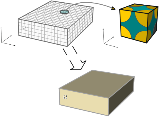
We start by recalling the basic idea of the mathematical theory of homogenization. Let be the region occupied by the composite material. If we assume that the heterogeneities are regularly distributed, we can model the material as periodic. As illustrated in Fig.1, this means that we can think of the material as being built up of small identical cubes, the side length of which being called . Let be the unit cube of . We let for be the periodic repetitions of the functions that describe how the exchange constant , the saturation magnetization and the anisotropy density energy vary over the representative cell (see Fig. 1). Substituting for , we obtain the «two-scale» functions and that oscillate periodically with period as the variable runs through , describing the oscillations of the material dependent parameters of the composite. At every scale , the energy associated to the -heterogeneous ferromagnet, will be given by the following generalized Gibbs-Landau energy functional
| (5) |
The asymptotic -convergence analysis of the family of functionals as tends to 0, is the object of the present paper.
1.3 Statement of the main result
The main purpose of this paper is to analyze, by the means of both -convergence and two-scale convergence techniques, the asymptotic behavior, as , of the family of Gibbs-Landau free energy functionals expressed by (5). Let us make the statement more precise.
We consider the unit sphere of and, for every , the tangent space of at a point will be denoted by . The class of admissible maps we are interested in is defined as
where we have denoted by the Lebesgue measure on . We consider as a metric space endowed with the metric structure induced by the classical metric. For every positive real number , we set and . We recall that a function is said to be -periodic if for every in the canonical basis of .
For the energy densities appearing in the family we assume the following hypotheses:
-
The exchange parameter is supposed to be a -periodic measurable function belonging to which is bounded from below and above by two positive constants , i.e. for -a.e. . In the setting of classical Calculus of Variations, this hypothesis guarantees that the exchange energy density, which has the form , , is a Carathéodory integrand satisfying the following quadratic growth condition for -a.e.
(6) Then we set .
-
The anisotropy density energy is supposed to be a -periodic measurable function belonging to with respect to the first variable, and globally lipschitz with respect to the second one (uniformly with respect to the first variable), i.e. such that
(7) We then set . The hypotheses assumed on are sufficiently general to treat the most common classes of crystal anisotropy energy densities arising in applications. As a sake of example, for uniaxial anisotropy, the energy density reads as
(8) the spatially dependent unit vector being the easy axis of the crystal. For cubic type anisotropy, the energy density reads as:
(9) the mutually orthogonal unit vectors being the three easy-axes of the cubic crystal. Note that the anisotropy depends on the material both in strength () and in direction ().
-
The saturation magnetization is supposed to be a -periodic measurable function belonging to , and we set .
The main result of this paper is the following:
Theorem 1.1
Let be a family of Gibbs-Landau free energy functionals satisfying the hypotheses and . Then is equicoercive in the metric space . Moreover -converges in to the functional defined by
| (10) |
The four terms that appear in (10) have the following expressions: The homogenized exchange energy is given by
| (11) |
where is the «classical» homogenized tensor given by the average
| (12) |
where for every the component is the unique (up to a constant) solution of the following scalar unit cell problem
| (13) |
The homogenized anisotropy energy is given by
| (14) |
while the homogenized magnetostatic self-energy is given by
| (15) |
where, for every , the scalar function , is the unique solution of the cell problem:
| (16) |
for all .
Finally, the homogenized interaction energy is given by
| (17) |
The paper is organized as follows: In Section 2 we give a brief survey of the main mathematical concepts and results used throughout the paper. The equicoercivity of the family is established in Section 3; the -limit of the exchange energy family of functionals is computed in Section 4; in Section 5 it is shown that the family of magnetostatic self-energies continuously converges to , while in Section 6 it is established the continuous convergence of the family of anisotropy energies to and the continuous convergence of the family of interaction energies to the functional . Eventually, the proof of mht (Theorem 1.1) is completed in Section 7, and some well-known results in homogenization theory, though somewhat difficult to find in the literature are given in the appendix.
2 Mathematical Preliminaries
The purpose of this section is to fix some notations and to give a survey of the concepts and results that are used throughout this work. All results are stated without proof as they can be readily found in the references given below.
2.1 -convergence of a family of functionals
We start by recalling De Giorgi’s notion of -convergence and some of its basic properties (see [12, 9]). Throughout this part we indicate with a metric space and, for every , with the subset of all sequences of elements of which converge to .
Definition 2.1
(-convergence of a family of functionals) Let be a sequence of functionals defined on with values on . The functional is said to be the - of with respect to the metric , if for every we have:
| (18) |
and
| (19) |
In this case we write .
If is a family of functionals, we say that is the - of as , if for every one has . In this case we write .
The condition (19) is sometimes referred to in literature as the existence of a recovery sequence.
One of the most important properties of -convergence, and the reason why this kind of variational convergence is so important in the asymptotic analysis of variational problems, is that under appropriate compactness hypotheses it implies the convergence of (almost) minimizers of a family of equicoercive functionals to the minimum of the -limit functional. More precisely, the following result holds:
Theorem 2.2
(Fundamental Theorem of -convergence) If is a family of equicoercive functionals -converging on to the functional . Then is coercive and lower semicontinuous (therefore there exists a minimizer for on ) and we have the convergence of minima values
| (20) |
Moreover, given and a converging sequence such that
| (21) |
its limit is a minimizer for on . If (21) holds, the sequence is said to be a sequence of almost-minimizers for .
Let us recall now that given two families of functional and -converging respectively to and , it is in general not the case (see [9]) that - . A sufficient condition for that property to hold is that at least one of the two families of functionals satisfies a stronger type of convergence:
Definition 2.3
We say that a family of functionals is continuously convergent in to a functional , and we will write , if for every
We then have (see [9] for a proof):
Proposition 2.4
Let . Suppose that the family of functionals continuously converges to , and that and are everywhere finite on . Then and
In particular if is a continuous functional then and is called a continuous perturbation of the -limit.
2.2 -scale convergence
The aim of this section is to present in a schematic way the main properties of two-scale convergence, a notion that is first due to Nguetseng [27], developed as a methodology by Allaire [3] and further investigated by many others (see [2] and references therein for instance).
We denote by the set of infinitely differentiable real functions over that are -periodic and define as the closure of in . Obviously any element of has the same trace on the opposite faces of .
A generalized version of the Riemann-Lebesgue Lemma holds for the weak limit of rapidly oscillating functions. For a proof we refer the reader to [13].
Proposition 2.5
Let be any open set. Let and be a positive real number. Let be a -periodic function. Set -a.e. on . Then, if , as
If , one has
Definition 2.6
Let be an open set , and let be a fixed sequence of positive real numbers (when it is clear from the context we will omit the subscript ) converging to . The sequence of functions is said to two-scale converge to a limit , if for any function we have
| (22) |
In this case we write . We say that in strongly two-scale converges to a limit if and moreover
The importance of this new notion of convergence relies on the following compactness results.
Proposition 2.7
For each bounded sequence , there exists an such that, up to a subsequence, .
Moreover, for bounded sequences in we have the following result:
Proposition 2.8
Let be a sequence in that converges weakly to a limit . Then and there exists a function such that, up to a subsequence:
Next we recall that if the sequence is bounded in , it is possible to enlarge the class of test functions used in the definition of two-scale convergence.
Proposition 2.9
Let be a bounded sequence in which two-scale converges to . Then
for every .
Finally we recall a simple criteria that permits to «bypass» the problem concerning the convergence of the product of two -weakly convergence sequences (cfr.[3, 20]).
Proposition 2.10
Let and be sequences in that respectively two-scale converge to and in . If at least one of them strongly two-scale converges, then
In particular, if is bounded in , from the previous proposition, we have
for every .
3 The equicoercivity of the composite Gibbs-Landau free energy functionals
This section is devoted to the proof of the equicoercivity of the family of Gibbs-Landau free energy functionals expressed by (5). Equicoercivity has an important role in homogenization theory. In fact, the metric space in which to work, must be able to guarantee the equicoercivity of the family of functionals under consideration, i.e. the validity of the Fundamental Theorem of -convergence.
Proposition 3.1
The family of Gibbs-Landau energy functionals is equicoercive on the metric space .
Proof 3.2
According to the hypotheses and , there exist positive constants such that for every
Therefore, for every on has
| (23) |
with .
Now observe that for every constant in space magnetization and for every on has ; thus
| (24) |
To finish, we simply observe that, due to Rellich–Kondrachov theorem, is a compact subset of .
4 The -limit of exchange energy functionals
The fundamental constraint of micromagnetic theory, i.e. the fact that the domain of definition of the family is a manifold value Sobolev space, plays a fundamental role in the homogenization process. In fact, although the unconstrained problem has been fully investigated (see [7, 21, 25]), it is not possible to get full information about the manifold constrained -limit by just looking at the unconstrained one. This is due to the well-known fact (see [9]) that if is a family of functionals defined in the metric space and -converging to , and where represents the family of functionals obtained as the restriction of to some (metric) subspace of , then . Thus the identification of the manifold constrained -limit requires more effort.
4.1 The tangential homogenization theorem
In what follows we make use of the following theorem due to Babadjian and Millot (see [5]) in which the dependence of the -limit from the tangent bundle of the manifold is taken into account via the so-called tangentially homogenized energy density. We state the tangential homogenization theorem (thm) in a bit less general form which is adequate for our purposes.
Proposition 4.1
(thm) [5] Let be a connected smooth submanifold of without boundary and be a Carathéodory function such that
-
1.
For every the function is -periodic, i.e. such that if denotes the canonical basis of , one has
-
2.
There exist such that
Then the family
| (25) |
defined in the metric space -converges to the functional
| (26) |
where for every and , ,
| (27) |
is the tangentially homogenized energy density.
We refer the reader to [5] for a more general version and the proof.
4.1.1 The role of tangent bundle.
Let us emphasize why the tangent bundle plays a role. In order to understand this, it is convenient to develop a minimizer of under the so-called multiscale expansion
| (28) |
where are respectively a minimizer of the -limit of and the null average first order corrector. Clearly, due to the constraint for a.e. , we get
| (29) |
where we have denoted by the local normal field defined around . By passing to the two-scale limit in both terms of (29), we formally reach the equality , which shows that does not depend on . Then, passing to the average over we get . The rigorous formulation of the previous idea is the object of the next Proposition:
Proposition 4.2
Let be a connected smooth submanifold of , and let be a sequence in that converges weakly to a limit . Then
Moreover there exists a null average function such that, up to the extraction of a a subsequence:
Proof 4.3
In view of Proposition 2.8, we only need to prove that for a.e. . To this end, let us denote by the normal vector at and observe that it is sufficient to prove that the scalar function does not depend on the variable, i.e. that in the language of distributions on one has
| (30) |
Indeed, as far as is independent from the variable, since by assumption for a.e. , one has and therefore for a.e. .
4.1.2 The role of tangentially homogenized energy density
Although the following considerations are not completely rigorous, they give a very good explanation of the idea behind the expression of the tangentially homogenized energy density (27); they are mainly based on the notion of two-scale convergence while [5] relies on -convergence.
Let us denote by the family of functionals
| (31) |
and let us denote by its -limit in the metric space . Since is a metric subspace of , from the properties of -convergence under restriction to subspaces (see [9]), we know that for every and for every
| (32) |
Now, let be a convex smooth manifold, i.e. a smooth manifold lying on some subset of the boundary of a convex bounded domain . Next, define the tangent cone of at by the position
and denote by the nearest point projection on .
Since is a (Lipschitz) non-expansive map, one has for every , moreover (see [4])
| (33) |
Let us now suppose that is sufficiently smooth so that for every test function , the family belongs to . In this hypothesis one has
Therefore, taking into account the estimates (33), (32) and the fact that is an admissible test function (see [3], Remark 1.11), we get (passing to the two-scale limit):
Since is an arbitrary test function, passing to the infimum we finish with the following upper and lower bound for the manifold constrained homogenized functional:
| (34) |
with
| (35) |
Since the functional is continuous with respect to the norm and is dense in , the infimum in (34) can be taken over .
4.2 The tangentially homogenized Exchange Energy
Let us go back to the application of the tangentially homogenization result in our setting. We consider the family of exchange energy functionals, all defined in , given by . Since holds, Proposition 4.1 ensures that the family -converges in the metric space , i.e. with respect to the topology induces on by the strong topology, to the functional
| (36) |
where for every and every ,
| (37) |
with
Equivalently, since is a continuous functional, and the subspace is dense in , we have for every and every
| (38) |
and hence
| (39) |
This latter formulation is a more convenient one. Indeed, it can be easily verified, by Lax-Milgram theorem, that for every , every and every , there exists a unique solution of the problem
| (40) |
Moreover, for every and every , the function
| (41) |
is a (continuous) linear map.
Let us now consider the problem that defines the classical homogenization problem (see [7, 21, 25]), namely
| (42) |
Our aim is now to prove that the natural extension of to the tangent bundle coincides with the tangentially homogenized energy density . To this end we observe that in the «classical» problem (42), the function space among which the minimization takes place is bigger than the one involved in the original problem (39), so that for every .
To prove that on it is thus sufficient to show that for every and for every there exists a function such that . Having this goal in mind, we observe that if is the unique solution of the minimization problem arising in (42), denoting by the nearest point projection of on , one has and
where, in deriving the previous equalities, we have used the relations , , and the orthogonality relations , . Thus we have
and therefore, passing to the limit for we get . In particular does not depend on , and is given by (42).
Remark 4.5
The fact that tangential homogenization energy density reduces to the «classical» one (i.e. ), which does not depend from the -variable, is a quite remarkable fact. Indeed, it is possible to build elementary examples where the dependence on the -variable in the tangential homogenization energy density is explicit (cfr. [5]). The independence from the -variable in our framework, is mainly due to the very particular situation that for every , the Carathéodory function is invariant under the rotation group of the manifold under consideration (the 2-sphere ).
To complete the proof concerning the exchange energy part stated in Theorem 1.1, it is sufficient to recall that is a quadratic form in (see [7, 21]), i.e. that there exists a symmetric and positive definite matrix such that for every
| (43) |
Precisely, it is possible to show that the «classical» problem (42) may be equivalently reformulated by replacing homogeneous boundary conditions by periodic boundary conditions (see [25] and Appendix A), so that for every
| (44) |
Furthermore, from the convexity of the integrand, it is routinely seen that we can replace the limit for by the computation on the unit cell (though still with periodic boundary conditions). We are therefore left (see [7] and Appendix A) for every with
| (45) |
Now, Lax-Milgram theorem shows that for every there exists a unique solution of this latter problem, up to an additive constant that we may fix by requiring that . Moreover, the map is a (continuous) linear map, and a direct computation, shows that can be expressed as:
| (46) |
where for every the component is the unique (up to a constant) solution of the scalar unit cell problem
| (47) |
Remark 4.6
By repeating the same argument followed above to deduce the equality , it is now simple to show that the tangentially homogenized exchange energy density can be equivalently characterized by the position
which is exactly the one deduced in equation (34).
5 The periodic homogenization of the demagnetizing field
This Section is devoted to show that the family of magnetostatic self-energies continuously converges to . To this end, let us first recall some essential facts concerning the demagnetizing field operator.
5.1 The Beppo-Levi space and the variational formulation for the demagnetizing field
From the mathematical point of view, assuming to be open, bounded and with a Lipschitz boundary, a given magnetization generates the stray field where the potential solves:
| (48) |
In (48) we have denoted by the extension of to that vanishes outside .
Once introduced the weight , and the weighted Lebesgue space
we define the Beppo-Levi space
| (49) |
which is an Hilbert space when endowed with the scalar product . It is straightforward to show, by the means of Lax-Milgram theorem, the existence and uniqueness of the solution of the variational formulation associated to equation (48): namely to find a potential such that for all
| (50) |
Thus, for every there exists a unique such that (50) holds, and moreover, the following stability estimate holds:
| (51) |
The quantity is what is referred to as the demagnetizing field, and it is a linear and continuous operator from into . In particular for every and therefore is also a linear and continuous operator from into .
5.2 The two-scale limit of the demagnetizing field
In this subsection we make use of the notion of two-scale convergence, to characterize the behavior of the demagnetizing field operator under two-scale convergence. More precisely, we suppose to have a bounded sequence which two scale converges to some and we want to understand if the two-scale limit of the sequence exists, and in the affirmative case to characterize in some analytic sense such a limit. This problem has already been treated in [30] although without justifying the use of two-scale compactness results in weighted space. That is why in this subsection we start by proving two compactness results concerning two-scale convergence in the weighted spaces and .
The first one is a «weighted» variant of the compactness result stated in Proposition 2.7, and shows that a notion of two-scale convergence in makes sense.
Proposition 5.1
Let be bounded sequence in . There exists a function such that and, up to the extraction of a subsequence,
| (52) |
for all . In this case we say that the sequence -two-scale converges to .
Proof 5.2
Since is bounded in the Hilbert space , there exists an element and a sequence such that
| (53) |
This implies that for every bounded domain , one has weakly in . We now consider a sequence of bounded domain covering . Let us start with the index , i.e. with . According to the two-scale compactness result (see Proposition 2.7), there exists a subsequence and an element such that
| (54) |
Now we consider , i.e. . Since weakly in , it is possible to extract a further subsequence from such that in for some suitable . Moreover, due to the unicity of the two-scale limit, one has
| (55) |
whenever . Proceeding in this way, we find for every a subsequence such that
| (56) |
for some . We then define the diagonal sequence of indices defined by
| (57) |
From (56) we get that for every , up to the first terms, the sequence of indices is included in , and this means that for every
| (58) |
By observing again that if , from the «principe du recollement des morceaux» (cfr. [31]) there exists a unique distribution such that , and therefore
| (59) |
for every . Moreover since
| (60) |
and
| (61) |
we get also . This completes the proof.
Exactly with the same diagonal argument, it is possible to prove the weighted variant of the compactness result stated in Proposition 2.8.
Proposition 5.3
Let be bounded sequence in weakly convergent to . Then -two-scale converges to and there exists a function such that, up to the extraction of a subsequence:
| (62) |
Proof 5.4
We start by observing that since weakly in , in , and therefore, according to the previous proposition, there exists a function such that, up to a subsequence,
| (63) |
We now consider a sequence of bounded domain . Proceeding as in the proof of the previous Proposition 5.1, one proves that for every there exists a subsequence such that
| (64) |
We then define the diagonal sequence of indices defined by the position . From (64) we get that for every , up to the first terms, the sequence of indices is included in , and this means that for every
| (65) |
Thus in .
Next, we observe that since weakly in we have and bounded in . Thus, according to the classical two-scale compactness result (see Proposition 2.8) there exists a function such that, up to a subsequence,
| (66) |
Thus, for any test function with one has
| (67) |
Passing to the two-scale convergence on both sides we get that for a.e. and for every such that in .
| (68) |
Since the orthogonal complement of the divergence-free functions is the space of gradients, for a.e. there exists a unique function such that . Thus and , i.e. . This completes the proof.
We are now ready to prove the two-scale convergence of the demagnetizing field operator (for this we follow the lines of [30]):
Proposition 5.5
Let be a bounded family in that two-scale converges to . Then the two-scale limit of exists and is given by
| (69) |
where for every the scalar function is the unique solution in of the cell problem
| (70) |
and therefore of the variational cell problem
| (71) |
for all .
Proof 5.6
Since is bounded in , due to the stability estimate (51), the sequence of magnetostatic potentials solution of the problem , remains bounded in . This means that, up to a subsequence, weakly in for some suitable . Thus, according to Proposition 5.3, there exist functions and such that
| (72) |
In view of the previous limit relations, is expected to behave as . This suggest to use, in the variational formulation of the magnetostatic problem expressed by equation (50), test functions having the form , with and . This yields
From the second of the two limit relations (72), we get
| (73) |
In particular, by choosing we get
| (74) |
where the last equality follows from the fact that . Thus, we reach the conclusion that the weak limit satisfies the variational formulation (74), i.e. is a solution of the «homogenized» equation
| (75) |
On the other hand by choosing and in (73) we get
and hence the so-called cell problem
| (76) |
where, again, the last equality follows from the fact that . Note that the variational formulation (76) can be more concisely expressed in the form
| (77) |
and the well-posedness of the previous variational problem is again a direct consequence of Lax-Milgram theorem.
5.3 The continuous limit of magnetostatic self-energy functionals
In what follows we will make use of Proposition 5.5, to prove the following
Proposition 5.7
The family of magnetostatic self-energies
| (78) |
continuously converges to the functional
| (79) |
where for every the scalar function is the unique solution of the following variational cell problem:
| (80) |
| (81) |
for all .
Proof 5.8
We know (see Proposition 2.5) that weakly∗ in . In particular, by choosing as a test function we get
and therefore strongly.
Next, since is bounded in , from Proposition 2.10 and Proposition 5.5, we get
| (82) |
Now, we observe that for every the scalar function is the unique solution of the variational cell problem (71), therefore setting in (71) we get
| (83) |
and therefore
| (84) |
Now we show that the family continuously converges to . This amounts to prove that for every and every , and implies . To this end, for every we split:
| (85) |
From (84) it follows the existence of a sufficiently small such that
| (86) |
On the other hand, since is a linear and continuous map from into with (and ) one has
| (87) |
and the previous estimate together with (86) clearly concludes the proof.
6 The homogenized anisotropy and interaction energies
This section is devoted to the proof of the continuous convergence of the family of anisotropy energy functionals and of the family of interaction energy functionals , respectively to and , whose expression is given by (14) and (17).
6.1 The continuous limit of the anisotropy energy functionals
Proposition 6.1
If the anisotropy energy density is -periodic with respect to the first variable and globally lipschitz with respect to the second one (uniformly with respect to the first variable) then the family of anisotropy energies continuously converges to the homogenized anisotropy energy
| (88) |
Proof 6.2
Again, we have to prove that for every one has
For every we split
| (89) |
Next, we observe that since weakly∗ in (cfr. Lemma 2.5), there exists a sufficiently small such that for every
| (90) |
On the other hand, by the global lipschitz continuity in the second variable of , we have
| (91) | ||||
| (92) |
Substituting estimates (90) and (92) into (89) we get
| (93) |
Therefore for every such that we get , and this concludes the proof.
Corollary 6.3
Uniaxial anisotropy energy density. If then
6.2 The continuous limit of interaction energy functionals
The convergence of to is straightforward. Indeed this energy term is expressed by the product, with respect to the scalar product, of the constant function and the weakly converging sequence weakly∗ in (cfr. Lemma 2.5). Therefore repeating the same argument given in the previous subsection:
7 Proof of Theorem 1.1 completed
It is now easy to complete the proof of Theorem 1.1. Indeed the equicoercivity of the family of Gibbs-Landau free energy functionals expressed by (5) has been proved in Section 3. It is therefore sufficient to recall the stability properties of the -limit under the sum of a continuously convergent family of functionals. In fact, what has been proved in the previous subsections, can be summarized by the following convergence scheme
| (94) |
Thus, Proposition 2.4 completes the proof.
8 Conclusions and acknowledgment
We have given in this paper a complete theory for periodic microstructured magnetic materials. Obtained through a process of convergence the model derives rigorously the energy terms from the parameters of each constituent of the sample and the mixing geometry of the different materials in the unit periodic cell. We believe that the result applies to most of magnetic composites that are nowadays considered, e.g. those obtained from a mixing of hard and soft phases [15, 32] or the multilayer magnetic materials [16, 29]. In this latter case, the formula obtained furthermore simplifies since the exchange coefficient can be analytically computed. We leave the exploration of potential applications to a forthcoming work.
Appendix A Restatement of some well-known result
In this appendix we state, in a bit general form, two results that we mentioned in the previous sections. We start with a result whose proof can be extracted from [25], which permits to pass, in the characterization of the homogenized energy density, from homogeneous boundary conditions to periodic ones. The proof, although well-known in the homogenization community, is difficult to find in the classical monographs on the subject:
Proposition A.1
Let be a vector subspace of and let be a Carathéodory function satisfying the hypotheses of (thm) with (see Proposition 4.1). Then, for every one has with
| (95) |
Proof A.2
Since it is obvious that does not depend on the -variable. Moreover, since one trivially has . Let us therefore focus on the converse inequality. For any and any we consider the family which converges to in the metric space . By the characterizing properties of the -limit we have:
| (96) |
Since the integrand in the last member of the previous equation is -periodic and satisfies the hypotheses of the generalized Riemann-Lebesgue Lemma (cfr. Proposition 2.5) we finish with the estimate
| (97) |
Passing to the infimum we get the stated result.
Finally, in the hope to achieve our goal of making the material contained in this paper accessible to as large audience as possible, we prefer to state – again in a bit general form – and give a more «commented» proof of the following well-known result (cfr. [7]) which permits, in the convex case, to pass from variations that are periodic over an ensemble of 1-cells to variations that are periodic in the unit cell .
Proposition A.3
Let be a Carathéodory integrand satisfying the hypotheses of (thm) (Proposition 4.1). If for any the function is convex, then for any convex subset of and every the following equality holds:
| (98) |
Proof A.4
One of the main ingredients of the argument, is in observing that for every the following decomposition of the -cube in -cubes holds:
| (99) |
and . Thus, from the -periodicity of in the first variable, we arrive to the intuitive and well-known fundamental equality:
| (100) |
Next, we observe that for every , and therefore, from the previous equality we get:
To complete the proof we now prove that the previous inequality is actually an equality, and therefore (in particular) that the left hand side of (98) does not depend on . To this end it is sufficient to show that for every and every there exists a such that
| (101) |
With this goal in mind, for every , we define the convex combination
| (102) |
Clearly belongs to . Moreover, by the convexity and -periodicity of with respect to the first variable, from equality (100), we get:
and this completes the proof.
References
- [1] E. Acerbi, I. Fonseca, G. Mingione. Existence and regularity for mixtures of micromagnetic materials. Proceedings of the Royal Society A: Mathematical, Physical and Engineering Science, 462.2072 (2006): 2225-2243.
- [2] G. Allaire, M. Briane. Multiscale convergence and reiterated homogenisation. Proceedings of the Royal Society of Edinburgh: Section A Mathematics, 126.02 (1996): 297-342.
- [3] G. Allaire. Homogenization and two-scale convergence. SIAM Journal on Mathematical Analysis., 23.6 (1992): 1482-1518.
- [4] F. Alouges. A new algorithm for computing liquid crystal stable configurations: the harmonic mapping case. SIAM Journal on Numerical Analysis, 34.5 (1997): 1708-1726.
- [5] J.-F. Babadjian, V. Millot. Homogenization of variational problems in manifold valued Sobolev spaces. ESAIM: Control, Optimisation and Calculus of Variations , 16.04 (2010): 833-855.
- [6] G. Bertotti. Hysteresis in magnetism: for physicists, materials scientists, and engineers. Academic press, 1998.
- [7] A. Braides, A. Defranceschi. Homogenization of Multiple Integrals. Oxford University Press, 1998.
- [8] W. F. Brown. The fundamental theorem of the theory of fine ferromagnetic particles. Annals of the New York Academy of Sciences, 147.12 (1969): 463-488.
- [9] G. Dal Maso. An introduction to -convergence. Progress in Nonlinear Differential Equations and their Applications. Birkhauser Boston, 1993.
- [10] A. De Simone. Energy minimizers for large ferromagnetic bodies. Archive for rational mechanics and analysis, 125.2 (1993): 99-143.
- [11] A. De Simone. Hysteresis and imperfections sensitivity in small ferromagnetic particles. Meccanica ,30.5 (1995): 591-603.
- [12] E. De Giorgi, T. Franzoni. Su un tipo di convergenza variazionale. Atti Accad. Naz. Lincei Rend. Cl. Sci. Fis. Mat. Natur., (8) 58.6 (1975): 842-850.
- [13] D. Cioranescu, P. Donato. An introduction to homogenization. Oxford Lecture Series in Mathematics and its Applications. Oxford University Press, 1999.
- [14] H. Haddar and P. Joly. Homogenized model for a laminar ferromagnetic medium. Proc. Roy. Soc. Edinburgh Sect. A 133.3 (2003): 567-598.
-
[15]
G. Hadjipanayis and A. Gabay.
The incredible pull of nanocomposite magnets.
IEEE Spectrum.
Available at http://spectrum.ieee.org/semiconductors/nanotechnology/the-incredi
ble-pull-of-nanocomposite-magnets. - [16] J.-G. Hu, J.-W. Liu and Y. Q. Ma. Remanence characteristic of nanostructure of Hard/Soft magnetic multilayered systems. Communication in Theoretical Physics 35 (2001): 740-744.
- [17] A. Hubert and R. Schaefer. Magnetic Domains: The Analysis of Magnetic Microstructures. Springer, 1998.
- [18] L. Landau, E. Lifshitz. On the theory of the dispersion of magnetic permeability in ferromagnetic bodies. Phys. Z. Sowjetunion , 8.153 (1935): 101-114.
- [19] R. Landauer. Electrical conductivity in inhomogeneous media AIP Conference Proceedings, 40.1 (1978): 2-45.
- [20] D Lukkassen, G. Nguetseng, P. Wall. Two-scale convergence. Int. J. Pure Appl. Math, 2.1 (2002): 35-86.
- [21] P. Marcellini. Periodic solutions and homogenization of non linear variational problems. Annali di matematica pura ed applicata, 117.1 (1978): 139-152.
- [22] K. Z. Markov. Heterogeneous media: micromechanics modeling methods and simulations. Springer 2000.
- [23] I.D. Mayergoyz, G. Bertotti, C. Serpico. Nonlinear magnetization dynamics in nanosystems. Elsevier, 2008.
- [24] G. W. Milton. The Theory of Composites. Cambridge Monographs on Applied and Computational Mathematics. Cambridge University Press, 2002.
- [25] S. Müller. Homogenization of nonconvex integral functionals and cellular elastic materials. Archive for Rational Mechanics and Analysis, 99.3 (1987): 189-212.
- [26] A. K. Nandakumaran. An overview of Homogenization. Journal of the Indian Institute of Science ,87.4 (2012): 475.
- [27] G. Nguetseng. A general convergence result for a functional related to the theory of homogenization. SIAM Journal on Mathematical Analysis, 20.3 (1989): 608-623.
- [28] S. D. Poisson. Mémoire sur la théorie du magnétisme. Mémoires de l’Académie royale des Sciences de l’Institut de France, 1826.
- [29] J. P. Renard. Magnetic multilayers. Journal of Materials Science and Technology, 9 (1993).
- [30] K. Santugini-Repiquet. Homogenization of the demagnetization field operator in periodically perforated domains. Journal of mathematical analysis and applications, 334.1 (2007): 502-516.
- [31] L. Schwartz. Théorie des distributions, volume 1. Hermann, 1957.
- [32] R. Skomski and J. M. D. Coey. Giant energy product in nanostructured two-phase magnets. Physical Review B, 48.21 (1993):15812-15816.