On existence of thermally coupled incompressible flows in a system of three dimensional pipes

Abstract

We study an initial-boundary-value problem for time-dependent flows of heat-conducting viscous incompressible fluids in a system of three-dimensional pipes on a time interval $(0,T)$. Here we are motivated by the bounded domain approach with “do-nothing” boundary conditions. In terms of the velocity, pressure and enthalpy of the fluid, such flows are described by a parabolic system with strong nonlinearities and including the artificial boundary conditions for the velocity and nonlinear boundary conditions for the so called enthalpy of the fluid. The present analysis is devoted to the proof of the existence of weak solutions for the above problem. In addition, we deal with some regularity for the velocity of the fluid.

1 Introduction

Many problems of fluid thermo-mechanics involving unbounded domains occur in many areas of applications, e.g. flows of a liquid in duct systems, fluid flows through a thin or long pipe or through a system of pipes in hemodynamics and so on. From a numerical point of view, these formulations are not convenient and quite practical. Therefore, an efficient natural way is to cut off unbounded parts of the domain by introducing an artificial boundary in order to limit the computational work. Then the original problem posed in an unbounded domain is approximated by a problem in a smaller bounded computational region with artificial boundary conditions prescribed at the cut boundaries. Hence, let $\Omega$ be a bounded domain in $\mathbb{R}^{3}$ with boundary $\partial\Omega$. In a physical sense, $\Omega$ represents a “truncated” region of an unbounded system of pipes occupied by a moving heat-conducting viscous incompressible fluid. ${\Gamma_{1}}$ will denote the “lateral” surface and ${\Gamma_{2}}$ represents the open parts (cut boundaries) of the piping system. It is physically reasonable to assume that in/outflow pipe segments extend as straight pipes. More precisely, $\Gamma_{1}$ and ${\Gamma_{2}}$ are ${C}^{\infty}$-smooth open disjoint not necessarily connected subsets of $\partial\Omega$ such that $\Gamma_{2}=\bigcup_{i\in\mathcal{J}}\Gamma^{(i)}_{2}$, $\Gamma^{(i)}_{2}\cap\Gamma^{(j)}_{2}=\emptyset$ for $i\neq j$, $\partial\Omega=\overline{\Gamma}_{1}\cup\overline{\Gamma}_{2}$, ${\Gamma_{1}}\neq\emptyset$, ${\Gamma_{2}}\neq\emptyset$, $\mathcal{M}=\partial\Omega-({\Gamma_{1}}\cup{\Gamma_{2}})=\overline{\Gamma}_{1}\cap\overline{\Gamma}_{2}=\bigcup_{i\in\mathcal{J}}\mathcal{M}_{i}$, $\mathcal{J}=\left\{1,\dots,d\right\}$, and the $2$–dimensional measure of $\mathcal{M}$ is zero and $\mathcal{M}_{i}$ are smooth nonintersecting curves (this means that $\mathcal{M}_{i}$ are smooth curved nonintersecting edges and vertices (conical points) on $\partial\Omega$ are excluded). Moreover, all portions of ${\Gamma_{2}}$ are taken to be flat and ${\Gamma_{1}}$ and ${\Gamma_{2}}$ form a right angle $\omega_{\mathcal{M}}=\pi/2$ at all points of $\mathcal{M}$ (in the sense of tangential planes), see Figure 1.

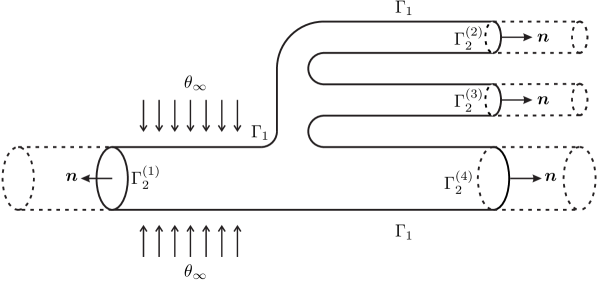
Figure 1: Truncated piping system.

The flow of a viscous incompressible heat-conducting fluid is governed by balance equations for linear momentum, mass and internal energy [9]:

$$\varrho_{0}\left(\mbox{\boldmath{$u$}}_{t}+(\mbox{\boldmath{$u$}}\cdot\nabla)\mbox{\boldmath{$u$}}\right)-\nu\Delta\mbox{\boldmath{$u$}}+\nabla P =\rho(\theta)\mbox{\boldmath{$f$}},$$ (1.1)

$$\nabla\cdot(\varrho_{0}\mbox{\boldmath{$u$}}) =0,$$ (1.2)

$$c_{v}\rho(\theta)\left(\theta_{t}+\mbox{\boldmath{$u$}}\cdot\nabla\theta\right)-\lambda\Delta\theta-\nu\mathbb{D}(\mbox{\boldmath{$u$}}):\mathbb{D}(\mbox{\boldmath{$u$}}) =h.$$ (1.3)

Here $\mbox{\boldmath{$u$}}=(u_{1},u_{2},u_{3})$, $P$ and $\theta$ denote the unknown velocity, pressure and temperature, respectively. Tensor $\mathbb{D}(\mbox{\boldmath{$u$}})$ denotes the symmetric part of the velocity gradient. Data of the problem are as follows: $f$ is a body force and $h$ a heat source term. Positive constant material coefficients represent the kinematic viscosity $\nu$, reference density $\rho_{0}$, heat conductivity $\lambda$ and specific heat at constant volume $c_{v}$. Following the well-known Boussinesq approximation, the temperature dependent density is used in the energy equation (1.3) and to compute the buoyancy force $\rho(\theta)\mbox{\boldmath{$f$}}$ on the right-hand side of equation (1.1). Everywhere else in the model, $\rho$ is replaced by the reference value $\varrho_{0}$. Change of density $\rho$ with temperature is given by strictly positive, nonincreasing and continuous function, such that

$$0<\rho_{1}\leq\rho(\xi)\leq\rho_{2}<+\infty\quad\forall\xi\in\mathbb{R}\quad(\rho_{1},\rho_{2}={\rm const}).$$ (1.4)

The energy balance equation (1.3) takes into account the phenomena of the viscous energy dissipation and adiabatic heat effects. For rigorous derivation of the model like (1.1)–(1.3) we refer the readers to [15]. Rigorously derived asymptotic models describing stationary motion of heat-conducting incompressible viscous fluid through pipe-like domains can be found in [24, 25].

To complete the model, suitable boundary and initial conditions have to be added. Concerning the boundary conditions of the flow, it is a standard situation to prescribe a homogeneous no-slip boundary condition for the velocity of the fluid on the fixed walls of the channel, i.e.

$$\mbox{\boldmath{$u$}}={\bf 0}\qquad\textmd{ on }\Gamma_{1}.$$ (1.5)

Since nothing is known in advance about the flow through the open parts, it is really not clear what type of boundary condition for the velocity should be prescribed on ${\Gamma_{2}}$. The condition frequently used in numerical practice for viscous parallel flows is the most simple outflow boundary condition of the form

$$-P\mbox{\boldmath{$n$}}_{i}+\nu\frac{\partial\mbox{\boldmath{$u$}}}{\partial\mbox{\boldmath{$n$}}_{i}}=F_{i}\mbox{\boldmath{$n$}}_{i}\qquad\textmd{ on }{\Gamma^{(i)}_{2}},\qquad i\in\mathcal{J},$$ (1.6)

which seems to be natural since it does not prescribe anything on the cut cross-section of an in/outlets of the truncated region. Therefore, this condition is usually called the “do nothing” (or “free outflow”) boundary condition. In (1.6), $\mbox{\boldmath{$n$}}_{i}=\mbox{\boldmath{$n$}}({\Gamma^{(i)}_{2}})$ is the outer unit normal vector to ${\Gamma^{(i)}_{2}}$, $i\in\mathcal{J}$, while quantities $F_{i}$ are given functions. In particular, for time-dependent flows, $F_{i}$ are given functions of time. Boundary condition (1.6) results from a variational principle and does not have a real physical meaning. For further discussion on theoretical aspects as well as practical difficulties of this boundary condition and the physical meaning of the quantities $F_{i}$ we refer to [3, 11, 13, 14, 27].

Remark 1.1

Assume that $F_{i}$ are given smooth functions of time on ${\Gamma^{(i)}_{2}}$, $i\in\mathcal{J}$, and consider the smooth extension $F$ on ${\Omega\times{I}}$ such that $F(\mbox{\boldmath{$x$}},t)\big{|}_{{\Gamma^{(i)}_{2}}}\equiv F_{i}(t)$. Introducing the new variable $\mathcal{P}=P+F$ this amounts to solving the problem with the homogeneous “do nothing” boundary condition transferring the data from the right-hand side of the boundary condition to the right-hand side of the linear momentum balance equation. Hence, for simplicity, we assume throughout this paper, without loss of generality, that $F_{i}\equiv 0$, i.e.

$$-P\mbox{\boldmath{$n$}}_{i}+\nu\frac{\partial\mbox{\boldmath{$u$}}}{\partial\mbox{\boldmath{$n$}}_{i}}={\bf 0}\qquad\textmd{ on }{\Gamma^{(i)}_{2}},\qquad i\in\mathcal{J}.$$ (1.7)

Concerning the heat transfer through the walls of pipes we consider the Newton boundary condition

$$-\lambda\frac{\partial\theta}{\partial\mbox{\boldmath{$n$}}}=\alpha(\theta-\theta_{\infty})-q_{\theta}\qquad\textmd{ on }\Gamma_{1},$$ (1.8)

in which $\alpha$ designates the heat transfer coefficient, ${\theta}_{\infty}$ is the prescribed temperature outside the computational domain and $q_{\theta}$ represents the heat flux imposed on the lateral surfaces. On the open parts of the piping system we use the classical outflow (“do nothing”) condition

$$\frac{\partial\theta}{\partial\mbox{\boldmath{$n$}}}=0\qquad\textmd{ on }\Gamma_{2}.$$ (1.9)

Initial conditions are considered as the given initial velocity field $\mbox{\boldmath{$u$}}_{0}$ and the temperature profile $\theta_{0}$ over the flow domain

$$\mbox{\boldmath{$u$}}(\mbox{\boldmath{$x$}},0)=\mbox{\boldmath{$u$}}_{0}(\mbox{\boldmath{$x$}})\;\textmd{ and }\;\theta(\mbox{\boldmath{$x$}},0)=\theta_{0}(\mbox{\boldmath{$x$}})\qquad\textmd{ in }\Omega.$$ (1.10)

Remark 1.2

Obtained results in this paper can be extended to problems with Dirichlet or the mixed (Dirichlet-Neumann) boundary conditions for the temperature on the walls. Namely, instead of (1.8), we can consider ($\Gamma_{1}=\overline{\Gamma_{3}}\cup\overline{\Gamma_{4}}$, ${\Gamma_{3}}\cap{\Gamma_{4}}=\emptyset$)

$$\theta =\theta_{D}\qquad\textmd{ on }\Gamma_{3},$$

$$-\lambda\frac{\partial\theta}{\partial\mbox{\boldmath{$n$}}} =\alpha(\theta-\theta_{\infty})-q_{\theta}\qquad\textmd{ on }\Gamma_{4}.$$

The paper is organized as follows. In Section 2, we introduce basic notations and some appropriate function spaces in order to precisely formulate our problem. Furthermore, we rewrite the energy equation by using the appropriate enthalpy transformation. In Section 3, we present the strong form of the model for the non-stationary motion of viscous incompressible heat-conducting fluids in a system of 3D pipes considered in our work, specify our smoothness assumptions on data and formulate the problem in a variational setting. We also provide the bibliographic remarks on the subject and indicate what kind of difficulties we should overcome in the process. The main result, the existence of strong-weak solutions, stated at the end of Section 3, is proved in Section 4. The proof rests on application of Schauder fixed point theorem. First, we present basic results on the existence and uniqueness of solutions to auxiliary problems, the decoupled initial-boundary value problems for the non-stationary Stokes system with mixed boundary conditions and the parabolic convection-diffusion equation with the nonlinear boundary condition. In the proof of the main result we rely on the energy estimates for auxiliary problems, regularity of stationary solutions to the Stokes problem and interpolations-like inequalities.

2 Preliminaries. Enthalpy transformation

Vectors and vector functions are denoted by boldface letters. Throughout the paper, we will always use positive constants $C$, $c$, $c_{1}$, $c_{2}$, $\dots$, which are not specified and which may differ from line to line but do not depend on the functions under consideration. Throughout this paper we suppose $p,q,p^{\prime}\in[1,\infty]$, $p^{\prime}$ denotes the conjugate exponent to $p>1$, ${1}/{p}+{1}/{p^{\prime}}=1$. $L^{p}(\Omega)$ denotes the usual Lebesgue space equipped with the norm $\|\cdot\|_{L^{p}(\Omega)}$ and $W^{k,p}(\Omega)$, $k\geq 0$ ($k$ need not to be an integer, see [21]), denotes the usual Sobolev-Slobodecki space with the norm $\|\cdot\|_{W^{k,p}(\Omega)}$. In case of vector-valued functions we shall use the notation $\boldsymbol{L}^{p}:=L^{p}(\Omega)^{3}$ and similarly for other function spaces. Recall that $W^{0,p}(\Omega)=L^{p}(\Omega)$. In the paper we shall use the following embedding theorems (see [1, 21]):

$$\left\{\begin{array}[]{lll}W^{k,p}(\Omega)\hookrightarrow L^{q}(\Omega),&\|\varphi\|_{L^{q}(\Omega)}\leq c\,\|\varphi\|_{W^{k,p}(\Omega)},&1\leq q<\infty,\,kp=3,\\ W^{k,p}(\Omega)\hookrightarrow L^{q}(\Omega),&\|\varphi\|_{L^{q}(\Omega)}\leq c\,\|\varphi\|_{W^{k,p}(\Omega)},&1\leq q\leq 3p/(3-kp),\\ &&kp<3,\\ W^{k,p}(\Omega)\hookrightarrow L^{\infty}(\Omega),&\|\varphi\|_{L^{\infty}(\Omega)}\leq c\,\|\varphi\|_{W^{k,p}(\Omega)},&kp>3\end{array}\right.$$ (2.1)

for every $\varphi\in W^{k,p}(\Omega)$. By [8],

$$W^{\mu,2}(\Omega)\hookrightarrow\hookrightarrow W^{\mu-\varepsilon,2}(\Omega),\qquad\textmd{ if }\mu\geq\varepsilon>0$$ (2.2)

(the symbol “$\hookrightarrow\hookrightarrow$” denotes the compact embedding). Further, there exists the continuous operator $\mathcal{R}:W^{k,p}(\Omega)\rightarrow L^{q}(\partial\Omega)$, such that

$$\|\mathcal{R}(\varphi)\|_{L^{q}(\partial\Omega)}\leq c\,\|\varphi\|_{W^{k,p}(\Omega)}\;\forall\varphi\in W^{k,p}(\Omega)\;\left\{\begin{array}[]{lll}1\leq p<3/k,\,q=\frac{3p-p}{3-kp},\\ p\geq\max\left\{1,3/k\right\},\,q\in[1,\infty).\end{array}\right.$$

In what follows we often omit $\Omega$ in notations of spaces and norms if it causes no ambiguity. Unless specified otherwise, we use Einstein’s summation convention for indices running from $1$ to $3$. Further, let

$${E}_{u}:=\left\{\mbox{\boldmath{$u$}}\big{|}_{\Omega};\;\mbox{\boldmath{$u$}}\in C_{c}^{\infty}(\mathbb{R}^{3})^{3};\,\nabla\cdot\mbox{\boldmath{$u$}}=0,\,{\textmd{supp}\,\mbox{\boldmath{$u$}}}\cap(\partial\Omega\backslash\Gamma_{2})=\emptyset\right\}$$

and ${V}_{{\Gamma_{2}}}^{k,p}$ be the closure of ${E}_{u}$ in the norm of $(W^{k,p})^{3}$, $k\geq 0$ and $1\leq p\leq\infty$. Then ${V}_{{\Gamma_{2}}}^{k,p}$ is a Banach space with the norm of the space $(W^{k,p})^{3}$. Further, define the space

$${D}:=\left\{\mbox{\boldmath{$u$}}\;|\;\mbox{\boldmath{$f$}}\in{V}_{{\Gamma_{2}}}^{0,2},\,a_{u}(\mbox{\boldmath{$u$}},\mbox{\boldmath{$v$}})=(\mbox{\boldmath{$f$}},\mbox{\boldmath{$v$}})\textmd{ for all }\mbox{\boldmath{$v$}}\in{V}_{{\Gamma_{2}}}^{1,2}\right\}$$ (2.3)

equipped with the norm

$$\|\mbox{\boldmath{$u$}}\|_{{D}}:=\|\mbox{\boldmath{$f$}}\|_{{V}_{{\Gamma_{2}}}^{0,2}},$$

where $u$ and $f$ are corresponding functions via (2.3).

Lemma 2.1

The following embedding holds for the space $D$:

$$D\hookrightarrow\mathbf{W}^{2,2},\qquad\|\mbox{\boldmath{$u$}}\|_{\mathbf{W}^{2,2}}\leqslant c(\Omega)\|\mbox{\boldmath{$u$}}\|_{D}\quad\forall\mbox{\boldmath{$u$}}\in D.$$

• For the proof see [5, Lemma 2.1 and Appendix A]. $\square$

In what follows we apply a so-called enthalpy transformation $e=\mathcal{E}(\theta)$, defined by

$$\mathcal{E}(\xi)=\int\limits_{0}^{\xi}c_{v}\rho(s){\rm d}s.$$

In view of (1.4), $\mathcal{E}(\cdot)$ is strictly increasing, so the transformation is bijective with $\beta:=\mathcal{E}^{-1}$ Lipschitz continuous, $\beta(0)=0$. There exists a positive constant $C_{\beta}$ such that

$$|\beta(\zeta_{1})-\beta(\zeta_{2})|\leq C_{\beta}|\zeta_{1}-\zeta_{2}|\quad\forall\zeta_{1},\zeta_{2}\in\mathbb{R}$$ (2.4)

and

$$0<(\beta(\zeta_{1})-\beta(\zeta_{2}))(\zeta_{1}-\zeta_{2})\quad\forall\zeta_{1},\zeta_{2}\in\mathbb{R},\;\zeta_{1}\neq\zeta_{2}.$$ (2.5)

Now we set $e(\mbox{\boldmath{$x$}}):=\mathcal{E}(\theta(\mbox{\boldmath{$x$}}))$ for $\mbox{\boldmath{$x$}}\in\Omega$ and introduce the following notation

$$\beta(e) =\theta,$$ (2.6)

$$\varrho({e}) =\rho(\beta(e)),$$ (2.7)

$$e_{0} =\mathcal{E}(\theta_{0}).$$ (2.8)

In terms of $e$, the energy equation (1.3) takes the form

$${e}_{t}+\mbox{\boldmath{$u$}}\cdot\nabla{e}-\nabla\left(\kappa({e})\nabla{e}\right)-\nu\mathbb{D}(\mbox{\boldmath{$u$}}):\mathbb{D}(\mbox{\boldmath{$u$}})=h,$$

where

$$\kappa({e})=\frac{\lambda}{c_{v}\rho(\mathcal{E}^{-1}(e))}.$$ (2.9)

Here we have, in view of (1.4),

$$0<\kappa_{1}\leq\kappa(\xi)\leq\kappa_{2}<+\infty\quad\forall\xi\in\mathbb{R}\quad\left(\kappa_{1}=\frac{\lambda}{c_{v}\rho_{2}},\;\kappa_{2}=\frac{\lambda}{c_{v}\rho_{1}}\right).$$ (2.10)

To simplify mathematical formulations, we introduce the following notations:

$$a_{u}(\mbox{\boldmath{$u$}},\mbox{\boldmath{$v$}}) :=\int_{\Omega}\frac{\partial u_{i}}{\partial x_{j}}\frac{\partial v_{i}}{\partial x_{j}}\,{{\rm d}\Omega},$$ (2.11)

$$b_{u}(\mbox{\boldmath{$u$}},\mbox{\boldmath{$v$}},\mbox{\boldmath{$w$}}) :=\int_{\Omega}u_{j}{\frac{\partial v_{i}}{\partial x_{j}}}w_{i}\,{{\rm d}\Omega},$$ (2.12)

$$a_{e}(\eta,\phi,\varphi) :=\int_{\Omega}\eta\frac{\partial\phi}{\partial x_{i}}\frac{\partial\varphi}{\partial x_{i}}\,{{\rm d}\Omega},$$ (2.13)

$$b_{e}(\mbox{\boldmath{$u$}},\phi,\varphi) :=\int_{\Omega}u_{i}\frac{\partial\phi}{\partial x_{i}}\,\varphi\,{{\rm d}\Omega},$$ (2.14)

$$\gamma(\phi,\varphi) :=\int_{\Gamma_{1}}\mathcal{R}(\phi)\mathcal{R}(\varphi)\,{\rm d}{S},$$ (2.15)

$$d(\mbox{\boldmath{$u$}},\mbox{\boldmath{$v$}},\varphi) :=\int_{\Omega}d_{ij}(\mbox{\boldmath{$u$}})d_{ij}(\mbox{\boldmath{$v$}})\varphi\,{{\rm d}\Omega},$$ (2.16)

$$(\mbox{\boldmath{$u$}},\mbox{\boldmath{$v$}}) :=\int_{\Omega}u_{i}v_{i}\,{{\rm d}\Omega},$$ (2.17)

$$(\phi,\varphi)_{\Omega} :=\int_{\Omega}\phi\varphi\,{{\rm d}\Omega},$$ (2.18)

$$\langle g,\varphi\rangle :=\int_{\Gamma_{1}}(\alpha\theta_{\infty}+q_{e})\varphi\,{\rm d}{S}+\int_{\Omega}h\varphi\,{{\rm d}\Omega}.$$ (2.19)

In (2.11)–(2.19) all functions $\mbox{\boldmath{$u$}},\mbox{\boldmath{$v$}},\mbox{\boldmath{$w$}},\eta,\phi,\varphi,\theta_{\infty},q_{e},h$ are smooth enough, such that all integrals on the right-hand sides make sense. In (2.16), $d_{ij}(\mbox{\boldmath{$u$}})$ denotes the components of the tensor $\mathbb{D}(\mbox{\boldmath{$u$}})$ defined by

$$d_{ij}(\mbox{\boldmath{$u$}})=\frac{1}{2}\left(\frac{\partial u_{i}}{\partial x_{j}}+\frac{\partial u_{j}}{\partial x_{i}}\right),\qquad i,j=1,2,3.$$

Let $T\in(0,\infty)$ be fixed throughout the paper, $I:=(0,T)$. Let $E$ be a Banach space, by $L^{p}(I;E)$ we denote the Bochner space (see [1]). The following compactness result for spaces involving time was established by J.P. Aubin (see [2]) and will be crucial to prove the main proposition of the paper.

Theorem 2.2

Let $\mathcal{B}_{0}$, $\mathcal{B}$, $\mathcal{B}_{1}$ be three Banach spaces where $\mathcal{B}_{0}$, $\mathcal{B}_{1}$ are reflexive. Suppose that $\mathcal{B}_{0}$ is continuously imbedded into $\mathcal{B}$, which is also continuously imbedded into $\mathcal{B}_{1}$, and imbedding from $\mathcal{B}_{0}$ into $\mathcal{B}$ is compact. For any given $p_{0}$, $p_{1}$ with $1<p_{0},p_{1}<\infty$, let

$$\mathcal{W}:=\left\{v;\;v\in L^{p_{0}}(0,T;\mathcal{B}_{0}),\;v_{t}\in L^{p_{1}}(0,T;\mathcal{B}_{1})\right\}.$$

Then the imbedding from $\mathcal{W}$ into $L^{p_{0}}(0,T;\mathcal{B})$ is compact.

Remark 2.3

To simplify the notation, in the sequel we normalize material constants $\alpha$, $\rho_{0}$, $\nu$, $\lambda$ and $c_{v}$ to one.

3 Variational formulation and the main result

In view of (2.6)–(2.9), system (1.1)–(1.10) for the new variables $(\mbox{\boldmath{$u$}},P,e)$ transforms to

$$\mbox{\boldmath{$u$}}_{t}+(\mbox{\boldmath{$u$}}\cdot\nabla)\mbox{\boldmath{$u$}}-\Delta\mbox{\boldmath{$u$}}+\nabla{P} =\varrho({e})\mbox{\boldmath{$f$}} \textmd{in}\;{\Omega\times{I}},$$ (3.1)

$$\nabla\cdot\mbox{\boldmath{$u$}} =0 \textmd{in}\;{\Omega\times{I}},$$ (3.2)

$${e}_{t}+\mbox{\boldmath{$u$}}\cdot\nabla{e}-\nabla\left(\kappa({e})\nabla{e}\right)-\mathbb{D}(\mbox{\boldmath{$u$}}):\mathbb{D}(\mbox{\boldmath{$u$}}) =h \textmd{in}\;{\Omega\times{I}},$$ (3.3)

$$u ={\bf 0} \textmd{on}\;\Gamma_{1}\times{I},$$ (3.4)

$$-\kappa({e})\frac{\partial{e}}{\partial\mbox{\boldmath{$n$}}} =\beta(e)+q_{e} \textmd{on}\;\Gamma_{1}\times{I},$$ (3.5)

$$-{P}\mbox{\boldmath{$n$}}+\frac{\partial\mbox{\boldmath{$u$}}}{\partial\mbox{\boldmath{$n$}}} ={\bf 0} \textmd{on}\;\Gamma_{2}\times{I},$$ (3.6)

$$\frac{\partial{e}}{\partial\mbox{\boldmath{$n$}}} =0 \textmd{on}\;\Gamma_{2}\times{I},$$ (3.7)

$$\mbox{\boldmath{$u$}}(\mbox{\boldmath{$x$}},0) =\mbox{\boldmath{$u$}}_{0}(\mbox{\boldmath{$x$}}) \textmd{in}\;\Omega,$$ (3.8)

$$e(\mbox{\boldmath{$x$}},0) ={e}_{0}(\mbox{\boldmath{$x$}}) \textmd{in}\;\Omega.$$ (3.9)

We suppose that all functions in (3.1)–(3.9) are smooth enough.

At this point we can formulate our problem in a variational sense:

Problem 3.1

Suppose that

$$\mbox{\boldmath{$f$}}\in L^{2}(I;{V}_{{\Gamma_{2}}}^{0,2}),\quad g\in L^{2}({I};{W}^{-1,2}),$$

$$\mbox{\boldmath{$u$}}_{0}\in{V}_{{\Gamma_{2}}}^{1,2},\quad e_{0}\in L^{2}.$$

Find a pair $[\mbox{\boldmath{$u$}},e]$ such that

$$\mbox{\boldmath{$u$}}_{t}\in L^{2}({I};{V}_{{\Gamma_{2}}}^{0,2}),\quad\mbox{\boldmath{$u$}}\in L^{2}({I};{D})\cap\mathcal{C}({I};{V}_{{\Gamma_{2}}}^{1,2}),$$

$$e_{t}\in L^{2}({I};{W}^{-1,2}),\quad e\in L^{2}({I};{W}^{1,2})\cap\mathcal{C}({I};L^{2})$$

and the following system

$$(\mbox{\boldmath{$u$}}_{t},\mbox{\boldmath{$v$}})+a_{u}(\mbox{\boldmath{$u$}},\mbox{\boldmath{$v$}})+b_{u}(\mbox{\boldmath{$u$}},\mbox{\boldmath{$u$}},\mbox{\boldmath{$v$}}) = (\varrho(e)\mbox{\boldmath{$f$}},\mbox{\boldmath{$v$}}),$$

$$\langle{e}_{t},\varphi\rangle+a_{e}(\kappa(e),e,\varphi)+b_{e}(\mbox{\boldmath{$u$}},{e},\varphi)$$

$$+\gamma(\beta(e),\varphi)-d(\mbox{\boldmath{$u$}},\mbox{\boldmath{$u$}},\varphi) = \langle g,\varphi\rangle$$

holds for every $[\mbox{\boldmath{$v$}},\varphi]\in{V}_{{\Gamma_{2}}}^{1,2}\otimes{W}^{1,2}$ and for almost every $t\in{I}$ and

$$\qquad\qquad\qquad\mbox{\boldmath{$u$}}(\mbox{\boldmath{$x$}},0) =\mbox{\boldmath{$u$}}_{0}(\mbox{\boldmath{$x$}}) \textmd{ in }\Omega,$$

$$e(\mbox{\boldmath{$x$}},0) ={e}_{0}(\mbox{\boldmath{$x$}}) \textmd{ in }\Omega.$$

The pair $[\mbox{\boldmath{$u$}},{e}]$ is called the strong-weak solution to the system (3.1)–(3.9).

Remark 3.2

The main advantage of the formulation of the Navier-Stokes equations in free divergence spaces is that the pressure $P$ is eliminated from the system. Having $u$ in hand, this unknown can be recovered in the same way as in [19].

Let us briefly describe some difficulties we have to solve in our work. The equations (3.1)–(3.3) represent the system with strong nonlinearities (quadratic growth of $\nabla\mbox{\boldmath{$u$}}$ in dissipative term $\mathbb{D}(\mbox{\boldmath{$u$}}):\mathbb{D}(\mbox{\boldmath{$u$}})$) without appropriate general existence and regularity theory. In [10], Frehse presented a simple example of discontinuous bounded weak solution $\mbox{\boldmath{$w$}}\in L^{\infty}\cap H^{1}$ of the nonlinear elliptic system of the type $\Delta\mbox{\boldmath{$w$}}=B(\mbox{\boldmath{$w$}},\nabla\mbox{\boldmath{$w$}})$, where $B$ is analytic and has quadratic growth in $\nabla\mbox{\boldmath{$w$}}$. However, for scalar problems, such existence and regularity theory is well developed (cf. [22, 23]).

Nevertheless, the main (open) problem of the system (3.1)–(3.9) consists in the fact that, because of the boundary condition (3.6), we cannot prove that $b(\mbox{\boldmath{$u$}},\mbox{\boldmath{$u$}},\mbox{\boldmath{$u$}})=0$. Consequently, we are not able to show that the kinetic energy of the fluid is controlled by the data of the problem and solutions of (3.1)–(3.9) need not satisfy the energy inequality. This is due to the fact that some uncontrolled “backward flow” can take place at the open parts ${\Gamma_{2}}$ of the domain $\Omega$ and one is not able to prove global existence results. In [16]–[18], Kračmar and Neustupa prescribed an additional condition on the output (which bounds the kinetic energy of the backward flow) and formulated steady and evolutionary Navier-Stokes problems by means of appropriate variational inequalities. In [20], Kučera and Skalák proved the local-in-time existence and uniqueness of a variational solution of the Navier-Stokes equations for iso-thermal fluids, such that

$$\mbox{\boldmath{$u$}}_{t}\in L^{2}({I}^{*};{V}_{{\Gamma_{2}}}^{1,2}),\quad\mbox{\boldmath{$u$}}_{tt}\in L^{2}({I}^{*};{V}_{{\Gamma_{2}}}^{-1,2}),\quad 0<T^{*}\leq T,$$

under some smoothness restrictions on $\mbox{\boldmath{$u$}}_{0}$ and ${P}$. In [28], the same authors established similar results for the Boussinesq approximations of the heat–conducting incompressible fluids. In [19], Kučera supposed that the “do nothing” problem for the Navier-Stokes system is solvable in suitable function class with some given data. The author proved that there exists a unique solution for data which are small perturbations of the original ones.

In case of isothermal flows, in [4], the first author of the present paper proved local-in-time existence and uniqueness of regular solutions to isothermal Navier-Stokes flows for Newtonian fluids in three-dimensional non-smooth domains with various types of boundary conditions, such that $\mbox{\boldmath{$u$}}\in L^{2}(0,T^{*};{D})$, ${D}\hookrightarrow W^{2,2}(\Omega)^{3}$, which is regular in the sense that solutions possess second spatial derivatives. In [5], the same author proved the local-in-time existence, global uniqueness and smoothness of the solution of an initial-boundary-value problem for Boussinesq flows in three-dimensional channel-like domains excluding viscous dissipation and considering constant density in the energy balance equation. In case of corresponding stationary flows, the existence, uniqueness and regularity of the solution has been recently proved in [6]. In this paper, we extend the existence result from [6] to non-stationary problems. The following theorem represents the main result of this paper.

Theorem 3.3

Assume

$$\mbox{\boldmath{$f$}}\in L^{2}({I};{V}_{{\Gamma_{2}}}^{0,2}),\quad g\in L^{2}({I};{W}^{-1,2}),$$

$$\mbox{\boldmath{$u$}}_{0}\in{V}_{{\Gamma_{2}}}^{1,2},\quad e_{0}\in L^{2}(\Omega),$$

and

$$\frac{1}{4C_{S}^{2}T^{1/8}}\geq\varrho_{2}\|\mbox{\boldmath{$f$}}\|_{L^{2}({I};{V}_{{\Gamma_{2}}}^{0,2})}+\|\mbox{\boldmath{$u$}}_{0}\|_{{V}_{{\Gamma_{2}}}^{1,2}}.$$ (3.10)

Then there exists the strong-weak solution $[\mbox{\boldmath{$u$}},{e}]$ to problem (3.1)–(3.9). In (3.10), $C_{S}$ is some specific constant depending on $\Omega$ (cf. (4.10)).

4 Proof of the main result

To prove Theorem 3.3 we apply the following

Theorem 4.1 (Schauder fixed point theorem)

Let ${S}$ be a closed convex set in a Banach space ${B}$ and let $\mathcal{T}$ be a continuous mapping of ${S}$ into itself such that the image $\mathcal{T}(S)$ is precompact. Then $\mathcal{T}$ has a fixed point.

For the proof of Theorem 4.1 see [12, p. 279, Theorem 11.1 and p. 280, Corollary 11.2].

Before we proceed to prove the main result of this paper, let us establish the following well-possedness results for the auxiliary problems, in particular, the existence of the unique regular solution to the non-stationary Stokes problem with the mixed boundary conditions and the existence and uniqueness of the weak solution to the parabolic convection-diffusion equation with the nonlinear boundary condition.

Theorem 4.2 (Stokes problem)

Let $\mbox{\boldmath{$f$}}\in L^{2}({I};{V}_{{\Gamma_{2}}}^{0,2})$ and $\mbox{\boldmath{$u$}}_{0}\in{V}_{{\Gamma_{2}}}^{1,2}$. Then there exists the unique function $\mbox{\boldmath{$u$}}\in L^{2}({I};{D})\cap{\mathcal{C}({I};{V}_{{\Gamma_{2}}}^{1,2})}$, $\mbox{\boldmath{$u$}}_{t}\in L^{2}({I};{V}_{{\Gamma_{2}}}^{0,2})$, such that

$$(\mbox{\boldmath{$u$}}_{t},\mbox{\boldmath{$v$}})+a_{u}(\mbox{\boldmath{$u$}},\mbox{\boldmath{$v$}})=(\mbox{\boldmath{$f$}},\mbox{\boldmath{$v$}})$$ (4.1)

holds for every $\mbox{\boldmath{$v$}}\in{V}_{{\Gamma_{2}}}^{1,2}$ and for almost every $t\in{I}$ and

$$\mbox{\boldmath{$u$}}(\mbox{\boldmath{$x$}},0)=\mbox{\boldmath{$u$}}_{0}(\mbox{\boldmath{$x$}})\qquad\textmd{ in }\Omega.$$

Moreover,

$$\|\mbox{\boldmath{$u$}}_{t}\|_{L^{2}({I};{V}_{{\Gamma_{2}}}^{0,2})}+\|\mbox{\boldmath{$u$}}\|_{L^{2}({I};{D})}+\|\mbox{\boldmath{$u$}}\|_{\mathcal{C}({I};{V}_{{\Gamma_{2}}}^{1,2})}\\ \leq c(\Omega)\left(\|\mbox{\boldmath{$f$}}\|_{L^{2}({I};{V}_{{\Gamma_{2}}}^{0,2})}+\|\mbox{\boldmath{$u$}}_{0}\|_{{V}_{{\Gamma_{2}}}^{1,2}}\right).$$ (4.2)

• The proof can be handled in exactly the same way as the proof of [7, Theorem 3.4] concerning, in particular, a two-dimensional problem. The proof is based on the Galerkin approximation with spectral basis and the uniform boundedness of approximate solutions in suitable spaces. In fact, the proof is independent of dimension, therefore we skip it here. $\square$

By the standard parabolic-equation theory [26, Chapter 8] we have the following

Theorem 4.3 (Convection-diffusion problem with the nonlinear boundary condition)

Let $h\in L^{2}({I};{W}^{-1,2})$, $\eta\in L^{\infty}(I,L^{\infty}(\Omega))$, $e_{0}\in L^{2}$, $\mbox{\boldmath{$v$}}\in L^{2}({I};{D})\cap{\mathcal{C}({I};{V}_{{\Gamma_{2}}}^{1,2})}$. Then there exists the unique function ${e}\in L^{2}({I};{W}^{1,2})\cap{\mathcal{C}({I};L^{2})}$, ${e}_{t}\in L^{2}({I};{W}^{-1,2})$, such that

$$\langle{e}_{t},\varphi\rangle+a_{{e}}(\kappa(\eta),{e},\varphi)+b_{e}(\mbox{\boldmath{$v$}},{e},\varphi)+\gamma(\beta(e),\varphi)=\langle h,\varphi\rangle$$

holds for every $\varphi\in{W}^{1,2}$ and for almost every $t\in{I}$ and

$$e(\mbox{\boldmath{$x$}},0)=e_{0}(\mbox{\boldmath{$x$}})\qquad\textmd{ in }\Omega.$$

Now we are prepared to prove the main result of this paper.

• First, let us introduce the following reflexive Banach spaces

  $$X:=\bigl{\{}\mbox{\boldmath{$\phi$}}\;|\;\mbox{\boldmath{$\phi$}}\in L^{4}({I};\mathbf{L}^{24})\cap L^{8}({I};\mathbf{W}^{1,24/11})\bigr{\}}$$

  and

  $${Y}:=\left\{\mbox{\boldmath{$\psi$}}\;|\;\mbox{\boldmath{$\psi$}}\in L^{2}({I};{D})\cap\mathcal{C}({I};{V}_{{\Gamma_{2}}}^{1,2}),\;\mbox{\boldmath{$\psi$}}_{t}\in L^{2}({I};{V}_{{\Gamma_{2}}}^{0,2})\right\},$$

  respectively, equipped with the norms

  $$\|\mbox{\boldmath{$\phi$}}\|_{X}:=\|\mbox{\boldmath{$\phi$}}\|_{L^{4}({I};\mathbf{L}^{24})}+\|\mbox{\boldmath{$\phi$}}\|_{L^{8}({I};\mathbf{W}^{1,24/11})}$$

  and

  $$\|\mbox{\boldmath{$\psi$}}\|_{{Y}}:=\|\mbox{\boldmath{$\psi$}}\|_{L^{2}({I};{D})}+\|\mbox{\boldmath{$\psi$}}\|_{\mathcal{C}({I};{V}_{{\Gamma_{2}}}^{1,2})}+\|\mbox{\boldmath{$\psi$}}_{t}\|_{L^{2}({I};{V}_{{\Gamma_{2}}}^{0,2})}.$$

  Let us present some properties of $X$ and $Y$. Let $\mbox{\boldmath{$\phi$}}\in{Y}$. Raising and integrating the interpolation inequality

  $$\|\mbox{\boldmath{$\phi$}}(t)\|_{\mathbf{W}^{3/2,2}}\leq c(\Omega)\|\mbox{\boldmath{$\phi$}}(t)\|^{1/2}_{\mathbf{W}^{1,2}}\|\mbox{\boldmath{$\phi$}}(t)\|^{1/2}_{\mathbf{W}^{2,2}}$$

  over $I$ we get, recall ${D}\hookrightarrow\mathbf{W}^{2,2}$,

  $$\|\mbox{\boldmath{$\phi$}}\|_{L^{4}({I};\mathbf{W}^{3/2,2})} \leq c(\Omega)\|\mbox{\boldmath{$\phi$}}\|^{1/2}_{{L}^{2}({I};\mathbf{W}^{2,2})}\|\mbox{\boldmath{$\phi$}}\|^{1/2}_{\mathcal{C}({I};\mathbf{W}^{1,2})}$$

  $$\leq c(\Omega)\|\mbox{\boldmath{$\phi$}}\|_{{Y}}.$$

  Hence, we have

  $${Y}\hookrightarrow L^{4}({I};\mathbf{W}^{3/2,2}).$$ (4.3)

  In view of the imbedding relations (2.1) and (2.2) for Sobolev spaces we have

  $$\mathbf{W}^{3/2,2}\hookrightarrow\hookrightarrow\mathbf{W}^{11/8,2}\hookrightarrow\mathbf{L}^{24}$$

  and applying Theorem 2.2 we get

  $${Y}\hookrightarrow\hookrightarrow L^{4}({I};\mathbf{W}^{11/8,2})\hookrightarrow L^{4}({I};\mathbf{L}^{24}).$$ (4.4)

  Further, raising and integrating the interpolation inequality (cf. [1, Theorem 5.2])

  $$\|\mbox{\boldmath{$\phi$}}(t)\|_{\mathbf{W}^{5/4,2}}\leq c(\Omega)\|\mbox{\boldmath{$\phi$}}(t)\|^{1/4}_{\mathbf{W}^{2,2}}\|\mbox{\boldmath{$\phi$}}(t)\|^{3/4}_{\mathbf{W}^{1,2}}$$

  from $0$ to $T$ we get

  $$\|\mbox{\boldmath{$\phi$}}\|_{L^{8}({I};\mathbf{W}^{5/4,2})} \leq c(\Omega)\|\mbox{\boldmath{$\phi$}}\|^{1/4}_{{L}^{2}({I};\mathbf{W}^{2,2})}\|\mbox{\boldmath{$\phi$}}\|^{3/4}_{\mathcal{C}({I};\mathbf{W}^{1,2})}$$

  $$\leq c(\Omega)\,\|\mbox{\boldmath{$\phi$}}\|_{Y}.$$

  Hence,

  $${Y}\hookrightarrow L^{8}({I};\mathbf{W}^{5/4,2}).$$ (4.5)

  Note that

  $$\mathbf{W}^{5/4,2}\hookrightarrow\hookrightarrow\mathbf{W}^{9/8,2}\hookrightarrow\mathbf{W}^{1,24/11}.$$ (4.6)

  Now (4.5) and (4.6) and Theorem 2.2 yield the compact embedding

  $${Y}\hookrightarrow\hookrightarrow L^{8}({I};\mathbf{W}^{9/8,2})\hookrightarrow L^{8}({I};\mathbf{W}^{1,24/11}).$$ (4.7)

  Finally, (4.4) and (4.7) imply the compact embedding

  $${Y}\hookrightarrow\hookrightarrow X.$$ (4.8)

  Moreover,

  $$\|\mbox{\boldmath{$\phi$}}\|_{X}\leq c(\Omega)\|\mbox{\boldmath{$\phi$}}\|_{Y}$$ (4.9)

  for every $\mbox{\boldmath{$\phi$}}\in Y$. Now, (4.9) and Theorem 4.2 immediately yield the following

  Corollary 4.4

  There exists a constant $C_{S}$ depending only on $\Omega$, such that the solution of (4.1) satisfies the estimate

  $$\|\mbox{\boldmath{$u$}}\|_{X}\leq C_{S}\left(\|\mbox{\boldmath{$f$}}\|_{L^{2}({I};{V}_{{\Gamma_{2}}}^{0,2})}+\|\mbox{\boldmath{$u$}}_{0}\|_{{V}_{{\Gamma_{2}}}^{1,2}}\right).$$ (4.10)

For an arbitrary fixed couple

$$[\widetilde{\mbox{\boldmath{$u$}}},\tilde{e}]\in X\otimes{L^{2}(I;L^{2})}$$

we now consider the nonlinear problem

$$({\mbox{\boldmath{$u$}}}_{t},\mbox{\boldmath{$v$}})+a_{u}({\mbox{\boldmath{$u$}}},\mbox{\boldmath{$v$}}) = (\varrho(\tilde{e})\mbox{\boldmath{$f$}},\mbox{\boldmath{$v$}})-b_{u}(\widetilde{\mbox{\boldmath{$u$}}},\widetilde{\mbox{\boldmath{$u$}}},\mbox{\boldmath{$v$}}),$$ (4.11)

$$\langle{e}_{t},\varphi\rangle+a_{e}(\kappa(\tilde{e}),e,\varphi)+b_{e}(\mbox{\boldmath{$u$}},{e},\varphi)$$

$$+\gamma(\beta(e),\varphi)-d(\mbox{\boldmath{$u$}},\mbox{\boldmath{$u$}},\varphi) = \langle g,\varphi\rangle$$ (4.12)

for every $[\mbox{\boldmath{$v$}},\varphi]\in{V}_{{\Gamma_{2}}}^{1,2}\otimes{W}^{1,2}$ and for almost every $t\in{I}$ and

$${\mbox{\boldmath{$u$}}}(\mbox{\boldmath{$x$}},0) = \mbox{\boldmath{$u$}}_{0}(\mbox{\boldmath{$x$}})\;\textmd{ in }\Omega,$$ (4.13)

$$e(\mbox{\boldmath{$x$}},0) = e_{0}(\mbox{\boldmath{$x$}})\;\textmd{ in }\Omega.$$ (4.14)

Let us estimate the right-hand side in (4.11). Applying Sobolev embeddings (2.1) together with the Young’s inequality we deduce

$$\|b_{u}(\tilde{\mbox{\boldmath{$u$}}},\tilde{\mbox{\boldmath{$u$}}},\cdot)\|_{L^{2}({I};{V}_{{\Gamma_{2}}}^{0,2})} \leq \left(\int_{0}^{T}\|\tilde{\mbox{\boldmath{$u$}}}\|^{2}_{\mathbf{L}^{24}(\Omega)}\|\tilde{\mbox{\boldmath{$u$}}}\|^{2}_{\mathbf{W}^{1,24/11}(\Omega)}{\rm d}t\right)^{1/2}$$ (4.15)

$$\leq T^{1/8}\|\tilde{\mbox{\boldmath{$u$}}}\|_{L^{4}(I;\mathbf{L}^{24}(\Omega))}\|\tilde{\mbox{\boldmath{$u$}}}\|_{L^{8}(I;\mathbf{W}^{1,24/11}(\Omega))}$$

$$\leq T^{1/8}\|\tilde{\mbox{\boldmath{$u$}}}\|^{2}_{X}.$$

Now, by virtue of (1.4) and (2.7), we can write

$$\|(\varrho(\tilde{e})\mbox{\boldmath{$f$}},\cdot)-b_{u}(\widetilde{\mbox{\boldmath{$u$}}},\widetilde{\mbox{\boldmath{$u$}}},\cdot)\|_{L^{2}({I};{V}_{{\Gamma_{2}}}^{0,2})} \leq \|(\varrho(\tilde{e})\mbox{\boldmath{$f$}},\cdot)\|_{L^{2}({I};{V}_{{\Gamma_{2}}}^{0,2})}$$ (4.16)

$$+\|b_{u}(\widetilde{\mbox{\boldmath{$u$}}},\widetilde{\mbox{\boldmath{$u$}}},\cdot)\|_{L^{2}({I};{V}_{{\Gamma_{2}}}^{0,2})}$$

$$\leq \varrho_{2}\|\mbox{\boldmath{$f$}}\|_{L^{2}({I};{V}_{{\Gamma_{2}}}^{0,2})}$$

$$+T^{1/8}\|\widetilde{\mbox{\boldmath{$u$}}}\|_{L^{4}(I;\mathbf{L}^{24})}\|\widetilde{\mbox{\boldmath{$u$}}}\|_{L^{8}(I;\mathbf{W}^{1,24/11})}$$

$$\leq \varrho_{2}\|\mbox{\boldmath{$f$}}\|_{L^{2}({I};{V}_{{\Gamma_{2}}}^{0,2})}+T^{1/8}\|\widetilde{\mbox{\boldmath{$u$}}}\|^{2}_{X}.$$

Hence, for $[\widetilde{\mbox{\boldmath{$u$}}},\tilde{e}]\in X\otimes{L^{2}(I;L^{2})}$ we have $(\varrho(\tilde{e})\mbox{\boldmath{$f$}},\cdot)-b_{u}(\widetilde{\mbox{\boldmath{$u$}}},\widetilde{\mbox{\boldmath{$u$}}},\cdot)\in L^{2}({I};{V}_{{\Gamma_{2}}}^{0,2})$ and Theorem 4.2 yields the existence of the unique solution $u$ to problem (4.11) and (4.13), such that

$$\mbox{\boldmath{$u$}}_{t}\in L^{2}({I};{V}_{{\Gamma_{2}}}^{0,2}),\quad\mbox{\boldmath{$u$}}\in L^{2}({I};{D})\cap\mathcal{C}({I};{V}_{{\Gamma_{2}}}^{1,2}).$$

Now with $u$ in hand, we define $e$ to be the solution of problem (4.12) and (4.14), i.e. $e$ satisfying

$$\langle{e}_{t},\varphi\rangle+a_{e}(\kappa(\tilde{e}),{e},\varphi)+b_{e}(\mbox{\boldmath{$u$}},{e},\varphi)+\gamma(\beta({e}),\varphi)=\langle g,\varphi\rangle+d(\mbox{\boldmath{$u$}},\mbox{\boldmath{$u$}},\varphi)$$ (4.17)

for every $\varphi\in{W}^{1,2}$ and for almost every $t\in{I}$ and

$$e(\mbox{\boldmath{$x$}},0)=e_{0}(\mbox{\boldmath{$x$}})\;\textmd{ in }\Omega.$$ (4.18)

Using (2.1) it is easy to see that the dissipative term on the right hand side of (4.17) satisfies the estimate

$$\int_{0}^{T}|d(\mbox{\boldmath{$u$}},\mbox{\boldmath{$u$}},\varphi)|\,{\rm d}t \leq \int_{0}^{T}\|\mathbb{D}(\mbox{\boldmath{$u$}})\|^{2}_{\mathbf{L}^{12/5}}\|\varphi\|_{L^{6}}{\rm d}t$$ (4.19)

$$\leq c\,\|{\mbox{\boldmath{$u$}}}\|^{2}_{L^{4}(I;\mathbf{W}^{1,12/5})}\|\varphi\|_{L^{2}(I;{W}^{1,2})}$$

$$\leq c\,\|{\mbox{\boldmath{$u$}}}\|^{2}_{Y}\|\varphi\|_{L^{2}(I;{W}^{1,2})},$$

where we have used (4.3) and the embeddings

$$\mathbf{W}^{3/2,2}\hookrightarrow\mathbf{W}^{1,3}\hookrightarrow\mathbf{W}^{1,12/5}.$$ (4.20)

Hence, for given $\mbox{\boldmath{$u$}}\in Y$ and $\tilde{e}\in{L^{2}(I;L^{2})}$ we have

$$\langle g,\varphi\rangle+d(\mbox{\boldmath{$u$}},\mbox{\boldmath{$u$}},\varphi)\in L^{2}({I};{W}^{-1,2})$$

and the existence of the unique weak solution ${e}\in L^{2}({I};{W}^{1,2})\cap{\mathcal{C}({I};L^{2})}$, $e_{t}\in L^{2}({I};{W}^{-1,2}),$ to (4.17)–(4.18) follows from Theorem 4.3.

Let $\mathcal{T}$ denote the mapping defined by the equation

$$[\mbox{\boldmath{$u$}},e]=\mathcal{T}([\tilde{\mbox{\boldmath{$u$}}},\tilde{e}]).$$

We have shown that the mapping

$$\mathcal{T}:X\otimes{L^{2}(I;L^{2})}\rightarrow X\otimes{L^{2}(I;L^{2})}$$

is well defined. We now prove that $\mathcal{T}$ is continuous. Let

$$[\tilde{\mbox{\boldmath{$u$}}},\tilde{e}]\in X\otimes{L^{2}(I;L^{2})}$$

and $[\tilde{\mbox{\boldmath{$u$}}}_{n},\tilde{e}_{n}]$ be a sequence in $X\otimes{L^{2}(I;L^{2})}$ such that

$$[\tilde{\mbox{\boldmath{$u$}}}_{n},\tilde{e}_{n}]\rightarrow[\tilde{\mbox{\boldmath{$u$}}},\tilde{e}]\textmd{ in }X\otimes{L^{2}(I;L^{2})}.$$

Let $[\mbox{\boldmath{$u$}},e]=\mathcal{T}([\tilde{\mbox{\boldmath{$u$}}},\tilde{e}])$ and $[\mbox{\boldmath{$u$}}_{n},e_{n}]=\mathcal{T}([\tilde{\mbox{\boldmath{$u$}}}_{n},\tilde{e}_{n}])$. Writing (4.11) for $[\tilde{\mbox{\boldmath{$u$}}},\tilde{e}]$ and $[\tilde{\mbox{\boldmath{$u$}}}_{n},\tilde{e}_{n}]$ separately and subtracting their respective equations we get (in view of (4.2))

$$\|\mbox{\boldmath{$u$}}-\mbox{\boldmath{$u$}}_{n}\|_{Y}\leq c\|(\varrho(\tilde{e})\mbox{\boldmath{$f$}},\cdot)-(\varrho(\tilde{e}_{n})\mbox{\boldmath{$f$}},\cdot)\\ -b_{u}(\tilde{\mbox{\boldmath{$u$}}},\tilde{\mbox{\boldmath{$u$}}},\cdot)+b_{u}(\tilde{\mbox{\boldmath{$u$}}}_{n},\tilde{\mbox{\boldmath{$u$}}}_{n},\cdot)\|_{L^{2}({I};{V}_{{\Gamma_{2}}}^{0,2})}.$$ (4.21)

Now, let us simply modify the right-hand side to obtain

$$\|(\varrho(\tilde{e})\mbox{\boldmath{$f$}},\cdot)-(\varrho(\tilde{e}_{n})\mbox{\boldmath{$f$}},\cdot)-(b_{u}(\tilde{\mbox{\boldmath{$u$}}},\tilde{\mbox{\boldmath{$u$}}},\cdot)-b_{u}(\tilde{\mbox{\boldmath{$u$}}}_{n},\tilde{\mbox{\boldmath{$u$}}}_{n},\cdot))\|_{L^{2}({I};{V}_{{\Gamma_{2}}}^{0,2})}\\ \leq\|(\varrho(\tilde{e})-\varrho(\tilde{e}_{n}))\mbox{\boldmath{$f$}},\cdot)\|_{L^{2}({I};{V}_{{\Gamma_{2}}}^{0,2})}+\|b_{u}(\tilde{\mbox{\boldmath{$u$}}},\tilde{\mbox{\boldmath{$u$}}}-\tilde{\mbox{\boldmath{$u$}}}_{n},\cdot)\|_{L^{2}({I};{V}_{{\Gamma_{2}}}^{0,2})}\\ +\|b_{u}(\tilde{\mbox{\boldmath{$u$}}}-\tilde{\mbox{\boldmath{$u$}}}_{n},\tilde{\mbox{\boldmath{$u$}}}_{n},\cdot)\|_{L^{2}({I};{V}_{{\Gamma_{2}}}^{0,2})}.$$ (4.22)

For convective terms on the right-hand side in (4.22) we can write

$$\|b_{u}(\tilde{\mbox{\boldmath{$u$}}},\tilde{\mbox{\boldmath{$u$}}}-\tilde{\mbox{\boldmath{$u$}}}_{n},\cdot)\|_{L^{2}({I};{V}_{{\Gamma_{2}}}^{0,2})} \leq \left(\int_{0}^{T}\|\tilde{\mbox{\boldmath{$u$}}}\|^{2}_{\mathbf{L}^{24}}\|\tilde{\mbox{\boldmath{$u$}}}-\tilde{\mbox{\boldmath{$u$}}}_{n}\|^{2}_{\mathbf{W}^{1,24/11}}{\rm d}t\right)^{1/2}$$ (4.23)

$$\leq \|\tilde{\mbox{\boldmath{$u$}}}\|_{L^{4}(I;\mathbf{L}^{24})}\|\tilde{\mbox{\boldmath{$u$}}}-\tilde{\mbox{\boldmath{$u$}}}_{n}\|_{L^{4}(I;\mathbf{W}^{1,24/11})}$$

$$\leq c\,\|\tilde{\mbox{\boldmath{$u$}}}\|_{X}\|\tilde{\mbox{\boldmath{$u$}}}-\tilde{\mbox{\boldmath{$u$}}}_{n}\|_{X}$$

and

$$\|b_{u}(\tilde{\mbox{\boldmath{$u$}}}-\tilde{\mbox{\boldmath{$u$}}}_{n},\tilde{\mbox{\boldmath{$u$}}}_{n},\cdot)\|_{L^{2}({I};{V}_{{\Gamma_{2}}}^{0,2})} \leq \left(\int_{0}^{T}\|\tilde{\mbox{\boldmath{$u$}}}-\tilde{\mbox{\boldmath{$u$}}}_{n}\|^{2}_{\mathbf{L}^{24}}\|\tilde{\mbox{\boldmath{$u$}}}_{n}\|^{2}_{\mathbf{W}^{1,24/11}}{\rm d}t\right)^{1/2}$$ (4.24)

$$\leq c\,\|\tilde{\mbox{\boldmath{$u$}}}-\tilde{\mbox{\boldmath{$u$}}}_{n}\|_{X}\|\tilde{\mbox{\boldmath{$u$}}}_{n}\|_{X}.$$

Combining (4.21) with the latter estimates (4.22)–(4.24) we deduce

$$\|\mbox{\boldmath{$u$}}-\mbox{\boldmath{$u$}}_{n}\|_{Y}\leq c_{1}\|(\varrho(\tilde{e})-\varrho(\tilde{e}_{n}))\mbox{\boldmath{$f$}},\cdot)\|_{L^{2}({I};{V}_{{\Gamma_{2}}}^{0,2})}\\ +c_{2}(\|\tilde{\mbox{\boldmath{$u$}}}\|_{X}+\|\tilde{\mbox{\boldmath{$u$}}}_{n}\|_{X})\|\tilde{\mbox{\boldmath{$u$}}}-\tilde{\mbox{\boldmath{$u$}}}_{n}\|_{X}.$$ (4.25)

In addition, in view of (4.9), we have

$$\|\mbox{\boldmath{$u$}}-\mbox{\boldmath{$u$}}_{n}\|_{X}\leq c_{1}\|(\varrho(\tilde{e})-\varrho(\tilde{e}_{n}))\mbox{\boldmath{$f$}},\cdot)\|_{L^{2}({I};{V}_{{\Gamma_{2}}}^{0,2})}\\ +c_{2}(\|\tilde{\mbox{\boldmath{$u$}}}\|_{X}+\|\tilde{\mbox{\boldmath{$u$}}}_{n}\|_{X})\|\tilde{\mbox{\boldmath{$u$}}}-\tilde{\mbox{\boldmath{$u$}}}_{n}\|_{X}.$$ (4.26)

In (4.25) and (4.26), $\|(\varrho(\tilde{e})-\varrho(\tilde{e}_{n}))\mbox{\boldmath{$f$}},\cdot)\|_{L^{2}({I};{V}_{{\Gamma_{2}}}^{0,2})}$ converges to zero by the Lebesgue dominated convergence theorem. Now, estimates (4.25) and (4.26) yield

$$\|\mbox{\boldmath{$u$}}-\mbox{\boldmath{$u$}}_{n}\|_{Y}\rightarrow 0\;\textmd{ and }\;\|\mbox{\boldmath{$u$}}-\mbox{\boldmath{$u$}}_{n}\|_{X}\rightarrow 0$$ (4.27)

provided

$$[\tilde{\mbox{\boldmath{$u$}}}_{n},\tilde{e}_{n}]\rightarrow[\tilde{\mbox{\boldmath{$u$}}},\tilde{e}]\textmd{ in }X\otimes{L^{2}(I;L^{2})}.$$

We now turn, for a moment, to the energy balance equation (4.12). Using the same procedure as before, writing (4.12) for $[\tilde{\mbox{\boldmath{$u$}}},\tilde{e}]$ and $[\tilde{\mbox{\boldmath{$u$}}}_{n},\tilde{e}_{n}]$, respectively, and subtracting both resulting equations yield

$$\langle(e-e_{n})_{t},\varphi\rangle+a_{e}(\kappa(\tilde{e}),{e}-e_{n},\varphi)+\gamma(\beta({e})-\beta({e}_{n}),\varphi)\\ =a_{e}(\kappa(\tilde{e}_{n})-\kappa(\tilde{e}),{e}_{n},\varphi)+b_{e}(\mbox{\boldmath{$u$}}_{n}-\mbox{\boldmath{$u$}},{e},\varphi)-b_{e}(\mbox{\boldmath{$u$}}_{n},e_{n}-e,\varphi)\\ +d(\mbox{\boldmath{$u$}}+\mbox{\boldmath{$u$}}_{n},\mbox{\boldmath{$u$}}-\mbox{\boldmath{$u$}}_{n},\varphi).$$

The next step is to use $\varphi=e-e_{n}$ in order to obtain

$$\frac{d}{dt}\|e-e_{n}\|^{2}_{L^{2}}+\|\nabla(e-e_{n})\|^{2}_{\mathbf{L}^{2}}+\gamma(\beta({e})-\beta({e}_{n}),e-e_{n})\\ \leq c\left(|(a_{e}(\kappa(\tilde{e}_{n})-\kappa(\tilde{e}),{e}_{n},e-e_{n})|+|b_{e}(\mbox{\boldmath{$u$}}_{n}-\mbox{\boldmath{$u$}},{e},e-e_{n})|\right.\\ +|b_{e}(\mbox{\boldmath{$u$}}_{n},e_{n}-e,e-e_{n})|\left.+|d(\mbox{\boldmath{$u$}}+\mbox{\boldmath{$u$}}_{n},\mbox{\boldmath{$u$}}-\mbox{\boldmath{$u$}}_{n},e-e_{n})|\right).$$ (4.28)

Let us estimate all terms on the right-hand side in (4.28) to get

$$|a_{e}(\kappa(\tilde{e}_{n})-\kappa(\tilde{e}),{e}_{n},e-e_{n})|\leq\delta\|e-e_{n}\|^{2}_{W^{1,2}}\\ +C(\delta)\|(\kappa(\tilde{e}_{n})-\kappa(\tilde{e}))\nabla{e}_{n}\|^{2}_{\mathbf{L}^{2}}$$ (4.29)

and

$$|b_{e}(\mbox{\boldmath{$u$}}_{n}-\mbox{\boldmath{$u$}},{e},e-e_{n})| \leq \|\mbox{\boldmath{$u$}}_{n}-\mbox{\boldmath{$u$}}\|_{\mathbf{L}^{4}}\|\nabla e\|_{\mathbf{L}^{2}}\|e-e_{n}\|_{L^{4}}$$

$$\leq \delta\|e-e_{n}\|^{2}_{W^{1,2}}+C(\delta)\|\mbox{\boldmath{$u$}}_{n}-\mbox{\boldmath{$u$}}\|^{2}_{\mathbf{L}^{4}}\|e\|^{2}_{W^{1,2}},$$

further

$$|b_{e}(\mbox{\boldmath{$u$}}_{n},e-e_{n},e-e_{n})| \leq \|\mbox{\boldmath{$u$}}_{n}\|_{\mathbf{L}^{4}}\|\nabla(e-e_{n})\|_{\mathbf{L}^{2}}\|e-e_{n}\|_{L^{4}}$$

$$\leq \delta\|e-e_{n}\|^{2}_{W^{1,2}}+C(\delta)\|\mbox{\boldmath{$u$}}_{n}\|^{4}_{\mathbf{L}^{4}}\|e-e_{n}\|^{2}_{L^{2}}$$

and finally

$$|d(\mbox{\boldmath{$u$}}+\mbox{\boldmath{$u$}}_{n},\mbox{\boldmath{$u$}}-\mbox{\boldmath{$u$}}_{n},e-e_{n})| \leq \delta\|e-e_{n}\|^{2}_{W^{1,2}}$$

$$+C(\delta)\|\mathbb{D}(\mbox{\boldmath{$u$}}+\mbox{\boldmath{$u$}}_{n}):\mathbb{D}(\mbox{\boldmath{$u$}}-\mbox{\boldmath{$u$}}_{n})\|^{2}_{L^{2}}$$

$$\leq \delta\|e-e_{n}\|^{2}_{W^{1,2}}$$

$$+C(\delta)\|\mbox{\boldmath{$u$}}+\mbox{\boldmath{$u$}}_{n}\|^{2}_{\mathbf{W}^{1,4}}\|\mbox{\boldmath{$u$}}-\mbox{\boldmath{$u$}}_{n}\|^{2}_{\mathbf{W}^{1,4}}.$$

In view of (2.5), choosing $\delta$ sufficiently small and combining (4.28) together with the estimates (4.29)–(4) we deduce

$$\frac{d}{dt}\|e-e_{n}\|^{2}_{L^{2}}+\|e-e_{n}\|^{2}_{{W}^{1,2}} \leq \left(c_{1}\|\mbox{\boldmath{$u$}}_{n}\|^{4}_{\mathbf{L}^{4}}+c_{2}\right)\|e-e_{n}\|^{2}_{L^{2}}$$

$$+c_{3}\|(\kappa(\tilde{e}_{n})-\kappa(\tilde{e}))\nabla{e}_{n}\|^{2}_{\mathbf{L}^{2}}$$

$$+c_{4}\|\mbox{\boldmath{$u$}}_{n}-\mbox{\boldmath{$u$}}\|^{2}_{\mathbf{L}^{4}}\|e\|^{2}_{W^{1,2}}$$

$$+c_{5}\|\mbox{\boldmath{$u$}}+\mbox{\boldmath{$u$}}_{n}\|^{2}_{\mathbf{W}^{1,4}}\|\mbox{\boldmath{$u$}}-\mbox{\boldmath{$u$}}_{n}\|^{2}_{\mathbf{W}^{1,4}}.$$

Applying the Gronwall’s inequality to the estimate (4) and the fact that $e(0)-e_{n}(0)=0$, we arrive at

$$\|e(t)-e_{n}(t)\|^{2}_{L^{2}}\leq\int_{0}^{t}\omega(s){\rm d}s\;\exp\left(\int_{0}^{t}\chi(s){\rm d}s\right)$$ (4.34)

for all $0\leq t\leq T$, where

$$\chi(t) = c_{1}\|\mbox{\boldmath{$u$}}_{n}\|^{4}_{\mathbf{L}^{4}}+c_{2},$$

$$\omega(t) = c_{3}\|(\kappa(\tilde{e}_{n})-\kappa(\tilde{e}))\nabla{e}_{n}\|^{2}_{\mathbf{L}^{2}}+c_{4}\|\mbox{\boldmath{$u$}}_{n}-\mbox{\boldmath{$u$}}\|^{2}_{\mathbf{L}^{4}}\|e\|^{2}_{W^{1,2}}$$

$$+c_{5}\|\mbox{\boldmath{$u$}}+\mbox{\boldmath{$u$}}_{n}\|^{2}_{\mathbf{W}^{1,4}}\|\mbox{\boldmath{$u$}}-\mbox{\boldmath{$u$}}_{n}\|^{2}_{\mathbf{W}^{1,4}}.$$

Here, by the Lebesgue dominated convergence theorem and (4.27), $\omega(t)\rightarrow 0$ for all $0\leq t\leq T$ as $n\rightarrow\infty$ and by (4.34) we deduce

$$\|e-e_{n}\|_{L^{2}(I,L^{2})}\rightarrow 0.$$ (4.35)

Finally, in view of (4.27) and (4.35) we conclude

$$[{\mbox{\boldmath{$u$}}}_{n},{e}_{n}]=\mathcal{T}([\tilde{\mbox{\boldmath{$u$}}}_{n},\tilde{e}_{n}])\rightarrow\mathcal{T}([\tilde{\mbox{\boldmath{$u$}}},\tilde{e}])=[{\mbox{\boldmath{$u$}}},{e}].$$

Hence, $\mathcal{T}$ is continuous. Using Theorem 2.2 and the embeddings

$$W^{1,2}\hookrightarrow\hookrightarrow L^{2}\hookrightarrow{W}^{-1,2}$$

we have

$$\left\{\phi;\;\phi\in L^{2}({I};W^{1,2}),\;\phi_{t}\in L^{2}({I};{W}^{-1,2}),\right\}\hookrightarrow\hookrightarrow{L^{2}(I;L^{2})}.$$ (4.36)

By continuity of $\mathcal{T}$ and compact embeddings (4.8) and (4.36), $\mathcal{T}$ is completely continuous.

We conclude the proof by deriving some estimates of $u$ and $e$. Applying (4.2) to linear problem (4.11) with (4.13) and taking into account (4.15) and (4.16) we can write for $u$ the estimate

$$\|\mbox{\boldmath{$u$}}_{t}\|_{L^{2}({I};{V}_{{\Gamma_{2}}}^{0,2})}+\|\mbox{\boldmath{$u$}}\|_{L^{2}({I};{D})}+\|\mbox{\boldmath{$u$}}\|_{\mathcal{C}({I};{V}_{{\Gamma_{2}}}^{1,2})}\\ \leq c\left(\varrho_{2}\|\mbox{\boldmath{$f$}}\|_{L^{2}({I};{V}_{{\Gamma_{2}}}^{0,2})}+T^{1/8}\|\widetilde{\mbox{\boldmath{$u$}}}\|^{2}_{X}+\|\mbox{\boldmath{$u$}}_{0}\|_{{V}_{{\Gamma_{2}}}^{1,2}}\right).$$ (4.37)

Further, following Corollary 4.4 we have

$$\|\mbox{\boldmath{$u$}}\|_{X}\leq C_{S}\left(\varrho_{2}\|\mbox{\boldmath{$f$}}\|_{L^{2}({I};{V}_{{\Gamma_{2}}}^{0,2})}+T^{1/8}\|\widetilde{\mbox{\boldmath{$u$}}}\|^{2}_{X}+\|\mbox{\boldmath{$u$}}_{0}\|_{{V}_{{\Gamma_{2}}}^{1,2}}\right).$$ (4.38)

Let

$$M:=\left\{\mbox{\boldmath{$v$}}\in X,\;\|\mbox{\boldmath{$v$}}\|_{X}\leq\frac{1}{2C_{S}T^{1/8}}\right\}$$

and $\tilde{\mbox{\boldmath{$u$}}}\in M$. Combining (3.10) and (4.38) we get

$$\|\mbox{\boldmath{$u$}}\|_{X} \leq C_{S}\left(\varrho_{2}\|\mbox{\boldmath{$f$}}\|_{L^{2}({I};{V}_{{\Gamma_{2}}}^{0,2})}+T^{1/8}\|\widetilde{\mbox{\boldmath{$u$}}}\|^{2}_{X}+\|\mbox{\boldmath{$u$}}_{0}\|_{{V}_{{\Gamma_{2}}}^{1,2}}\right)$$

$$\leq C_{S}\left(\frac{1}{4C_{S}^{2}T^{1/8}}+T^{1/8}\frac{1}{4C_{S}^{2}T^{1/4}}\right)=\frac{1}{2C_{S}T^{1/8}}.$$

Hence, $\mbox{\boldmath{$u$}}\in M$. Let us turn, for a moment, to the equation (4.17) with the initial condition (4.18) and derive some estimates of $e$. One is allowed to use $\varphi=e$ as a test function in (4.17) to obtain

$$\frac{1}{2}\frac{d}{dt}\|e(t)\|^{2}_{L^{2}}+a_{e}(\kappa(\tilde{e}(t)),{e}(t),e(t))+\gamma(\beta({e}(t)),e(t))\\ \leq|\langle g(t),e(t)\rangle|+|d(\mbox{\boldmath{$u$}}(t),\mbox{\boldmath{$u$}}(t),e(t))|+|b_{e}(\mbox{\boldmath{$u$}}(t),e(t),e(t))|$$ (4.39)

almost everywhere in $I$. We are going to estimate all terms on the right-hand side of the latter inequality. Evidently, we have

$$|\langle g(t),e(t)\rangle|\leq\|g(t)\|_{W^{-1,2}}\|e(t)\|_{W^{1,2}}.$$ (4.40)

The dissipative term $d$ can be estimated as in (4.19) to obtain

$$|d(\mbox{\boldmath{$u$}}(t),\mbox{\boldmath{$u$}}(t),e(t))| \leq \|\mathbb{D}(\mbox{\boldmath{$u$}}(t))\|^{2}_{\mathbf{L}^{12/5}}\|e(t)\|_{L^{6}}$$ (4.41)

$$\leq c\|{\mbox{\boldmath{$u$}}}(t)\|^{2}_{\mathbf{W}^{1,12/5}}\|e(t)\|_{{W}^{1,2}}.$$

The last term in (4.39) can be handled using the interpolation inequality and the Young’s inequality to get

$$|b_{e}(\mbox{\boldmath{$u$}}(t),e(t),e(t))| \leq \|\mbox{\boldmath{$u$}}(t)\|_{\mathbf{L}^{4}}\|\nabla e(t)\|_{\mathbf{L}^{2}}\|e(t)\|_{L^{4}}$$ (4.42)

$$\leq c\|\mbox{\boldmath{$u$}}(t)\|_{\mathbf{L}^{4}}\|e(t)\|^{7/4}_{W^{1,2}}\|e(t)\|^{1/4}_{L^{2}}$$

$$\leq \delta\|e(t)\|^{2}_{W^{1,2}}+C(\delta)\|\mbox{\boldmath{$u$}}(t)\|^{8}_{\mathbf{L}^{4}}\|e(t)\|^{2}_{L^{2}}.$$

By virtue of (2.5) and the fact that $\beta(0)=0$ we have $\gamma(\beta({e}(t)),e(t))\geq 0$. Hence, choosing $\delta$ sufficiently small in (4.42) and combining (4.39)–(4.42) we arrive at

$$\frac{d}{dt}\|e(t)\|^{2}_{L^{2}}+\|e(t)\|^{2}_{W^{1,2}}\leq\left(c_{1}\|\mbox{\boldmath{$u$}}(t)\|^{8}_{\mathbf{L}^{4}}+c_{2}\right)\|e(t)\|^{2}_{L^{2}}\\ +c_{3}\left(\|g(t)\|_{W^{-1,2}}+\|{\mbox{\boldmath{$u$}}}(t)\|^{2}_{\mathbf{W}^{1,12/5}}\right)^{2}.$$

Using the Gronwall’s inequality yields

$$\|e(t)\|^{2}_{L^{2}}\leq\exp\left(\int_{0}^{t}c_{2}\|\mbox{\boldmath{$u$}}(s)\|^{8}_{\mathbf{L}^{4}}+c_{3}\,{\rm d}s\right)\left[\|e_{0}\|^{2}_{L^{2}}\right.\\ \left.+\int_{0}^{t}c_{1}\left(\|g(s)\|_{W^{-1,2}}+\|{\mbox{\boldmath{$u$}}}(s)\|^{2}_{\mathbf{W}^{1,12/5}}\right)^{2}\,{\rm d}s\right]$$ (4.43)

for all $t\in I$. In view of (4.37) and the fact that $\tilde{\mbox{\boldmath{$u$}}}\in M$ we have

$$\|\mbox{\boldmath{$u$}}\|_{Y}\leq\frac{c}{2C_{S}^{2}T^{1/8}}.$$ (4.44)

Therefore

$$\int_{0}^{T}c_{1}\|\mbox{\boldmath{$u$}}(s)\|^{8}_{\mathbf{L}^{4}}+c_{2}\,{\rm d}s \leq c_{1}\|\mbox{\boldmath{$u$}}\|^{8}_{\mathcal{C}(I,\mathbf{L}^{4})}T+c_{2}T$$ (4.45)

$$\leq c_{1}\|\mbox{\boldmath{$u$}}\|^{8}_{Y}T+c_{2}T$$

$$\leq c_{1}+c_{2}T.$$

Hence, combining (4.43)–(4.45) we can write

$$\|e\|^{2}_{\mathcal{C}(I,L^{2})}\leq\left[\|e_{0}\|^{2}_{L^{2}}+c_{1}\left(\|g\|^{2}_{L^{2}(I,W^{-1,2})}\right.\right.\\ \left.\left.+\|{\mbox{\boldmath{$u$}}}\|^{4}_{L^{4}(I,\mathbf{W}^{1,12/5})}\right)\right]\exp\left(c_{1}+c_{2}T\right).$$ (4.46)

Now, combining (4.3), (4.20) and (4.44), we deduce that $e$ satisfies the a priori estimate of the general form

$$\|e\|_{L^{2}({I};{L}^{2})}\leq T^{1/2}\|e\|_{\mathcal{C}({I};{L}^{2})}\leq C(\Omega,T,C_{S},\|e_{0}\|_{L^{2}},\|g\|_{L^{2}(I,W^{-1,2})}).$$ (4.47)

We note that, by the a priori estimate (4.47), $e$ is bounded in $L^{2}({I};{L}^{2})$ independently of $\tilde{\mbox{\boldmath{$u$}}}$ and $\tilde{e}$. We have previously shown that $\tilde{\mbox{\boldmath{$u$}}}\in M$ implies $\mbox{\boldmath{$u$}}\in M$. Hence, there exists a fixed ball $B\subset X\otimes L^{2}(I;L^{2})$ defined by

$$B:=\left\{[\mbox{\boldmath{$v$}},z]\in X\otimes L^{2}({I};{L}^{2}),\;\|\mbox{\boldmath{$v$}}\|_{X}\leq\frac{1}{2C_{S}T^{1/8}},\;\|z\|_{L^{2}({I};{L}^{2})}\leq R\right\}$$

($R>0$ sufficiently large) such that $\mathcal{T}(B)\subset B$, where the operator

$$\mathcal{T}:X\otimes L^{2}(I;L^{2})\rightarrow X\otimes L^{2}(I;L^{2})$$

is completely continuous. Now, by Theorem 4.1, there exists the strong-weak solution $[\mbox{\boldmath{$u$}},{e}]$ to problem (3.1)–(3.9). This completes the proof of the main result. $\square$

Remark 4.5

Let us explicitly note that, in view of (3.10), we do not prescribe any “smallness” assumptions on the norms $\|g\|_{L^{2}({I};{W}^{-1,2})}$ and $\|e_{0}\|_{L^{2}}$.

Acknowledgment

The first author of this work has been supported by the project GAČR 13-18652S. The second author of this work has been supported by the Croatian Science Foundation (scientific project 3955: Mathematical modeling and numerical simulations of processes in thin or porous domains).

References

• [1] Adams, A., Fournier, J.F.: Sobolev spaces. Pure and Applied Mathematics 140, Academic Press (1992)
• [2] Aubin, J.P.: Un théorème de compacité. C. R. Acad. Sci. Paris 256, 5042–5044 (1963)
• [3] Beneš, M.: Solutions to the Mixed Problem of Viscous Incompressible Flows in a Channel. Arch. Math. 93, 287–297 (2009)
• [4] Beneš, M.: Mixed initial-boundary value problem for the three-dimensional Navier-Stokes equations in polyhedral domains. Discrete Cont. Dyn. S. suppl. 1, 135–144 (2011)
• [5] Beneš, M.: The “do nothing” problem for Boussinesq fluids. Appl. Math. Lett. 31, 25–28 (2014)
• [6] Beneš, M.: A note on regularity and uniqueness of natural convection with effects of viscous dissipation in 3D open channels. Z. Angew. Math. Phys. 65, 961–975 (2014)
• [7] Beneš, M., Kučera, P.: Solutions to the Navier-Stokes Equations with Mixed Boundary Conditions in Two-Dimensional Bounded Domains. submitted for publication, available online at: http://arxiv.org/abs/1409.4666
• [8] Cwikel, M.: Real and complex interpolation and extrapolation of compact operators. Duke Math. J. 65, 333–343 (1992)
• [9] Díaz, J.I., Rakotoson, J.M., Schmidt, P.G.: Mathematical issues concerning the Boussinesq approximation for thermally coupled viscous flows. PAMM 7, 1101205–1101206 (2007)
• [10] Frehse, J.: A discontinuous solution of mildly nonlinear elliptic systems. Math. Z. 134, 229–230 (1973)
• [11] Galdi, G.P., Rannacher, R., Robertson, A.M., Turek, S.: Hemodynamical Flows. Modeling, Analysis and Simulation. Oberwolfach Seminars 37, Birkhauser (2008)
• [12] Gilbarg, D., Trudinger, N.S.: Elliptic Partial Differential Equations of Second Order. Springer (2001)
• [13] Gresho, P.M.: Incompressible fluid dynamics: some fundamental formulation issues. Ann. Rev. Fluid Mech. 23, 413–453 (1991)
• [14] Heywood, J.G., Rannacher, R., Turek, S.: Artificial boundaries and flux and pressure conditions for the incompressible Navier–Stokes equations. Intern. J. Num. Meth. in Fluids 22, 325–352 (1996)
• [15] Kagei, Y., Ružička, M., Thäter, G.: Natural Convection with Dissipative Heating. Commun. Math. Phys. 214, 287–313 (2000)
• [16] Kračmar, S.: Channel flows and steady variational inequalities of the Navier–Stokes type. Vyčislitelnye technologii 7, 83–95 (2002)
• [17] Kračmar, S., Neustupa, J.: Modelling of flows of a viscous incompressible fluid through a channel by means of variational inequalities. ZAMM 74, 637–639 (1994)
• [18] Kračmar, S., Neustupa, J.: A weak solvability of a steady variational inequality of the Navier-Stokes type with mixed boundary conditions. Nonlinear Anal. 47, 4169–4180 (2001)
• [19] Kučera, P.: Basic properties of solution of the non-steady Navier-Stokes equations with mixed boundary conditions in a bounded domain. Ann. Univ. Ferrara 55, 289–308 (2009)
• [20] Kučera, P., Skalák, Z.: Solutions to the Navier-Stokes Equations with Mixed Boundary Conditions. Acta Appl. Math. 54, 275–288 (1998)
• [21] Kufner, A., John, O., Fučík, S.: Function Spaces. Academia (1977)
• [22] Ladyzhenskaya, O.A., Uraltseva, N.N.: Linear and quasilinear equations of elliptic type. Nauka, Moscow, 1964, English translation: Academic Press, New York (1968)
• [23] Ladyzhenskaya, O.A., Solonnikov, V.A., Uraltseva, N.N.: Linear and quasilinear equations of parabolic type. Translations of Mathematical Monographs 23, American Mathematical Society, Providence, R.I. (1967)
• [24] Marušić-Paloka, E., Pažanin, I.: Non-isothermal fluid flow through a thin pipe with cooling. Appl. Anal. 88, 495–515 (2009)
• [25] Marušić-Paloka, E., Pažanin, I.: On the effects of curved geometry on heat conduction through a distorted pipe. Nonlinear Anal. RWA 11, 4554–4564 (2010)
• [26] Roubíček, T.: Nonlinear Partial Differential Equations With Applications. Birkhäuser (2005)
• [27] Sani, R.L., Gresho, P.M.: Résumé and remarks on the open boundary condition minisymposium. Intern. J. Num. Meth. in Fluids 18, 983-1008 (1994)
• [28] Skalák, Z., Kučera, P.: An existence theorem for the Boussinesq equations with non-Dirichlet boundary conditions. Appl. Math. 45, 81–98 (2000)