Reduction of colored noise in excitable systems to white noise and dynamic boundary conditions

Abstract

A recent study on the effect of colored driving noise on the escape from a metastable state derives an analytic expression of the transfer function of the leaky integrate-and-fire neuron model subject to colored noise. Here we present an alternative derivation of the results, taking into account time-dependent boundary conditions explicitly. This systematic approach may facilitate future extensions beyond first order perturbation theory. The analogy of the quantum harmonic oscillator to the LIF neuron model subject to white noise enables a derivation of the well known transfer function simpler than the original approach. We offer a pedagogical presentation including all intermediate steps of the calculations.

1 Introduction

In a recent study (Schuecker et al., 2014) we show that the effect of colored noise on the escape from a metastable state can be captured by a parametric shift of the location of the boundary conditions for the probability density in the corresponding effective system driven by white noise. We offer an alternative view of the effective white-noise system, explicitly using a time-dependent boundary condition at the original location. To linear order in the perturbation parameter $k$ (cf. (1)) these two approaches are identical. While the shift of the boundary location is generic and applicable to any arbitrary system at hand for which the white noise solution is available, the approach given here comes along with additional calculations. In the application to the leaky integrate-and-fire (LIF) model neuron we first include a complete and simplified derivation of the white-noise transfer function (Brunel and Hakim, 1999; Lindner and Schimansky-Geier, 2001) and subsequently present the colored noise calculations in the alternative view.

2 Effective diffusion

Effective diffusion: a heuristic argument

Consider the pair of coupled stochastic differential equations (SDE) with a slow component $y$ with time scale $\tau$ driven by a fast Ornstein-Uhlenbeck process $z$ with time scale $\tau_{s}$. In dimensionless time $s=t/\tau$ and with $k=\sqrt{\tau_{s}/\tau}$ relating the two scales we have

$$\partial_{s}y = f(y,s)+\frac{z}{k}$$ (1)

$$k\partial_{s}z = -\frac{z}{k}+\xi,$$

with a unit variance white noise $\langle\xi(s+u)\,\xi(s)\rangle=\delta(u)$. We are interested in the case $\tau_{s}\ll\tau$ and start with a heuristic argument on how to map the system of coupled SDEs to a single diffusion equation. The subsequent sections will detail this mapping. The autocorrelation function of $z$ is (see Appendix A)

$$\langle z(s)z(s+s^{\prime})\rangle = \frac{1}{2}e^{-|s^{\prime}|/k^{2}}$$

with time scale $k^{2}\propto\tau_{s}$. Since $y$ integrates $z$ on a time scale $\tau\gg\tau_{s}$, the effective quantity determining the variance of $y$ is the integral of the autocorrelation function of $z$

$$\int\frac{1}{2}e^{-|s|/k^{2}}ds = k^{2}.$$ (2)

We can compare this result to the limit $k\rightarrow 0$, i.e. the adiabatic approximation of (1), where $z(s)$ follows $\xi(s)$ instantaneously. Thus $z(s)=k\xi(s)$ becomes a white noise with autocorrelation $k^{2}\delta(s)$, yielding the same integral of the autocorrelation as for finite $\tau_{s}$ (2). Therefore the slow component $y$ effectively obeys the one-dimensional SDE $\partial_{s}y=f(y,s)+\xi(s)$.

Effective diffusion: a formal derivation

We will now formalize the preceding heuristic argument. In order to derive an effective one-dimensional diffusion equation for the component $y$ and to obtain a formulation in which we can include the treatment of absorbing boundary conditions, we consider the Fokker-Planck equation (Risken, 1996) corresponding to (1)

$$k^{2}\partial_{s}P = \partial_{z}\left(\frac{1}{2}\partial_{z}+z\right)\,P-k^{2}\partial_{y}S_{y}\,P,$$ (3)

where $P(y,z,s)$ denotes the probability density and

$$S_{y} = f(y,s)+\frac{z}{k}$$ (4)

is the probability flux in $y$-direction. In order to obtain a perturbation expansion in terms of simple eigenfunctions of the $z$-dependent fast part of the Fokker-Planck operator, we factor-off its stationary solution so that $P(y,z,s)=Q(y,z,s)\,\frac{e^{-z^{2}}}{\sqrt{\pi}}$. Inserting the product into (3), the chain rule suggests the definition of a new differential operator $L$ acting on $Q$ by observing

$$\partial_{z}e^{-z^{2}}\circ = e^{-z^{2}}(\partial_{z}-2z)\circ$$

and

$$\left(\frac{1}{2}\partial_{z}+z\right)e^{-z^{2}}\circ = e^{-z^{2}}\left(\frac{1}{2}\partial_{z}-z+z\right)\circ=e^{-z^{2}}\frac{1}{2}\partial_{z}\circ$$ (5)

so compactly

$$\partial_{z}\left(\frac{1}{2}\partial_{z}+z\right)e^{-z^{2}}\circ = e^{-z^{2}}\,\left(\frac{1}{2}\partial_{z}-z\right)\partial_{z}\circ\equiv e^{-z^{2}}L\circ.$$

Expressed in $L$ the Fokker-Planck equation (3) transforms to

$$k^{2}\partial_{s}Q = LQ-kz\partial_{y}Q-k^{2}\partial_{y}\,f(y,s)\,Q.$$ (6)

In the following we refer to $Q$ as the outer solution, since initially we do not consider the boundary conditions. We aim at an effective Fokker-Planck equation for the $z$-marginalized solution $\tilde{P}(y,s)=\int dz\,\frac{e^{-z^{2}}}{\sqrt{\pi}}Q(y,z,s)$ that is correct up to linear order in $k$. This is equivalent to knowing the first order correction to the marginalized probability flux $\nu_{y}(y,s)\equiv\int dz\,\frac{e^{-z^{2}}}{\sqrt{\pi}}S_{y}Q(y,z,s)$. Due to the form of (4) this requires calculation of $Q$ up to second order in $k$. In addition we keep only those terms that contribute to the zeroth and first order of $\nu_{y}(y,s)$. Inserting the perturbation ansatz

$$Q(y,z,s) = \sum_{n=0}^{2}k^{n}\,Q^{(n)}(y,z,s)+O(k^{3})$$ (7)

into (6) we obtain

$$LQ^{(0)} = 0$$ (8)

$$LQ^{(1)} = z\partial_{y}Q^{(0)}$$

$$LQ^{(2)} = \partial_{s}Q^{(0)}+z\partial_{y}Q^{(1)}+\partial_{y}fQ^{(0)}.$$

Noting the property $Lz^{n}=\frac{1}{2}n(n-1)z^{n-2}-nz^{n}$, we see that the lowest order does not imply any further constraints on the $z$-independent solution $Q^{(0)}(y,s)$, which must be consistent with the solution to the one-dimensional Fokker-Planck equation corresponding to the limit $k\to 0$ of (1). With $Lz=-z$ the particular solution for the first order is

$$Q^{(1)}(y,z,s) = Q_{0}^{(1)}(y,s)-z\partial_{y}Q^{(0)}(y,s),$$ (9)

where we have the freedom to choose a function $Q_{0}^{(1)}(y,s)$ so far not constrained further except being independent of $z$, due to $L\,1=0$. To generate the term linear in $z$ on the right hand side of the second order in (8), we need a term $-z\partial_{y}Q^{(1)}$. The terms constant in $z$ require contributions proportional to $z^{2}$, because $Lz^{2}=-2z^{2}+1$. However, they can be dropped right away, because terms $\propto k^{2}z^{2}$ only contribute to the correction of the flux in order of $k^{2}$, while their contribution to the first order resulting from the application of the $\propto k^{-1}$ term in (4) vanishes after marginalization. For the same reason the homogeneous solution $Q_{0}^{(2)}(y,s)$ can be dropped. Hence the relevant part of the second order solution is

$$Q^{(2)}(y,z,s) = -z\partial_{y}Q^{(1)}(y,s)+\text{terms causing $\nu_{y}\propto O(k^{2})$}.$$

Inserting (9), we also omit the term $z^{2}\partial_{y}^{2}Q^{(0)}$ as it is again $\propto k^{2}z^{2}$ and are left with

$$Q(y,z,s) = Q^{(0)}(y,s)+kQ_{0}^{(1)}(y,s)-kz\partial_{y}Q^{(0)}(y,s)-k^{2}z\partial_{y}Q_{0}^{(1)}(y,s)+\text{terms causing $\nu_{y}\propto O(k^{2})$.}$$ (10)

Calculating the resulting flux marginalized over the fast variable $z$ amounts to deriving the form of the effective flux operator acting on the slow, $y$-dependent component. With (10) this results in

$$\nu_{y}(y,s) = \int dz\,\frac{e^{-z^{2}}}{\sqrt{\pi}}S_{y}Q$$ (11)

$$= \left(f(y,s)-\frac{1}{2}\partial_{y}\right)\left(Q^{(0)}(y,s)+kQ_{0}^{(1)}(y,s)\right)+O(k^{2}),$$

where we used $\int dz\,\frac{e^{-z^{2}}}{\sqrt{\pi}}=1$ and $\int dz\,\frac{z^{2}e^{-z^{2}}}{\sqrt{\pi}}=\frac{1}{2}$. We recognize that $f(y,s)-\frac{1}{2}\partial_{y}$ is the flux operator of a one-dimensional system driven by unit variance white noise and

$$\tilde{P}(y,s) \equiv Q^{(0)}(y,s)+kQ_{0}^{(1)}(y,s)$$ (12)

corresponds to the marginalization of the relevant terms in (10) over $z$, whereby the terms linear in $z$ vanish. Note that in (10) the higher order terms in $k$ appear due to the operator $kz\partial_{y}$ in (6) that couples the $z$ and $y$ coordinate. Eq. (11) shows that these terms cause an effective flux that only depends on the $z$-marginalized solution $\tilde{P}(y,s)$. This allows us to obtain the time evolution by applying the continuity equation to the effective flux (11) yielding the effective Fokker-Planck equation

$$\partial_{s}\tilde{P} = -\partial_{y}\nu_{y}(y,s)$$ (13)

$$= \partial_{y}\left(-f(y,s)+\frac{1}{2}\partial_{y}\right)\,\tilde{P}.$$

For specific boundary conditions given by the physics of the system, we need to determine the corresponding boundary condition for the marginalized density. This amounts to determining the boundary condition for $Q_{0}^{(1)}$, because we assume the one-dimensional white noise problem to be exactly solvable and hence the boundary value of $Q^{(0)}$ to be known. Effective Fokker-Planck equations have been derived earlier (Sancho et al., 1982; Lindenberg and West, 1983; Hanggi et al., 1985; Fox, 1986; Grigolini, 1986), but these approaches have been criticized for lacking a proper treatment of the boundary conditions (Kłosek and Hagan, 1998). In the framework introduced in (Doering et al., 1987; Kłosek and Hagan, 1998; Fourcaud and Brunel, 2002), boundary conditions are deduced using boundary layer theory for the two-dimensional Fokker-Planck equation. In the next section we extend this framework to the transient case.

Effective boundary conditions

For the dynamics (1) with an absorbing boundary at $y=\theta$, the flux vanishes for all points $\left(\theta,z\right)$ along the border with negative velocity in $y$-direction; these are given by $f(\theta,s)+\frac{z}{k}<0$. Thus, the boundary condition lives on a half line in $y,z$-space. This suggests, a translation of the $z$ coordinate to

$$z+kf(\theta,s) \to z,$$ (14)

so that $S_{y}=f(y,s)-f(\theta,s)+\frac{z}{k}$ is the flux operator in $y$-direction (4) in the new coordinate $z$. The boundary condition at threshold then takes the form

$$0 = \frac{z}{k}\,Q(\theta,z,s)\quad\forall z<0$$ (15)

and it follows that

$$Q(\theta,z,s) = 0\quad\forall z<0.$$ (16)

If, after absorption by the boundary, the system is reset to a smaller value by assigning $y\leftarrow R$, this corresponds to the flux escaping at threshold being re-inserted at reset. The corresponding boundary condition is

$$\nu_{y}(\theta,z,s) = S_{y}Q(\theta,z,s)=S_{y}\left(Q(R+,z,s)-Q(R-,z,s)\right).$$

With (15) it follows that

$$\left(f(R,z,s)-f(\theta,z,s)+\frac{z}{k}\right)\left(Q(R+,z,s)-Q(R-,z,s)\right) = 0\quad\forall z<0,$$

from which we conclude

$$0= Q(R+,z,s)-Q(R-,z,s) \quad\forall z<0.$$ (17)

This boundary conditions allows a non-continuous marginalized solution at reset and enables us to deduce the value for the jump of the marginalized density (12). Due to the time dependence of the coordinate $z$ (14) the Fokker-Planck equation (3) with the time derivative of the density $\partial_{s}P(y,z(s),s)=\partial_{s}P-k(\partial_{s}f(\theta,s))\,\partial_{z}P$ transforms to

$$k^{2}\partial_{s}P = \partial_{z}(\frac{1}{2}\partial_{z}+z-kf(\theta,s))\,P-k^{2}\partial_{y}(f(y,s)-f(\theta,s)+\frac{z}{k})P-k^{3}\,\partial_{s}f(\theta,s)\partial_{z}P.$$ (18)

With $P=Q\,\frac{e^{-z^{2}}}{\sqrt{\pi}}$ we obtain

$$k^{2}\partial_{s}Q = LQ-kz\partial_{y}Q$$

$$+k\left[f(\theta,s)(2z-\partial_{z})-k\partial_{y}\,(f(y,s)-f(\theta,s))\right]Q$$

$$+k^{3}\,(\partial_{s}f(\theta,s))(2z-\partial_{z})Q.$$

The last term originating from the time dependence of $f$ is of third order in $k$ and will therefore be neglected in the following. To derive the boundary condition for the effective diffusion, we need to describe the behavior of the original system near these boundaries by transforming to either of the two shifted and scaled coordinates $r=\frac{y-\{\theta,R\}}{k}$. To treat the reset condition analogously to the condition at threshold, we introduce two auxiliary functions $Q^{+}$ and $Q^{-}$: here $Q^{+}$ is a continuous solution of (2) on the whole domain and, above reset, agrees to the solution that obeys the boundary condition at reset. Correspondingly, the continuous solution $Q^{-}$ agrees to the searched-for solution below reset. Due to linearity of (2) also

$$Q^{B}(r,z,s) \equiv \begin{cases}Q(y(r),z,s)&\quad\text{at threshold}\\ Q^{+}(y(r),z,s)-Q^{-}(y(r),z,s)\equiv\Delta Q(y(r),z,s)&\quad\text{at reset}\end{cases}$$

is a solution. With this definition, the two boundary conditions (16) and (17) take the same form $Q^{B}(0,z,s)=0\quad\forall z<0.$ The coordinate $r$ zooms into the region near the boundary and changes the order in $k$ of the interaction term $-kz\partial_{y}Q$ between the $y$ and the $z$ component from first to zeroth order, namely

$$k^{2}\partial_{s}Q^{B} = LQ^{B}-z\partial_{r}Q^{B}$$ (20)

$$+k\left[f(\theta,s)(2z-\partial_{z})-\partial_{r}\,(f(kr+\{\theta,R\},s)-f(\theta,s))\right]\,Q^{B}+O(k^{3}).$$

With a perturbation ansatz in $k$, i.e. $Q^{B}=\sum_{n=0}^{1}k^{n}Q^{B(n)}+O(k^{2})$, we obtain

$$LQ^{B(0)}-z\partial_{r}Q^{B(0)} = 0$$ (21)

$$LQ^{B(1)}-z\partial_{r}Q^{B(1)} = \left[f(\theta,s)(2z-\partial_{z})-\partial_{r}\,(f(kr+\{\theta,R\},s)-f(\theta,s))\right]\,Q^{B(0)}.$$ (22)

The boundary layer solution must match the outer solution. Since the outer solution varies only weakly on the length scale of $r$, a first order Taylor expansion of the outer solution at the boundary yields the matching condition

$$Q^{B}(r,z,s) = \begin{cases}Q(\theta,z,s)+kr\,\partial_{y}Q(\theta,z,s)&\text{at threshold}\\ \Delta Q(R,z,s)+kr\,\partial_{y}\Delta Q(R,z,s)&\text{at reset}.\end{cases}$$ (23)

To zeroth order in $k$ we hence have

$$Q^{B(0)}(0,z,s) = 0,$$ (24)

because the white noise system with $k=0$ has a vanishing density at threshold and is continuous at reset. Together with the homogeneous partial differential equation (21) this implies $Q^{B(0)}=0$ everywhere. To perform the matching of the first order of (23) we need to express the outer solution in the shifted coordinate $z$ (14). The first order of the perturbation expansion (7) of the outer solution expressed in the new coordinate (14) has a vanishing correction term $f(\theta,s)\frac{\partial Q^{(0)}(y,s)}{\partial z}=0$. We can therefore insert (9) into (23) to obtain

$$Q^{B(1)}(r,z,s) = \begin{cases}Q_{0}^{(1)}(\theta,s)-z\partial_{y}Q^{(0)}(\theta,s)+r\partial_{y}Q^{(0)}(\theta,s)&\quad\text{at threshold}\\ \Delta Q_{0}^{(1)}(R,s)-z\partial_{y}\Delta Q^{(0)}(R,s)+r\partial_{y}\Delta Q^{(0)}(R,s)&\quad\text{at reset.}\end{cases}$$ (25)

At threshold (25) can be simplified to

$$Q^{B(1)}(r,z,s) = Q_{0}^{(1)}(\theta,s)+2\nu_{y}^{(0)}(s)\,(z-r),$$ (26)

where we again exploit that $Q^{(0)}(\theta,s)=0$ in the white noise system and therefore

$$\partial_{y}Q^{(0)}(\theta,s) = -2(-\frac{1}{2}\partial_{y}+f(\theta,s))\,Q^{(0)}(\theta,s)=-2\nu_{y}^{(0)}(\theta,s).$$ (27)

. Here $\nu_{y}^{(0)}(\theta,s)$ is the instantaneous flux at the boundary of the white noise system. At reset (25) takes the form

$$Q^{B(1)}(r,z,s) = \Delta Q_{0}^{(1)}(R,s)+2\nu_{y}^{(0)}(\theta,s)\,(z-r),$$ (28)

where we again use the continuity $\Delta Q^{(0)}(R,s)=\left.Q^{(0)}(y,s)\right|_{y=R-}^{y=R+}=0$ of the white noise system at reset and therefore $\partial_{y}\Delta Q^{(0)}(R,s)=\left.\partial_{y}Q^{(0)}(y,s)\right|_{y=R-}^{y=R+}=-2\nu_{y}^{(0)}(\theta,s)$ .

Half-range expansion

Using (24) the first order solution (22) must satisfy

$$LQ^{B(1)}-z\partial_{r}Q^{B(1)} = 0.$$ (29)

With the definitions $v=\sqrt{2}r$, $w=\sqrt{2}z$, and $g(v,w,s)=Q^{B(1)}(r,z,s)$, equation (29) takes the form

$$(\partial_{w}^{2}-w\partial_{w})\,g(v,w,s) = w\partial_{v}g(v,w,s).$$

Note that the time argument plays the role of a parameter here, since the time derivatives in (2) and (20) are of higher order in $k$. With the absorbing boundary condition $g(0,w,s)=0$ for $w<0$, following at threshold from (16) and at reset from (17), the solution not growing faster than linear in $v\to-\infty$ is given by Kłosek and Hagan (1998, B.11)

$$g(v,w,s) = \frac{C(s)}{\sqrt{2}}\,\left(\frac{\alpha}{\sqrt{2}}+w-v+\sqrt{2}\sum_{n=1}^{\infty}b_{n}(w/\sqrt{2})\,e^{\sqrt{n}v}\right)$$ (30)

with $\alpha=\sqrt{2}|\zeta(\frac{1}{2})|$ given by Riemann’s $\zeta$-function and $b_{n}$ proportional to the $n$-th Hermitian polynomial. The constant $\alpha$ defined here follows the notation used in Fourcaud and Brunel (2002) and differs by a factor of $\sqrt{2}$ from the notation in Kłosek and Hagan (1998, B.11). At threshold and in the original coordinates we equate (30) to (26) which reads

$$Q_{0}^{(1)}(y,s)+2\nu_{y}^{(0)}(\theta,s)\,(z-r) = C(s)\left(\frac{\alpha}{2}+z-r+\sum_{n=1}^{\infty}b_{n}(z)\,e^{\sqrt{2n}r}\right).$$

The term proportional to $(z-r)$ fixes the time dependent function $C(s)=2\nu_{y}^{(0)}(\theta,s)$. The exponential term on the right hand side has no equivalent term on the left hand side. It varies on a small length scale inside the boundary layer, while the terms on the left hand side originate from the outer solution, varying on a larger length scale. Therefore the exponential term can not be taken into account and the term proportional to $\alpha$ fixes the boundary value

$$Q_{0}^{(1)}(\theta,s) = \alpha\nu_{y}^{(0)}(\theta,s).$$ (31)

At reset we equate (30) and (28) and consider the left-sided limit $y\uparrow R$ ensuring $r<0$, which is sufficient to determine the value of $\Delta Q(R,s)$. We obtain

$$\Delta Q_{0}^{(1)}(R,s)+2\nu_{y}^{(0)}(\theta,s)\,(z-r) = C(s)\left(\frac{\alpha}{2}+z-r+\sum_{n=1}^{\infty}b_{n}(z)\,e^{\sqrt{2n}r}\right),$$

so that we find the jump of the outer solution at reset $\Delta Q_{0}^{(1)}(R,s)=\left.Q_{0}^{(1)}(y,s)\right|_{y=R-}^{y=R+}=\alpha\nu_{y}^{(0)}(\theta,s)$. This concludes the central argument of the general theory: The effective Fokker-Planck equation (13) has the time-dependent boundary conditions

$$\tilde{P}(\theta,s) = \underbrace{Q^{(0)}(\theta,s)}_{=0}+kQ_{0}^{(1)}(\theta,s)=k\alpha\nu_{y}^{(0)}(\theta,s)$$ (32)

$$\left.\tilde{P}(y,s)\right|_{R-}^{R+} = \underbrace{\left.Q^{(0)}(y,s)\right|_{R-}^{R+}}_{=0}+k\left.Q_{0}^{(1)}(y,s)\right|_{R-}^{R+}=k\alpha\nu_{y}^{(0)}(\theta,s),$$

reducing the colored noise problem to the solution of a one-dimensional Fokker-Planck equation, for which standard methods are available (Risken, 1996).

Shifted reset and threshold

Kłosek and Hagan (1998, B.11); Fourcaud and Brunel (2002, B.11) stated that the steady state density in the colored noise case can be interpreted as the solution to the stationary white noise problem with shifted threshold $\tilde{\theta}=\theta+k\frac{\alpha}{2}$ and reset $\tilde{R}=R+k\frac{\alpha}{2}$. We formally show that to first order in $k$ the dynamic boundary conditions (32) found for the time-dependent problem can as well be expressed as a shift of the boundaries. We perform a Taylor expansion of the effective density at $\tilde{\theta}$

$$\tilde{P}(\tilde{\theta},s) = \tilde{P}(\theta+k\frac{\alpha}{2},s)$$

$$= \tilde{P}(\theta,s)+k\frac{\alpha}{2}\partial_{y}\tilde{P}(\theta,s)+O(k^{2})$$

$$\stackrel{{\scriptstyle\text{ \eqref{eq:Boundary_conditions_static} and \eqref{eq:flux_white_noise}}}}{{=}} k\alpha\nu_{y}^{(0)}(\theta,s)-k\frac{\alpha}{2}2\nu_{y}^{(0)}(\theta,s)+O(k^{2})$$

$$= O(k^{2}),$$

where in the second last step we used that the derivative $\partial_{y}\tilde{P}(\theta,s)$ with (27) can be written as $2\nu_{y}^{(0)}(\theta,s)-2f(\theta,s)\,\tilde{P}(\theta,s)=2\nu_{y}^{(0)}(\theta,s)+O(k)$.

For the reset we have

$$\left.\tilde{P}(y,s)\right|_{\tilde{R}-}^{\tilde{R}+} = \left.\tilde{P}(y,s)\right|_{R-}^{R+}+k\frac{\alpha}{2}\partial_{y}\left.\tilde{P}(y,s)\right|_{R-}^{R+}+O(k^{2})$$

$$\stackrel{{\scriptstyle\eqref{eq:Boundary_conditions_static}}}{{=}} k\alpha\nu_{y}^{(0)}(\theta,s)+k\frac{\alpha}{2}\partial_{y}\left.Q^{(0)}(y,s)\right|_{R-}^{R+}+O(k^{2})$$

$$= k\alpha\nu_{y}^{(0)}(\theta,s)+k\frac{\alpha}{2}\partial_{y}Q^{(0)}(\theta,s)+O(k^{2})$$

$$= O(k^{2}),$$

where we used that the white noise density is continuous at reset and the flux at threshold $\nu_{y}^{(0)}(\theta,s)=-\frac{1}{2}\partial_{y}\,Q^{(0)}(\theta,s)$ is reinserted at reset, e.g $\partial_{y}\,Q^{(0)}(\theta,s)=\partial_{y}\left.Q^{(0)}(y,s)\right|_{R-}^{R+}$. We conclude that the colored noise dynamic boundary conditions (32) are equivalent to white noise boundary conditions at shifted threshold and reset. This view is pursued in (Schuecker et al., 2014), while in the following sections we derive the colored-noise correction explicitly using the time-dependent colored-noise boundary condition (32).

3 Example: LIF neuron model

We now apply the general formalism to the leaky integrate-and-fire (LIF) neuron model, revealing a novel analytical expression for the transfer function for the case that the synaptic noise is filtered. Previous work shows that this correction vanishes in the case of the perfect integrate-and-fire model Fourcaud and Brunel (2002, p. 2077) in the low frequency domain.

The LIF model: the harmonic oscillator of neuroscience

The membrane potential $V$ of the LIF neuron model without synaptic filtering (white noise) evolves according to the differential equation

$$\tau\dot{V} = -V+\mu+\sigma\sqrt{\tau}\xi(t),$$ (33)

where $\tau$ is the membrane time constant and the input is described by mean $\mu$ and variance $\sigma^{2}$ in diffusion approximation. If $V$ reaches the threshold $\theta$ the membrane potential is reset to a smaller value $V\leftarrow R$. The corresponding Fokker-Planck equation is

$$\partial_{t}P(V,t) = -\partial_{V}\varphi(V,t)$$

$$\varphi(V,t) \equiv \left(-\frac{1}{\tau}(V-\mu)-\frac{1}{2}\frac{\sigma^{2}}{\tau}\partial_{V}\right)P(V,t).$$ (34)

In dimensionless coordinates it takes the form

$$\partial_{s}\rho(x,s) = -\partial_{x}\underbrace{(-x-\partial_{x})}_{\equiv S_{0}}\,\rho(x,s)\equiv\mathcal{L}_{0}\,\rho(x,s),$$ (35)

where $x=\sqrt{2}\frac{V-\mu}{\sigma}$, $s=t/\tau$, $\rho(x,s)\equiv\frac{\sigma}{\sqrt{2}}P(V,t)$ and $S_{0}$ is the probability flux operator. The Fokker-Planck operator $\mathcal{L}_{0}$ is not Hermitian. However, we can transform the operator to a Hermitian form, for which standard solutions are available. We therefore follow Risken (1996, p. 134, eq. 6.9) and apply a transformation that is possible whenever the Fokker-Planck equation possesses a stationary solution $\bar{\rho}_{0}$ (here $\bar{\rho}_{0}=e^{-\frac{x^{2}}{2}}$ is the stationary solution of (35) if threshold and reset are absent). We define a function $u(x)=e^{-\frac{1}{4}x^{2}}=\sqrt{\bar{\rho}_{0}(x)}$ and observe that it fulfills the following relations

$$\partial_{x}u(x)\circ = u(x)\underbrace{(-\frac{1}{2}x+\partial_{x})}_{\equiv-a^{\dagger}}\circ$$ (36)

$$(x+\partial_{x})u(x)\circ = u(x)\underbrace{(\frac{1}{2}x+\partial_{x})}_{\equiv a}\circ.$$

Here we defined the operators

$$a \equiv \frac{1}{2}x+\partial_{x}$$ (37)

$$a^{\dagger} \equiv \frac{1}{2}x-\partial_{x}=x-a$$

that fulfill the commutation relation

$$[a,a^{\dagger}] = aa^{\dagger}-a^{\dagger}a=1.$$ (38)

Hence, writing $\rho(x,s)=u(x)\,q(x,s)$, the flux operator $S_{0}$ and the Fokker-Planck operator $\mathcal{L}_{0}$ transform to

$$S_{0}\,u\circ=(-x-\partial_{x})\,u\circ = -ua\circ$$ (39)

$$\mathcal{L}_{0}\,u\circ=\partial_{x}(x+\partial_{x})\,u\circ = -ua^{\dagger}a\circ.$$

The Fokker-Planck equation (35) can then be expressed in terms of $a^{\dagger}$ and $a$ as

$$\partial_{s}q(x,s) = -a^{\dagger}a\,q(x,s)$$

$$= (\partial_{x}^{2}-\frac{1}{4}x^{2}+\frac{1}{2})\,q(x,s).$$

The right hand side is the Hamiltonian of the quantum harmonic oscillator. Note, however, that the $i\hbar$ is missing on the left hand side. The operator now is Hermitian and the eigenfunctions of $a^{\dagger}a$ form a complete orthogonal set. In the stationary case, the probability flux between reset $x_{R}$ and threshold $x_{\theta}$ (with $x_{\{\theta,R\}}=\sqrt{2}\frac{\{\theta,R\}-\mu}{\sigma}$) is constant ($\tau\nu_{0}$), whereas it vanishes below $x_{R}$ and above $x_{\theta}$. With (39) the flux takes the form

$$-ua\,q_{0} = \tau\nu_{0}\,H(x-x_{R})H(x_{\theta}-x).$$ (41)

The homogeneous solution $a\,q_{h}=(\partial_{x}+\frac{1}{2}x)\,q_{h}(x)=0$ is $q_{h}(x)=u(x)$. Hence, the full solution satisfying the white noise boundary condition $q_{0}(x_{\theta})=0$ is

$$q_{0}(x) = \tau\nu_{0}\,u(x)\,\int_{\max(x,x_{R})}^{x_{\theta}}u^{-1}(x^{\prime})u^{-1}(x^{\prime})\,dx^{\prime}$$ (42)

$$= \tau\nu_{0}\,e^{-\frac{x^{2}}{4}}\,\int_{\max(x,x_{R})}^{x_{\theta}}e^{\frac{x^{\prime 2}}{2}}\,dx^{\prime}.$$

Consequently, the solution in terms of the density $\rho$ is $\rho_{0}(x)=u(x)\,q_{0}(x)=\tau\nu_{0}\,e^{-\frac{x^{2}}{2}}\,\int_{\max(x,x_{R})}^{x_{\theta}}e^{\frac{x^{\prime 2}}{2}}\,dx^{\prime}$, in agreement with (Brunel, 2000, eq. 19). We determine the (as yet arbitrary) constant $\nu_{0}$ from the normalization condition $1=\int\rho(x)\,dx$ as

$$(\tau\nu_{0})^{-1} =\int_{-\infty}^{x_{\theta}}\rho(x)\,dx$$

$$=\int_{-\infty}^{x_{\theta}}e^{-\frac{x}{2}^{2}}\int_{\max(x,x_{R})}^{x_{\theta}}e^{\frac{x^{\prime 2}}{2}}\,dx^{\prime}\,dx$$

$$=2\int_{-\infty}^{y_{\theta}}\underbrace{e^{-y^{2}}}_{f^{\prime}}\underbrace{\int_{\max(y,y_{R})}^{y_{\theta}}e^{u^{2}}\,du}_{g}\,dy,$$

where in the last step we substituted $y=x/\sqrt{2}$ and $u=x^{\prime}/\sqrt{2}$. Using integration by parts with $f(y)=\int_{-\infty}^{y}e^{-x^{2}}dx=\frac{\sqrt{\pi}}{2}(1+\mathrm{erf}(y))$ and $g^{\prime}(y)=-e^{y^{2}}H(y-y_{R})$ and noting that the boundary term vanishes, because $g(y_{\theta})=0$ and $f(-\infty)=0$ we have

$$(\tau\nu_{0})^{-1} =\sqrt{\pi}\int_{y_{R}}^{y_{\theta}}(1+\mathrm{erf}(y))\,e^{y^{2}}\,dy.$$ (43)

This is the formula originally found by Siegert for the mean-first-passage time determining the firing rate $\nu_{0}$ (Siegert, 1951; Brunel, 2000). The higher eigenfunctions of $\mathcal{L}_{0}u$ (39) are obtained by repeated application of $a^{\dagger}$, as the commutation relation $[a,a^{\dagger}]=1$ holds and hence

$$a^{\dagger}a(a^{\dagger})^{n}q_{0} = a^{\dagger}(a^{\dagger}a+[a,a^{\dagger}])(a^{\dagger})^{n-1}q_{0}$$ (44)

$$= a^{\dagger}(a^{\dagger}a+1)(a^{\dagger})^{n-1}q_{0}$$

$$= \ldots$$

$$= (a^{\dagger})^{n}(a^{\dagger}a+n)q_{0}=n(a^{\dagger})^{n}q_{0}.$$

So the spectrum of the operator is discrete and specified by the set of integer numbers $n\in\mathbb{N}_{0}.$

Stationary firing rate for colored noise

Let us now consider a leaky integrate-and-fire model neuron with synaptic filtering, i.e. the system of coupled differential equations in diffusion approximation (Fourcaud and Brunel, 2002)

$$\tau\dot{V} = -V+I+\mu$$ (45)

$$\tau_{s}\dot{I} = -I+\sigma\sqrt{\tau}\xi(t).$$

The general system (1) can be obtained from (45) by introducing the coordinates $z=\frac{k}{\sigma}I$, setting $f(y,s)=-y$, and observing that the rescaling of the time axis $s=t/\tau$ cancels a factor $\sqrt{\tau}$ in front of the noise, because $\langle\sqrt{\tau}\xi(t+u)\sqrt{\tau}\xi(t)\rangle=\tau\delta(u)=\delta\left(\frac{u}{\tau}\right)=\langle\xi(s+\frac{u}{\tau})\xi(s)\rangle$. The corresponding two-dimensional Fokker-Planck equation is (3)

$$k^{2}\partial_{s}P = \partial_{z}(\frac{1}{2}\partial_{z}+z)\,P-k^{2}\partial_{y}(-y+\frac{z}{k})\,P.$$ (46)

Using again $x=\sqrt{2}y$, and the marginalized density $\rho(x,s)=\frac{1}{\sqrt{2}}\tilde{P}(x/\sqrt{2},s),$ the effective reduced system (13) is the white noise case (3) with the boundary conditions deduced from the half range expansion (32). As in the white noise case (41) we solve

$$-ua\,q_{0}(x) = \tau\nu\,H(x-x_{R})H(x_{\theta}-x),$$ (47)

where $\nu$ denotes the colored noise firing rate. With the homogeneous solution $u$ the general solution is given by

$$uq_{0} = \begin{cases}uq_{+}\equiv D_{+}u^{2}+uq_{p}&\text{for\ }x_{R}<x<x_{\theta}\\ uq_{-}\equiv D_{-}u^{2}&\text{for}\ x<x_{R}\end{cases}$$ (48)

with the particular solution of (47) for $x_{R}<x<x_{\theta}$ chosen to vanish at threshold

$$uq_{p} = \tau\nu\,u^{2}(x)\int_{x}^{x_{\theta}}u{}^{-2}dx^{\prime}.$$

The constants $D_{+}$ and $D_{-}$ are fixed by the boundary conditions (32). With the stationary flux $\nu_{y}^{(0)}=\tau\nu_{0}$ in the white noise system we get

$$u(x_{\theta})q_{+}(x_{\theta})=D_{+}u^{2}(x_{\theta}) = \frac{1}{\sqrt{2}}k\alpha\tau\nu_{0}\equiv A$$ (49)

$$u(x_{R})q_{+}(x_{R})-u(x_{R})q_{-}(x_{R}) = A.$$

Thus we have $D_{+}=Au^{-2}(x_{\theta})$ and $D_{-}$ can be determined as

$$D_{+}u^{2}(x_{\theta})=A = u(x_{R})q_{+}(x_{R})-u(x_{R})q_{-}(x_{R})$$

$$= (D_{+}-D_{-})u^{2}(x_{R})+\tau\nu\,u^{2}(x_{R})\int_{x_{R}}^{x_{\theta}}u^{-2}\,dx$$

$$\Leftrightarrow D_{-} = A\left(u^{-2}(x_{\theta})-u^{-2}(x_{R})\right)+\tau\nu\int_{x_{R}}^{x_{\theta}}u^{-2}\,dx.$$ (50)

The firing rate $\nu$ is determined by the normalization condition

$$1 = \int_{\infty}^{x_{\theta}}uq\,dx$$

$$= \int_{-\infty}^{x_{R}}uq_{-}\,dx+\int_{x_{R}}^{x_{\theta}}uq_{+}\,dx.$$

Inserting (48) with $D_{+}$ and $D_{-}$ suggests the introduction of

$$F(x) = \int_{-\infty}^{x}u^{2}\,dx^{\prime}$$

$$= \int_{-\infty}^{x}e^{-\frac{1}{2}x^{\prime 2}}\,dx^{\prime}$$

$$= \sqrt{\frac{\pi}{2}}(1+\mathrm{erf}(\frac{x}{\sqrt{2}}))$$

and

$$I = \int_{x_{R}}^{x_{\theta}}u^{2}\int_{x}^{x_{\theta}}u^{-2}\,dx^{\prime}dx$$

$$\stackrel{{\scriptstyle\text{int. by parts}}}{{=}} -F(x_{R})\,\int_{x_{R}}^{x_{\theta}}u^{-2}\,dx^{\prime}+\int_{x_{R}}^{x_{\theta}}F(x)\,u^{-2}(x)\,dx.$$

From (3) we obtain

$$1 = A\left(u^{-2}(x_{\theta})-u^{-2}(x_{R})\right)\,F(x_{R})+Au^{-2}(x_{\theta})\,(F(x_{\theta})-F(x_{R}))+\tau\nu\,F(x_{R})\int_{x_{R}}^{x_{\theta}}u^{-2}\,dx+\tau\nu\,I$$

$$= A\left.u^{-2}(x)F(x)\right|_{x_{R}}^{x_{\theta}}+\tau\nu\,\int_{x_{R}}^{x_{\theta}}u^{-2}(x)F(x)\,dx,$$

so that

$$\tau\nu = \frac{1-A\left.u^{-2}F\right|_{x_{R}}^{x_{\theta}}}{\int_{x_{R}}^{x_{\theta}}u^{-2}F\,dx}.$$

Furthermore the firing rate without synaptic filtering $\nu_{0}$ can be expressed as

$$\tau\nu_{0} = \frac{1}{\int_{x_{R}}^{x_{\theta}}u^{-2}F\,dx}.$$ (52)

With (49) we have

$$\tau\nu = \tau\nu_{0}-\tau\nu_{0}\,\frac{\alpha k}{\sqrt{2}}\,\frac{\left.u^{-2}F\right|_{x_{R}}^{x_{\theta}}}{\int_{x_{R}}^{x_{\theta}}u^{-2}F\,dx}$$ (53)

$$= \tau\nu_{0}-\frac{\alpha k}{\sqrt{2}}\frac{\left.u^{-2}F\right|_{x_{R}}^{x_{\theta}}}{\left(\int_{x_{R}}^{x_{\theta}}u^{-2}F\,dx\right)^{2}}$$

and finally determined the first order correction $\nu_{1}$ of the perturbation ansatz $\nu=\nu_{0}+k\nu_{1}+O(k^{2})$ in agreement with Fourcaud and Brunel (2002). Up to linear order in $k$ this is equivalent to

$$\tau\nu = \left(\int_{x_{R}+\frac{\alpha k}{\sqrt{2}}}^{x_{\theta}+\frac{\alpha k}{\sqrt{2}}}u^{-2}F\,dx\right)^{-1}$$ (54)

as shown by Taylor expansion of the latter expression up to linear order in $k$. Comparison of (54) to the white noise case (52) shows that we can reformulate (32) as a shift of the locations of the white noise boundaries by $\frac{\alpha k}{\sqrt{2}}$, as found in Kłosek and Hagan (1998) for the static case.

White noise transfer function

We now simplify the derivation of the transfer function of the LIF neuron model for white noise (Brunel and Hakim, 1999; Lindner and Schimansky-Geier, 2001) by exploiting the analogy to the quantum harmonic oscillator introduced above. Consider a periodic modulation of the mean input in (33)

$$\mu(t) = \mu+\delta\mu(t)$$ (55)

$$\delta\mu(t) = \epsilon\mu e^{i\omega t}$$

and the variance

$$\sigma^{2}(t) = \sigma^{2}+\delta\sigma(t)^{2}$$

$$\delta\sigma(t)^{2} = H\sigma^{2}e^{i\omega t}.$$

To linear order this will result in a modulation of the firing rate $\nu_{0}(t)=\nu_{0}(1+n(\omega)e^{i\omega t})$, where $n(\omega)$ is the transfer function. Note that both modulations $\delta\mu$ and $\delta\sigma$ have their own contribution to $n(\omega)$ and in principle could be treated separately since we only determine the linear response here. For brevity we consider them simultaneously here. The time dependent Fokker-Planck equation takes the form

$$\partial_{t}P(V,t) = -\partial_{V}(\varphi(V,t)+\delta\varphi(V,t))$$

$$\delta\varphi(V,t) = \left(\frac{\delta\mu(t)}{\tau}-\frac{\delta\sigma^{2}(t)}{2\tau}\partial_{V}\right)\,P(V,t)$$

or, in the natural coordinates

$$\partial_{s}\rho(x,s) = \mathcal{L}_{0}(x)\rho(x,s)$$

$$+ e^{i\omega\tau s}\underbrace{(-G\,\partial_{x}+H\partial_{x}^{2})}_{\equiv\mathcal{L}_{1}(x)}\,\rho(x,s).$$

Here, $G=\sqrt{2}\epsilon\mu/\sigma$ and we defined the perturbation operator $\mathcal{L}_{1}(x)$.

Perturbative treatment of the time-dependent Fokker-Planck equation

For small amplitudes $n(\omega)\ll 1$, so weak modulations of the rate compared to the stationary baseline rate, we employ the ansatz of a perturbation series, namely that the time-dependent solution of (3) is in the vicinity of the stationary solution, $\rho(x,s)=\rho_{0}(x)+\rho_{1}(x,s)$, with the correction $\rho_{1}$ of linear order in the perturbing quantities $\delta\mu(t)$ and $\delta\sigma(t)$. Inserting this ansatz into (3) and using the property of the stationary solution $\mathcal{L}_{0}\rho_{0}=0$ we are left with an inhomogeneous partial differential equation for the unknown function $\rho_{1}$

$$\partial_{s}\rho_{1}(x,s) = \mathcal{L}_{0}(x)\rho_{1}(x,s)+e^{i\omega\tau s}\,\mathcal{L}_{1}(x)\rho_{0}(x)$$

$$+ e^{i\omega\tau s}\mathcal{L}_{1}(x)\rho_{1}(x,s).$$

Neglecting the third term that is of second order in the perturbed quantities, the separation ansatz $\rho_{1}(x,s)=\rho_{1}(x)\,e^{i\omega\tau s}$ (for brevity we drop the $\omega$-dependence of $\rho_{1}(x)$) then leads to the linear ordinary inhomogeneous differential equation of second order

$$i\omega\tau\,\rho_{1} = \mathcal{L}_{0}\rho_{1}+\mathcal{L}_{1}\rho_{0}.$$

From here the operator representation introduced in Section 3 guides us to the solution. Writing $\rho_{1}(x)=u(x)\,q_{1}(x)$ and with the commutation relation (36) $\partial_{x}u(x)\circ=-u(x)\,a^{\dagger}\circ$ the transformed inhomogeneity takes the form ‘

$$\mathcal{L}_{1}u\,q_{0} = -\partial_{x}\underbrace{(G-H\,\partial_{x})}_{\equiv S_{1}}\,u\,q_{0}$$ (58)

$$= u\,a^{\dagger}(G+H\,a^{\dagger})\,q_{0},$$

where we defined the contribution of the perturbation to the flux operator as $S_{1}$. With $\mathcal{L}_{0}uq_{1}=-ua^{\dagger}aq_{1}$ we need to solve the equation

$$(i\omega\tau+a^{\dagger}a)\,q_{1} = (G\,a^{\dagger}+H\,(a^{\dagger})^{2})\,q_{0}.$$ (59)

Since the equation is linear in $q_{1}$, its solution is a superposition of a particular solution and a homogeneous solution. The latter needs to be chosen such that the full solution complies with the boundary conditions but we first need to find the particular solution. To this end we will use the property (44). For $n=1$ and $n=2$ we have

$$a^{\dagger}a\,(a^{\dagger}q_{0}) = a^{\dagger}q_{0}$$

and

$$a^{\dagger}a\,((a^{\dagger})^{2}q_{0}) = 2(a^{\dagger})^{2}q_{0}.$$

Hence a term proportional to $a^{\dagger}q_{0}$ reproduces the first part of the inhomogeneity in (59) and a term proportional to $(a^{\dagger})^{2}q_{0}$ generates the second term. We therefore use $q_{p}=(\gamma a^{\dagger}+\beta(a^{\dagger})^{2})\,q_{0}$ as the ansatz for the particular solution and determine the coefficients $\gamma$ and $\beta$ by inserting into (59), which yields

$$i\omega\tau\,(\gamma a^{\dagger}+\beta(a^{\dagger})^{2})\,q_{0}+(\gamma a^{\dagger}+2\beta(a^{\dagger})^{2})\,q_{0} = (G\,a^{\dagger}+H\,(a^{\dagger})^{2})\,q_{0}.$$

Sorting by terms according to powers of $a^{\dagger}$, we obtain two equations determining $\gamma,\beta$

$$(i\omega\tau\gamma+\gamma-G)\,a^{\dagger}q_{0} = 0$$

$$(i\omega\tau\beta+2\beta-H)\,(a^{\dagger})^{2}q_{0} = 0,$$

where the factor in parenthesis must be nought, because neither $a^{\dagger}q_{0}(x)$ nor $(a^{\dagger})^{2}q_{0}(x)$ vanish for all $x$. This leaves us with the particular solution

$$q_{p} = \left(\frac{G}{1+i\omega\tau}\,a^{\dagger}q_{0}+\frac{H}{2+i\omega\tau}\,(a^{\dagger})^{2}q_{0}\right).$$ (60)

This equation together with (44) shows that the perturbed solution consists of the first and the second excited state above the ground state, because the two terms are proportional to $a^{\dagger}q_{0}$ and $\left(a^{\dagger}\right)^{2}q_{0}$. Thus the modulation of the input to the neuron is equivalent to exciting the harmonic oscillator to higher energy states. Since only the ground state is a stationary solution, it is intuitively clear that the response of the neuron relaxes back after some time, in analogy to the return from the exited states.

Homogeneous solution

The homogeneous equation follows from (59)

$$(i\omega\tau+a^{\dagger}a)\,q_{h} = 0.$$ (61)

Evaluating $a^{\dagger}a$ yields

$$(-\partial_{x}^{2}+\frac{1}{4}x^{2}+i\omega\tau-\frac{1}{2})\,q_{h} = 0,$$

which can be rearranged to the form

$$\partial_{x}^{2}q_{h}-(\frac{1}{4}x^{2}+m)\,q_{h} = 0$$ (62)

$$\text{with }\quad m = i\omega\tau-\frac{1}{2},$$

the solution of which can be written as a linear combination of two parabolic cylinder functions (DLM, , 12.2). The function $U(m,x)=D_{-m-\frac{1}{2}}(x)$ of Whittaker (Abramowitz and Stegun, 1974, 19.3.1/2) has the asymptotic behavior $U(m,x)\propto e^{-\frac{1}{4}x^{2}}|x|^{-m-\frac{1}{2}}$ for $x\rightarrow-\infty$ (Abramowitz and Stegun, 1974, 19.8.1). The other independent solution $V(m,x)\propto e^{\frac{1}{4}x^{2}}|x|^{m-\frac{1}{2}}$ is divergent for $|x|\to\infty$, so that $u(x)\,V(m,x)\propto|x|^{-1+i\omega\tau}$ is due to the logarithmic divergence not integrable on $(-\infty,0)$. The contribution of $V(m,x)$ therefore needs to vanish in order to arrive at a normalizable density. Due to the boundary conditions, we distinguish two different domains

$$q_{1}(x) = q_{p}(x)+\begin{cases}c_{1-}U(x)&\text{for }x<x_{R}\\ c_{1+}U(x)+c_{2+}V(x)&\text{for }x_{R}\leq x<x_{\theta}.\end{cases}$$ (63)

In the following we skip the dependence of the parabolic cylinder function on $m$ for brevity of the notation. The homogeneous solution (i.e. the coefficients $c_{1,2\pm}$) adjusts the complete solution $q_{1}=q_{p}+q_{h}$ to the boundary conditions dictated by the physics of the problem.

Boundary condition for the modulated density

The complete solution $q_{1}=q_{h}+q_{p}$ of (59) must fulfill the white noise boundary conditions

$$q_{1}(x_{\theta}) = 0\quad\text{at threshold}$$ (64)

$$q_{1}(x_{R+})-q_{1}(x_{R-}) = 0\text{\quad at reset },$$

whereby it must vanish at threshold to ensure a finite probability flux and be continuous at reset for the same reason. Introducing the short hand

$$\left.f(x)\right|_{x^{\prime}} = \begin{cases}f(x^{\prime})&\text{for }x^{\prime}=x_{\theta}\\ f(x^{\prime}+)-f(x^{\prime}-)&\text{for }x^{\prime}=x_{R}\end{cases}$$ (65)

we state these two conditions compactly as

$$\left.q_{1}(x)\right|_{\{x_{R},x_{\theta}\}} = 0.$$

To determine the boundary values of the homogeneous solution we need the boundary values of the particular solution first. The latter follow with (37) and the stationary flux (41)

$$\left.a^{\dagger}q_{0}\right|_{\{x_{R},x_{\theta}\}} \stackrel{{\scriptstyle\eqref{eq:operator_def}}}{{=}} \left.(x-a)\,q_{0}\right|_{\{x_{R},x_{\theta}\}}\stackrel{{\scriptstyle\eqref{eq:stationary_flux}}}{{=}}u^{-1}(\{x_{R},x_{\theta}\})\,\tau\nu_{0},$$ (66)

where the term $xq_{0}$ vanishes because of the continuity of $q_{0}$. Along the same lines follows the term proportional to $(a^{\dagger})^{2}q_{0}$

$$(a^{\dagger})^{2}q_{0} = (x-a)a^{\dagger}q_{0}$$

$$= (xa^{\dagger}-[a,a^{\dagger}]-a^{\dagger}a)q_{0}$$

$$\stackrel{{\scriptstyle\eqref{eq:commutator}}}{{=}} (xa^{\dagger}-1)q_{0}.$$

With (66) and the continuity of $q_{0}$ we therefore have

$$\left.(a^{\dagger})^{2}q_{0}\right|_{\{x_{R},x_{\theta}\}} = \{x_{R},x_{\theta}\}u^{-1}(\{x_{R},x_{\theta}\})\,\tau\nu_{0}.$$ (67)

From the explicit expression of the particular solution (60) with the term proportional to $a^{\dagger}q_{0}$ specified by (66), the term proportional to $(a^{\dagger})^{2}q_{0}$ by (67) and the continuity of the complete solution (64) then follows the initial value for the homogeneous solution as

$$-\left.q_{h}\right|_{\{x_{R},x_{\theta}\}} = \left.q_{p}\right|_{\{x_{R},x_{\theta}\}}$$

$$= \left(\frac{G}{1+i\omega\tau}+\frac{H}{2+i\omega\tau}\{x_{R},x_{\theta}\}\right)\,\tau\nu_{0}\,u^{-1}(\{x_{R},x_{\theta}\}).$$

Boundary condition for the derivative of the density

The boundary condition for the first derivative of $q_{1}$ follows considering the probability flux: The flux at threshold must be equal to the flux re-inserted at reset. Given the firing rate follows the periodic modulation $\nu_{0}(t)=\nu_{0}(1+n(\omega)e^{i\omega t})$, we can express the flux $\tau\nu_{0}\,n(\omega)$ due to the perturbation (the stationary solution fulfills $\left.S_{0}uq_{0}\right|_{\{x_{R},x_{\theta}\}}=\left.-ua\,q_{0}\right|_{\{x_{R},x_{\theta}\}}=\tau\nu_{0}$) as a sum of two contributions, corresponding to the first two terms in (3)

$$\tau\nu_{0}\,n(\omega) = \left.S_{0}uq_{1}+S_{1}uq_{0}\right|_{\{x_{R},x_{\theta}\}}$$ (69)

$$= \left.-ua\,q_{1}+u(G+Ha^{\dagger})q_{0}\right|_{\{x_{R},x_{\theta}\}}.$$

Again we first evaluate the contribution of the particular solution (60) considering

$$a\,a^{\dagger}q_{0} \stackrel{{\scriptstyle\eqref{eq:commutator}}}{{=}} (1+a^{\dagger}a)q_{0}$$

$$= q_{0}+\underbrace{a^{\dagger}aq_{0}}_{=0}.$$

Analogously follows

$$a\,(a^{\dagger})^{2}q_{0} = 2a^{\dagger}q_{0},$$

so that the flux due to the particular solution (60) can be written as

$$-ua\,q_{p} = -u\left(\frac{G}{1+i\omega\tau}+\frac{2H}{2+i\omega\tau}\,a^{\dagger}\right)q_{0}.$$ (70)

As the stationary solution vanishes at threshold $q_{0}(x_{\theta})=0$ and is continuous at reset, the first term vanishes when inserted into (69). Hence with (66) the contribution to the flux (69) yields

$$\left.-ua\,q_{p}\right|_{\{x_{R},x_{\theta}\}} =- \frac{2H\tau\nu_{0}}{2+i\omega\tau}.$$

With (66) the term due to the perturbed flux operator $S_{1}$ in (69) is

$$\left.u\,(G+Ha^{\dagger})q_{0}\right|_{\{x_{R},x_{\theta}\}} = H\,\tau\nu_{0}.$$

Inserting the previous two expressions into (69) we obtain

$$\tau\nu_{0}\,n(\omega) = \tau\nu_{0}\frac{i\omega\tau H}{2+i\omega\tau}-\left.uaq_{h}\right|_{\{x_{R},x_{\theta}\}}$$

$$\Leftrightarrow\left.u(\frac{1}{2}x+\partial_{x})q_{h}\right|_{\{x_{R},x_{\theta}\}} = \tau\nu_{0}\left(\frac{i\omega\tau H}{2+i\omega\tau}-n(\omega)\right),$$ (71)

where we used the explicit form of $a=\frac{1}{2}x+\partial_{x}$. The derivative then follows as

$$\left.\partial_{x}q_{h}\right|_{\{x_{R},x_{\theta}\}} = \tau\nu_{0}\left(\frac{i\omega\tau H}{2+i\omega\tau}-n(\omega)\right)\,u^{-1}(\{x_{R},x_{\theta}\})-\left.\frac{1}{2}xq_{h}(x)\right|_{\{x_{R},x_{\theta}\}}$$ (72)

and with (3) we obtain

$$\left.\partial_{x}q_{h}\right|_{\{x_{R},x_{\theta}\}} = \tau\nu_{0}\left(\frac{i\omega\tau H}{2+i\omega\tau}-n(\omega)+\frac{1}{2}\{x_{R},x_{\theta}\}\left(\frac{G}{1+i\omega\tau}+\frac{H}{2+i\omega\tau}\,\{x_{R},x_{\theta}\}\right)\right)\,u^{-1}(\{x_{R},x_{\theta}\})$$

$$= \tau\nu_{0}\left(-n(\omega)+\frac{1}{2}\{x_{R},x_{\theta}\}\frac{G}{1+i\omega\tau}+\left(\frac{1}{2}\{x_{R},x_{\theta}\}^{2}+i\omega\tau\right)\frac{H}{2+i\omega\tau}\right)\,u^{-1}(\{x_{R},x_{\theta}\}).$$

Transfer function

Having found the function value and the derivative at threshold, the homogeneous solution (of the second order differential equation) is uniquely determined on $x_{R}<x<x_{\theta}$. Writing the solution on this interval as

$$\begin{array}[]{ccccccc}U(x_{\theta})&c_{1+}&+&V(x_{\theta})&c_{2+}&=&q_{1}^{h}(x_{\theta})\\ U^{\prime}(x_{\theta})&c_{1+}&+&V^{\prime}(x_{\theta})&c_{2+}&=&\partial_{x}q_{1}^{h}(x_{\theta}),\end{array}$$

the coefficients follow as the solution of this linear system of equations, which is in matrix form

$$\left(\begin{array}[]{cc}U(x_{\theta})&V(x_{\theta})\\ U^{\prime}(x_{\theta})&V^{\prime}(x_{\theta})\end{array}\right)\left(\begin{array}[]{c}c_{1+}\\ c_{2+}\end{array}\right) = \left(\begin{array}[]{c}q_{h}(x_{\theta})\\ \partial_{x}q_{h}(x_{\theta})\end{array}\right).$$

The solution is

$$\left(\begin{array}[]{c}c_{1+}\\ c_{2+}\end{array}\right) = \frac{1}{W(x_{\theta})}\left(\begin{array}[]{cc}V^{\prime}&-V\\ -U^{\prime}&U\end{array}\right)\left(\begin{array}[]{c}q_{1}^{h}(x_{\theta})\\ \partial_{x}q_{1}^{h}(x_{\theta})\end{array}\right)$$ (81)

with

$$W = \det\left(\begin{array}[]{cc}U&V\\ U^{\prime}&V^{\prime}\end{array}\right),$$ (84)

where the function $W(x)$ is the Wronskian and for the given functions $U,V$ is a constant $W=\sqrt{\frac{2}{\pi}}$ (Abramowitz and Stegun, 1974, 19.4.1). The coefficients follow from the previous expression using (3) and (3) and $c_{2+}$ is hence

$$c_{2+} = \sqrt{\frac{\pi}{2}}u^{-1}(x_{\theta})\tau\nu_{0}\left(U^{\prime}(x_{\theta})\,\left(\frac{G}{1+i\omega\tau}+x_{\theta}\,\frac{H}{2+i\omega\tau}\right)\right.$$

$$\left.+U(x_{\theta})\,\left(-n(\omega)+\left(\frac{1}{2}x_{\theta}\frac{G}{1+i\omega\tau}+(\frac{1}{2}x_{\theta}^{2}+i\omega\tau)\,\frac{H}{2+i\omega\tau}\right)\right)\right).$$

An analog expression holds for $c_{1+}$, which is, however, not needed in the following, because we just need a condition for the solvability. As the function $V$ is absent in the lower interval $x<x_{R}$, the boundary condition at reset also determines $c_{2+}$, as seen in the following. Expressing the solution in terms of $U$ and $V$ and subtracting the solutions above and below $x_{R}$, leads to the linear system of equations

$$\begin{array}[]{ccccccc}U(x_{R})&(c_{1+}-c_{1-})&+&V(x_{R})&c_{2+}&=&\left.q_{1}^{h}\right|_{x_{R}}\\ U^{\prime}(x_{R})&(c_{1+}-c_{1-})&+&V^{\prime}(x_{R})&c_{2+}&=&\left.\partial_{x}q_{1}^{h}\right|_{x_{R}}.\end{array}$$

The coefficients $c_{1+}-c_{1-}$ and $c_{2+}$ are determined as above as the solution of this system of linear equations

$$\left(\begin{array}[]{c}c_{1+}-c_{1-}\\ c_{2+}\end{array}\right) = \frac{1}{W(x_{R})}\left(\begin{array}[]{cc}V^{\prime}&-V\\ -U^{\prime}&U\end{array}\right)\left(\begin{array}[]{c}\left.q_{1}^{h}\right|_{x_{R}}\\ \partial_{x}\left.q_{1}^{h}\right|_{x_{R}}\end{array}\right).$$ (92)

Using the Wronskian $W(x_{R})=\sqrt{\frac{2}{\pi}}$ and the expressions (3) and (3) for the boundary values we obtain

$$c_{2+} = \sqrt{\frac{\pi}{2}}u^{-1}(x_{R})\tau\nu_{0}\left(U^{\prime}(x_{R})\,\left(\frac{G}{1+i\omega\tau}+x_{R}\,\frac{H}{2+i\omega\tau}\right)\right.$$

$$\left.+U(x_{R})\,\left(-n(\omega)+\left(\frac{1}{2}x_{R}\,\frac{G}{1+i\omega\tau}+(\frac{1}{2}x_{R}+i\omega\tau)\,\frac{H}{2+i\omega\tau}\right)\right)\right).$$

Equating (3) and (3) determines the transfer function

$$n(\omega) = \frac{G}{1+i\omega\tau}\,\frac{\left.u^{-1}\,\left(U^{\prime}+\frac{x}{2}U\right)\right|_{x_{\theta}}^{x_{R}}}{\left.u^{-1}U\right|_{x_{\theta}}^{x_{R}}}$$

$$+ \frac{H}{2+i\omega\tau}\,\frac{\left.u^{-1}\,\left(x\,U^{\prime}+(\frac{x^{2}}{2}+i\omega\tau)\,U\right)\right|_{x_{\theta}}^{x_{R}}}{\left.u^{-1}U\right|_{x_{\theta}}^{x_{R}}}.$$

With the definition (using $m=i\omega\tau-\frac{1}{2}$ as defined in (62))

$$\Phi_{\omega}(x) \equiv\Phi(m,x)= u^{-1}(x)\,U(m,x)$$ (95)

follows

$$\Phi{}_{\omega}^{\prime}(x) = u^{-1}(x)(U^{\prime}(m,x)+\frac{x}{2}U(m,x))$$ (96)

and

$$\Phi_{\omega}^{\prime\prime}(x) = \frac{x}{2}u^{-1}(U^{\prime}+\frac{x}{2}U)+u^{-1}(U^{\prime\prime}+\frac{1}{2}U+\frac{x}{2}U^{\prime})$$

$$\stackrel{{\scriptstyle\eqref{eq:bl_solution}}}{{=}} \frac{x}{2}u^{-1}(U^{\prime}+\frac{x}{2}U)+u^{-1}((\frac{1}{4}x^{2}+i\omega\tau-\frac{1}{2})U+\frac{1}{2}U+\frac{x}{2}U^{\prime})$$

$$= u^{-1}\,(xU^{\prime}+(\frac{x^{2}}{2}+i\omega\tau)U).$$

Inserting into (3) we obtain the final result

$$n(\omega) = \frac{G}{1+i\omega\tau}\,\frac{\left.\Phi_{\omega}^{\prime}(x)\right|_{x_{\theta}}^{x_{R}}}{\left.\Phi_{\omega}(x)\right|_{x_{\theta}}^{x_{R}}}$$

$$+ H\,\left(\frac{1}{2+i\omega\tau}\,\frac{\left.\Phi_{\omega}^{\prime\prime}(x)\right|_{x_{\theta}}^{x_{R}}}{\left.\Phi_{\omega}(x)\right|_{x_{\theta}}^{x_{R}}}\right).$$

This is the transfer function of the LIF model neuron as it was derived in (Brunel and Hakim, 1999; Lindner and Schimansky-Geier, 2001; Brunel et al., 2001).

Colored noise transfer function

We now consider the periodic modulation (55) of the mean input $\mu$ in the colored noise system (45). Note that here we consider a modulation of $V$. If one is interested in the linear response of the system with respect to a perturbation of $I$, as it appears in the neural context due to synaptic input, one needs to take into account the additional low pass filtering $\propto(1+i\omega\tau_{s})^{-1}$, which is trivial. The modulated Fokker-Planck equation follows with $f(y,s)=-y+\frac{\epsilon\mu}{\sigma}e^{i\omega\tau s}$ from (3), and the effective system takes the form (3) with $H=0$ (since we have no $\sigma-$modulation) and with specific boundary conditions. We only consider a modulation of the mean $\mu$, which dominates the response properties. The treatment of an additional modulation of the variance $\sigma$ is shown in (Schuecker et al., 2014) . The boundary conditions follow considering again the perturbation ansatz for $\nu=\nu_{0}+k\nu_{1}+O(k^{2})$ which must hold for each order of $k$ separately, i.e.

$$\nu(t) = \nu\,(1+n_{\mathrm{cn}}(\omega)\,e^{i\omega t}),$$ (98)

so that to lowest order $k^{0}$ we have

$$\nu_{y}^{(0)}(\theta,s) = \nu_{y}^{(0)}\,(1+n_{\mathrm{cn}}(\omega)\,e^{i\omega\tau s}),$$ (99)

where $n_{\mathrm{cn}}$ is the colored noise transfer function to be determined. Likewise to the case without synaptic filtering (Section 3) we make a perturbative ansatz for the effective density

$$\tilde{P}(y,s) = \tilde{P}(y)+e^{i\omega\tau s}\tilde{\hat{P}}(y).$$

Therefore it follows from (32)

$$\left.\tilde{P}(y,s)+e^{i\omega\tau s}\tilde{\hat{P}}(y)\right|_{\{R,\theta\}} = k\alpha\,\nu_{y}^{(0)}(1+n_{\mathrm{cn}}(\omega)\,e^{i\omega\tau s})$$

and thus the boundary value for the time modulated part of the density is

$$\left.\tilde{\hat{P}}(y)\right|_{\{R,\theta\}} = k\alpha\nu_{y}^{(0)}n_{\mathrm{cn}}(\omega).$$ (100)

In the white noise derivation (Section 3) we obtain the simultaneous boundary conditions for the homogeneous part of the modulated density and its derivative. In the following we adapt these conditions respecting the new boundary conditions of the colored case (100) and perform the subsequent steps of the derivation analogously to the white noise scenario. This leads to an analytical expression for the transfer function valid for synaptic filtering with small time constants $\tau_{s}$. Note that with Section 2 we would directly obtain an approximation for the colored noise transfer function $n_{\mathrm{cn}}$, replacing $x_{\{R,\theta\}}\rightarrow x_{\{\tilde{R},\tilde{\theta}\}}$ in the white noise solution (3), which we denote by $\tilde{n}$. We will later show that the expression obtained with the time-dependent modified boundary condition (100) is to first order equivalent to$\tilde{n}$.

Colored noise boundary condition for the modulated density

The boundary condition for the function value of $q_{1}(x)=\frac{1}{\sqrt{2}}\tilde{\hat{P}}(x/\sqrt{2})u^{-1}(x)$ follows from (100) so

$$q_{1}(x)|_{\{x_{R},x_{\theta}\}}=q_{1}^{h}+q_{1}^{p}|_{\{x_{R},x_{\theta}\}}= Au^{-1}n_{\mathrm{cn}}(\omega).$$ (101)

From here on we skip the dependence of $u$ on $\{x_{R},x_{\theta}\}$. The contribution of the particular solution yields boundary conditions for the homogeneous solution. With $H=0$ the particular solution is (60)

$$q_{1}^{p} = \frac{G}{1+i\omega\tau}a^{\dagger}q_{0}.$$ (102)

The contribution of $a^{\dagger}q_{0}|_{\{x_{R},x_{\theta}\}}$ is

$$a^{\dagger}q_{0}|_{\{x_{R},x_{\theta}\}} = (x-a)q_{0}|_{\{x_{R},x_{\theta}\}}$$ (103)

$$= \{x_{R},x_{\theta}\}Au^{-1}+\tau\nu\,u^{-1},$$

where we use (47) and (49). From (101) we obtain the boundary value of the homogeneous solution

$$-q_{1}^{h}|_{\{x_{R},x_{\theta}\}} = q_{1}^{p}|_{\{x_{R},x_{\theta}\}}-Au^{-1}n_{\mathrm{cn}}(\omega)$$ (104)

$$= \frac{G}{1+i\omega\tau}(\{x_{R},x_{\theta}\}Au^{-1}+\tau\nu\,u^{-1})-Au^{-1}n_{\mathrm{cn}}(\omega).$$

Colored noise boundary condition for the derivative of the density

From (69) we have with $H=0$

$$\tau\nu\,n_{\mathrm{cn}}(\omega) = S_{0}uq_{1}+S_{1}uq_{0}|_{\{x_{R},x_{\theta}\}}$$

$$= -uaq_{1}+uGq_{0}|_{\{x_{R},x_{\theta}\}}$$

$$= -ua(q_{1}^{h}+q_{1}^{p})+uGq_{0}|_{\{x_{R},x_{\theta}\}}.$$

Here we again employ that $n_{\mathrm{cn}}(\omega)$ is simultaneously valid for all orders of $k$. Therefore $\nu$, containing the first order correction in $k$, appears on the left hand side. The contribution of the particular solution is given by (70) with $H=0$

$$-ua\,q_{1}^{p} = -u\left(\frac{G}{1+i\omega\tau}\right)q_{0}.$$

Inserting in (3) and using (49) yields

$$\tau\nu\,n_{\mathrm{cn}}(\omega) = -\frac{GA}{1+i\omega\tau}+GA-uaq_{1}^{h}|_{\{x_{R},x_{\theta}\}}.$$

Substituting $a=\frac{1}{2}x+\partial_{x}$ and the expression for the function value (104) this expands to

$$\tau\nu\,n_{\mathrm{cn}}(\omega) = -\frac{GA}{1+i\omega\tau}+GA$$

$$+\frac{1}{2}\{x_{R},x_{\theta}\}\left(\frac{G}{1+i\omega\tau}(\{x_{R},x_{\theta}\}A+\tau\nu)\right)$$

$$-\frac{1}{2}\{x_{R},x_{\theta}\}A\,n_{\mathrm{cn}}(\omega)$$

$$-u\partial_{x}q_{1}^{h}|_{\{x_{R},x_{\theta}\}}.$$

The terms in the first line of the right hand side can be simplified by elementary algebraic manipulations so that rearranging for the derivative yields

$$u\partial_{x}q_{1}^{h}|_{\{x_{R},x_{\theta}\}} = -n_{\mathrm{cn}}(\omega)(\tau\nu+\frac{1}{2}\{x_{R},x_{\theta}\}A)$$ (106)

$$+\frac{G}{1+i\omega\tau}\left(i\omega\tau A+\frac{1}{2}\{x_{R},x_{\theta}\}(\{x_{R},x_{\theta}\}A+\tau\nu)\right).$$

Solvability condition

Above we have determined the boundary conditions for the function value (104) as well as the derivative (106). Now we consider the solvability condition to determine the transfer function as in Section 3. According to (81) and (92) we obtain two equations determining the coefficient $c_{2+}$ of the homogeneous solution in (63) for the conditions at $x_{\theta}$ and $x_{R}$ respectively

$$c_{2+}^{\theta} = \sqrt{\frac{\pi}{2}}[-U^{\prime}q_{1}^{h}(x_{\theta})+U\partial_{x}q_{1}^{h}(x_{\theta})]$$

$$c_{2+}^{R} = \sqrt{\frac{\pi}{2}}[-U^{\prime}\left.q_{1}^{h}\right|_{x_{R}}+U\left.\partial_{x}q_{1}^{h}\right|_{x_{R}}].$$

Since the two coefficients $c_{2+}^{\theta}$ and $c_{2+}^{R}$ must be equal, the transfer function $n_{\mathrm{cn}}(\omega)$ is determined by $c_{2+}^{\theta}=c_{2+}^{R}$. Inserting (104) and (106) we sort for terms proportional to $n_{\mathrm{cn}}(\omega)$ and obtain

$$\left.A\left(U^{\prime}u^{-1}+Uu^{-1}\frac{1}{2}x\right)+Uu^{-1}\tau\nu\right|_{x_{R}}^{x_{\theta}}n_{\mathrm{cn}}(\omega)$$

$$= \frac{G}{1+i\omega\tau}\left.\tau\nu u^{-1}\left(U^{\prime}+\frac{1}{2}xU\right)\right|_{x_{R}}^{x_{\theta}}$$

$$+ \frac{AG}{1+i\omega\tau}\left.u^{-1}\left(U^{\prime}x+U(i\omega\tau+\frac{1}{2}x^{2})\right)\right|_{x_{R}}^{x_{\theta}}.$$

Using (95) and (96) we can write the transfer function as

$$n_{\mathrm{cn}}(\omega) = \tau\nu\,\frac{G}{1+i\omega\tau}\,\frac{\Phi_{\omega}^{\prime}|_{x_{\theta}}^{x_{R}}}{A\Phi_{\omega}^{\prime}+\Phi_{\omega}\tau\nu|_{x_{\theta}}^{x_{R}}}$$ (108)

$$+\frac{AG}{1+i\omega\tau}\,\frac{\Phi_{\omega}^{\prime\prime}|_{x_{\theta}}^{x_{R}}}{A\Phi_{\omega}^{\prime}+\Phi_{\omega}\tau\nu|_{x_{\theta}}^{x_{R}}}.$$

Linearization in $k$

Since we neglected all terms of second order in $k$ we state our final result linearly in $k$ and neglect higher orders by performing an expansion into a geometric series. From (108) we obtain

$$n_{\mathrm{cn}}(\omega) = \frac{G}{1+i\omega\tau}\left[\frac{\Phi_{\omega}^{\prime}|_{x_{\theta}}^{x_{R}}}{\Phi_{\omega}|_{x_{\theta}}^{x_{R}}}+\frac{k\alpha\,\nu_{0}}{\sqrt{2}\nu}\left(\frac{\Phi_{\omega}^{\prime\prime}|_{x_{\theta}}^{x_{R}}}{\Phi_{\omega}|_{x_{\theta}}^{x_{R}}}-\left(\frac{\Phi_{\omega}^{\prime}|_{x_{\theta}}^{x_{R}}}{\Phi_{\omega}|_{x_{\theta}}^{x_{R}}}\right)^{2}\right)\right].$$ (109)

The first term is denoted by $n_{\mathrm{cn}}^{\mathrm{wn}}$ since it is equivalent to the white noise solution (3). As mentioned earlier the correction terms in $k$ could be obtained by a shift in the boundaries in $n_{\mathrm{cn}}^{\mathrm{wn}}$

$$\tilde{x}_{R} = x_{R}+\frac{\alpha}{\sqrt{2}}k$$

$$\tilde{x}_{\theta} = x_{\theta}+\frac{\alpha}{\sqrt{2}}k$$

and a Taylor expansion in $k$

$$n_{\mathrm{cn}}(\omega) = \frac{G}{1+i\omega\tau}\frac{\Phi_{\omega}^{\prime}|_{\tilde{x}_{\theta}}^{\tilde{x}_{R}}}{\Phi_{\omega}|_{\tilde{x}_{\theta}}^{\tilde{x}_{R}}}$$

$$\stackrel{{\scriptstyle\textmd{quotient rule}}}{{=}} \frac{G}{1+i\omega\tau}\left[\frac{\Phi_{\omega}^{\prime}|_{x_{\theta}}^{x_{R}}}{\Phi_{\omega}|_{x_{\theta}}^{x_{R}}}+\frac{k\alpha}{\sqrt{2}}\left(\frac{\Phi_{\omega}^{\prime\prime}|_{x_{\theta}}^{x_{R}}}{\Phi_{\omega}|_{x_{\theta}}^{x_{R}}}-\left(\frac{\Phi_{\omega}^{\prime}|_{x_{\theta}}^{x_{R}}}{\Phi_{\omega}|_{x_{\theta}}^{x_{R}}}\right)^{2}\right)\right],$$

which is to first order equivalent to (109) since $\frac{\nu_{0}}{\nu}=\frac{\nu_{0}}{\nu_{0}+k\nu_{1}}=1-k\frac{\nu_{1}}{\nu_{0}}+O(k^{2})$.

4 Numerical Simulation

We perform direct simulations of (45) with periodic modulation of the mean (55). Simulations were done in NEST (Gewaltig and Diesmann, 2007). For each data point in Figure 1 we simulate $10000\>\mathrm{ms}$, whereby we allow for a warm-up time of $100\>\mathrm{ms}$, and average over $100000$ neurons (model: “iaf_psc_exp”). We use a time resolution of $dt=0.001\>\mathrm{ms}$ to have a good agreement to the analytical limit $dt\rightarrow 0$, which is important regarding the implementation of the white noise $\xi$ as a step-wise constant current with stepsize $dt$. We perform a fast Fourier transform on the summed spike trains to obtain the amplitude and phase of the transfer function.

5 Discussion

Finally we are in the position to compare the colored noise transfer function (109) to the white noise case (3). To this end we examine the contributions of the different terms in (109)

$$n_{\mathrm{cn}}(\omega) = \underbrace{\frac{G}{1+i\omega\tau}\frac{\Phi_{\omega}^{\prime}|_{x_{\theta}}^{x_{R}}}{\Phi_{\omega}|_{x_{\theta}}^{x_{R}}}}_{n_{\mathrm{cn}}^{\mathrm{wn}}}+\underbrace{\frac{G}{1+i\omega\tau}\frac{k\alpha\,\nu_{0}}{\sqrt{2}\nu}\frac{\Phi_{\omega}^{\prime\prime}|_{x_{\theta}}^{x_{R}}}{\Phi_{\omega}|_{x_{\theta}}^{x_{R}}}}_{n_{\mathrm{cn}}^{H}}-\underbrace{\frac{G}{1+i\omega\tau}\frac{k\alpha\,\nu_{0}}{\sqrt{2}\nu}\left(\frac{\Phi_{\omega}^{\prime}|_{x_{\theta}}^{x_{R}}}{\Phi_{\omega}|_{x_{\theta}}^{x_{R}}}\right)^{2}}_{n_{\mathrm{cn}}^{\mathrm{square}}},$$

shown in Figure 1. We notice that the correction term $n_{\mathrm{cn}}^{H}$ is similar to the $H-$term in (3), meaning that colored noise has a similar effect on the transfer function as a modulation of the variance in the white noise case. For infinite frequencies this similarity was already found: modulation of the variance leads to finite transmission at infinite frequencies in the white noise system (Lindner and Schimansky-Geier, 2001) and the same is true for modulation of the mean in the presence of filtered noise (Brunel et al., 2001). The latter can be calculated in the two-dimensional Fokker-Planck problem and the result is (cf. Appendix C)

$$n_{\mathrm{cn}}^{\mathrm{lim,2D}}(\omega) = 1.3238\,\frac{\epsilon k\mu}{\sigma}.$$

However, our analytical expression behaves differently and does not provide an accurate limit. The two correction terms $n_{\mathrm{cn}}^{\mathrm{square}}$ and $n_{\mathrm{cn}}^{H}$ cancel each other (see Figure 1), since (DLM, , 12.8)

$$\Phi^{\prime}(i\omega\tau-\frac{1}{2},x) = -i\omega\tau\,\Phi(i\omega\tau+\frac{1}{2},x)$$

$$\Phi^{\prime\prime}(i\omega\tau-\frac{1}{2},x) = i\omega\tau(i\omega\tau+1)\,\Phi(i\omega\tau+\frac{3}{2},x),$$

so $\Phi^{\prime\prime}\rightarrow(i\omega\tau)^{2}\,\Phi$ and $\Phi^{\prime^{2}}\rightarrow(i\omega\tau)^{2}\,\Phi^{2}$. Thus $n_{\mathrm{cn}}^{\mathrm{wn}}$ is the only term left, meaning that the transfer function decays to zero as in the white noise case. This discrepancy originates from our derivation of the boundary value (101): We neglect all terms with time derivatives in (18), since they are of second and third order in $k$ and we assume $\omega\tau k\ll 1$, although this holds only true for moderate frequencies. Note that in fact only the terms including time derivatives in (18) play a role in the limit $\omega\rightarrow\infty$ as seen in Eq. (111), leading to the correct limit in the two-dimensional system. We also expect that the deviations at high frequencies increase with the synaptic time constant, since the neglected terms are $\propto\omega k\propto\omega\sqrt{\tau_{s}}$.

Nevertheless up to moderate frequencies the analytical expression for the transfer function found in the present work (109) is in agreement to direct simulations as shown in Figure 1. In this regime the color of the noise suppresses the resonant peak and reduces the cutoff frequency compared to the white noise case. The effect of the noise at intermediate frequencies is hence opposite to its effect in the high frequency limit (Brunel et al., 2001). This constitutes a novel insight into the dependence of the transfer properties of LIF neurons on the details of synaptic dynamics.

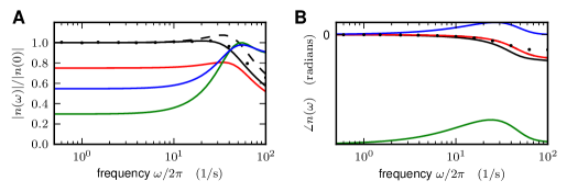
Figure 1: Absolute value (A) and phase (B) of the transfer function for $\mu=18.94\>\mathrm{mV}$, $\sigma=1.5\>\mathrm{mV}$, $\theta=19.5\>\mathrm{mV}$, $V_{r}=14.5\>\mathrm{mV}$, $\tau_{m}=10\>\mathrm{ms}$, $\tau_{s}=1.0\>\mathrm{ms}$. Different contributions $n_{\mathrm{cn}}^{\mathrm{wn}}$ (red), $n_{\mathrm{cn}}^{\mathrm{H}}$ (blue) and $n_{\mathrm{cn}}^{\mathrm{square}}$ (green) and complete solution $\tilde{n}_{\mathrm{cn}}$ (black) compared to white noise case (dashed). Complete transfer functions for white noise and colored noise separately normalized to zero frequency limit $n(0)=\frac{d\nu_{0}}{d\mu}$ and $n_{cn}(0)=\frac{d\nu}{d\mu}$ (cf. Appendix B).

In summary, in these pages we supply intermediate steps of the derivation of the theory presented in (Schuecker et al., 2014) that may prove useful for the reader interested in further developments of the approach. Showing the applicability of the alternative method of reduction of a colored-noise to a white noise system, namely explicitly taking into account the time-dependent boundary condition, may facilitate future extensions of the theory that go beyond the first order in the perturbation parameter $k$. We hope that the pedagogical presentation chosen here, exposing the analogy of the LIF model to the quantum harmonic oscillator and including all intermediate steps of the calculations, will be of use especially for students entering the field with a general background in physics, math or equivalent, but unfamiliar with Fokker-Planck theory.

Appendix A Autocorrelation of $z$

Fourier transformation of the second equation in (1) yields

$$\hat{z} = \frac{k}{1+i\omega k^{2}}\xi(\omega),$$

where $\hat{z}$ denotes the Fourier transform of $z$. The power-spectrum then follows as

$$\langle\hat{z}(\omega)\hat{z}(-\omega)\rangle = k^{2}\frac{1}{(1+i\omega k^{2})(1-i\omega k^{2})},$$

where we used $\langle\xi(\omega)\xi(-\omega)\rangle=1$. We perform the back transform using the residue theorem and assume $s^{\prime}>0$ (which allows us closing the contour in the upper complex half plane due to the term $e^{is^{\prime}\omega}$), thus

$$\langle z(s)z(s+s^{\prime})\rangle = \frac{1}{2\pi}\int k^{2}\frac{e^{i\omega s^{\prime}}}{(1+i\omega k^{2})(1-i\omega k^{2})}\,d\omega$$

$$\stackrel{{\scriptstyle\mathbf{\mathrm{\mathrm{\text{$\mathrm{\text{pole }\omega=\frac{i}{k^{2}}}$}}}}}}{{=}} k^{2}\frac{1}{2\pi}2\pi i\frac{(\omega-\frac{i}{k^{2}})e^{-s^{\prime}/k^{2}}}{ik^{2}(\omega-\frac{i}{k^{2}})(1+1)}$$

$$= \frac{e^{-s^{\prime}/k^{2}}}{2}.$$

If $s^{\prime}<0$ we have to close the contour in the lower half plane. Together we get

$$\langle z(s)z(s+s^{\prime})\rangle = \frac{e^{-|s^{\prime}|/k^{2}}}{2}.$$

Appendix B Zero frequency limit

The zero frequency limit of the colored noise transfer function $n_{\mathrm{cn}}(\omega)$ is given by the derivative of the firing rate (53) with respect to $\mu$. For brevity we introduce $\Psi(x)=u^{-2}F=e^{x^{2}/2}\left(\sqrt{\frac{\pi}{2}}(1+\mathrm{erf}(\frac{x}{\sqrt{2}})\right)$ and $S=\left(\int_{x_{R}}^{x_{\theta}}\Psi\,dx\right)$ so that

$$\tau\nu = \tau\nu_{0}-\frac{\alpha k}{\sqrt{2}}\frac{\left.\Psi\right|_{x_{R}}^{x_{\theta}}}{S^{2}}.$$

With $x=\sqrt{2}\frac{V-\mu}{\sigma}$ we have

$$\frac{d\Psi(x)}{d\mu} = -\frac{\sqrt{2}}{\sigma}\sqrt{\frac{\pi}{2}}\left(xe^{x^{2}/2}(1+\mathrm{erf}(\frac{x}{\sqrt{2}}))+\sqrt{\frac{2}{\pi}}\right)$$

and

$$\frac{dS}{d\mu} = (-\frac{\sqrt{2}}{\sigma})(\Psi(x_{\theta})-\Psi(x_{R})),$$

yielding

$$\frac{d\nu}{d\mu} = \frac{d\nu_{0}}{d\mu}-\frac{\alpha k}{\sqrt{2}\tau}\frac{(\Psi^{\prime}(x_{\theta})-\Psi^{\prime}(x_{R}))S^{2}-(-\frac{\sqrt{2}}{\sigma})(\Psi(x_{\theta})-\Psi(x_{R}))2S((\Psi(x_{\theta})-\Psi(x_{R}))}{S^{4}}$$

$$= \frac{d\nu_{0}}{d\mu}-\frac{\alpha k}{\sqrt{2}\tau}\frac{(\Psi^{\prime}(x_{\theta})-\Psi^{\prime}(x_{R}))S+\frac{2\sqrt{2}}{\sigma}(\Psi(x_{\theta})-\Psi(x_{R}))^{2}}{S^{3}}.$$

Appendix C High frequency limit

For completeness we rederive the high frequency limit of the transfer function in the two-dimensional Fokker-Planck problem, closely following Brunel et al. (2001). The firing rate is given by the probability flux in $y$-direction at threshold, marginalized over $z$. With the ansatz of a sinusoidal modulation of the density we therefore have

$$\nu_{y}(\theta,s) = \int_{-\infty}^{\infty}\frac{1}{k}zP(y_{\theta},z,s)\,dz,$$

$$= \int_{-\infty}^{\infty}\frac{1}{k}z(P(y_{\theta},z)+\hat{P}(y_{\theta},z)e^{i\omega\tau s})\,dz,$$

with (98) resulting in

$$\nu\tau\,n_{\mathrm{cn}}(\omega) = \int_{-\infty}^{\infty}\frac{1}{k}z\hat{P}(y_{\theta},z)\,dz.$$ (110)

Inserting $f(y,s)=-y+\frac{\epsilon\mu}{\sigma}e^{i\omega\tau s}$ in (18) and using the perturbation ansatz $P(y_{\theta},z,s)=P(y_{\theta},z)+\hat{P}(y_{\theta},z)e^{i\omega\tau s}$ we get for $\omega\rightarrow\infty$

$$\hat{P}(y_{\theta},z) = -\epsilon k\frac{\mu}{\sigma}\partial_{z}P(y_{\theta},z),$$ (111)

which shows that the density is necessarily time-modulated up to arbitrary high frequencies. Together with (110) we have

$$\tau\nu\,n_{\mathrm{cn}}(\omega) = -\int_{-\infty}^{\infty}\epsilon\frac{1}{k}zk\frac{\mu}{\sigma}\partial_{z}P(y_{\theta},z)\,dz$$ (112)

$$\stackrel{{\scriptstyle\text{\text{perturbation series in k}}}}{{=}} -\int_{-\infty}^{\infty}\epsilon z\frac{\mu}{\sigma}\partial_{z}\left(Q^{(0)}(y_{\theta})+kQ^{(1)}(y_{\theta},z)\right)\frac{e^{-z^{2}}}{\sqrt{\pi}}\,dz$$

$$\stackrel{{\scriptstyle Q^{(0)}(y_{\theta})=0}}{{=}} -\int_{-\infty}^{\infty}\epsilon z\frac{\mu}{\sigma}k\partial_{z}\left(Q^{(1)}(y_{\theta},z)\frac{e^{-z^{2}}}{\sqrt{\pi}}\right)\,dz$$

$$\stackrel{{\scriptstyle\text{\text{integration by parts}}}}{{=}} \int_{-\infty}^{\infty}\epsilon\frac{\mu}{\sigma}kQ^{(1)}(y_{\theta},z)\frac{e^{-z^{2}}}{\sqrt{\pi}}\,dz$$

$$\stackrel{{\scriptstyle\text{ \eqref{eq:bl_solution} and $r=0$}}}{{=}} \int_{-\infty}^{\infty}\epsilon\frac{\mu}{\sigma}k2\tau\nu_{0}\left(\frac{\alpha}{2}+z+\sum_{n=1}^{\infty}b_{n}(z)\right)\frac{e^{-z^{2}}}{\sqrt{\pi}}\,dz\mbox{}$$

$$\stackrel{{\scriptstyle\text{symmetry and }\text{\cite[citet]{\@@bibref{Authors Phrase1YearPhrase2}{Klosek98}{\@@citephrase{(}}{\@@citephrase{)}}}}}}{{=}} \epsilon k\frac{\mu}{\sigma}\tau\nu_{0}(\alpha-\frac{1}{\sqrt{2}}\sum_{n=1}^{\infty}\frac{N(\sqrt{n})}{n!\sqrt{n}}e^{-\frac{n}{2}}n^{\frac{n}{2}})$$

$$\stackrel{{\scriptstyle\text{\text{\cite[citet]{\@@bibref{Authors Phrase1YearPhrase2}{Brunel01_2186}{\@@citephrase{(}}{\@@citephrase{)}}}}}}}{{\simeq}} 1.3238\,\epsilon k\frac{\mu}{\sigma}\tau\nu_{0}.$$

The numerical value in the last expression is taken from (Fourcaud and Brunel, 2002). We divide by the firing rate in the colored-noise case (53) $\nu=\nu_{0}+k\nu_{1}$ and linearize the right hand side in $k$ which gives

$$n_{\mathrm{cn}}(\omega) \simeq \frac{1.3238\,\epsilon k\mu}{\sigma}\,\frac{\nu_{0}}{\nu_{0}+k\nu_{1}}$$ (113)

$$= \frac{1.3238\,\epsilon k\mu}{\sigma}(1-k\frac{\nu_{1}}{\nu_{0}})+O(k^{2})$$

$$= 1.3238\,\frac{\epsilon k\mu}{\sigma}+O(k^{2}).$$

References

- Schuecker et al. (2014) J. Schuecker, M. Diesmann, and M. Helias, arXiv pp. 1411.0432v7 [cond–mat.stat–mech] (2014).
- Brunel and Hakim (1999) N. Brunel and V. Hakim, Neural Comput. 11, 1621 (1999).
- Lindner and Schimansky-Geier (2001) B. Lindner and L. Schimansky-Geier, Phys. Rev. Lett. 86, 2934 (2001).
- Risken (1996) H. Risken, The Fokker-Planck Equation (Springer Verlag Berlin Heidelberg, 1996).
- Sancho et al. (1982) J. M. Sancho, M. S. Miguel, S. L. Katz, and J. D. Gunton, Phys. Rev. A 26, 1589 (1982).
- Lindenberg and West (1983) K. Lindenberg and B. J. West, Physica A 119, 485 (1983).
- Hanggi et al. (1985) P. Hanggi, T. J. Mroczkowski, F. Moss, and P. V. E. McClintock, Phys. Rev. A 32, 695 (1985).
- Fox (1986) R. F. Fox, Phys. Rev. A 33, 467 (1986).
- Grigolini (1986) P. Grigolini, Phys. Lett. 119, 157 (1986).
- Kłosek and Hagan (1998) M. M. Kłosek and P. S. Hagan, J. Math. Phys. 39, 931 (1998).
- Doering et al. (1987) C. R. Doering, P. S. Hagan, and C. D. Levermore, Phys. Rev. Lett. 59, 2129 (1987).
- Fourcaud and Brunel (2002) N. Fourcaud and N. Brunel, Neural Comput. 14, 2057 (2002).
- Brunel (2000) N. Brunel, J. Comput. Neurosci. 8, 183 (2000).
- Siegert (1951) A. J. Siegert, Phys. Rev. 81, 617 (1951).
- (15) NIST Digital Library of Mathematical Functions, http://dlmf.nist.gov/, Release 1.0.5 of 2012-10-01, online companion to Olver et al. (2010), URL http://dlmf.nist.gov/.
- Abramowitz and Stegun (1974) M. Abramowitz and I. A. Stegun, Handbook of Mathematical Functions: with Formulas, Graphs, and Mathematical Tables (Dover Publications, New York, 1974).
- Brunel et al. (2001) N. Brunel, F. S. Chance, N. Fourcaud, and L. F. Abbott, Phys. Rev. Lett. 86, 2186 (2001).
- Gewaltig and Diesmann (2007) M.-O. Gewaltig and M. Diesmann, Scholarpedia 2, 1430 (2007).
- Olver et al. (2010) F. W. J. Olver, D. W. Lozier, R. F. Boisvert, and C. W. Clark, eds., NIST Handbook of Mathematical Functions (Cambridge University Press, New York, NY, 2010).