The lattice gradient flow at tree level

Abstract:

The cut-off effects of the lattice gradient flow – often called Wilson flow – are calculated on a periodic 4-torus at leading order in the gauge coupling. A large class of discretizations is considered which includes all frequently used cases in practice. It is shown how the results lead to a smoother continuum extrapolation for the $\beta$-function of $SU(3)$ gauge theory with $N_{f}=4$ flavors of fermions.

1 Introduction

It is well established these days that the Yang-Mills gradient flow, or its lattice implementation the Wilson flow [3, 4, 5, 6], is a very useful tool in the non-perturbative study of non-abelian gauge theories. Lattice regularization introduces cut-off dependence which ultimately must be removed to produce continuum results, e.g. [7].

As shown for other observables in QCD, for example quark number susceptibilities, tree-level improvement can lead to a smoother continuum extrapolation than working directly with the original, unimproved quantities. The first systematic investigation of tree-level improvement of the observable $E(t)$ (see section 2 for our definitions) was given in [8] for a large class of discretizations. The necessary leading order lattice perturbation theory calculations were performed in two setups. First, on a periodic 4-torus of finite volume the necessary formulae are given which include all orders in $a^{2}/t$. These may be numerically evaluated to arbitrary precision and can then be used to tree-level improve data from simulations. Second, the infinite volume limit is taken and the results are expanded in $a^{2}/t$ leading to optimal simulation parameters. The latter analytical calculation is checked against the former numerical evaluation. In this contribution we briefly review the results of the infinite volume expansion to order $O(a^{8})$ and the finite volume results valid to all orders in $a^{2}/t$.

Section 2 summarizes the necessary details of the gradient flow, section 3 contains the finite volume discussion including the gauge zero mode, in section 4 the infinite volume limit is taken and the results of the expansion in the lattice spacing are reviewed. We end in section 5 with a number of conclusions and future directions.

2 Gradient flow

The Yang-Mills gradient flow [3, 4, 5] is an evolution in the space of gauge fields given by the gradient of the pure gauge action $S_{\rm YM}$,

$$\frac{dA_{\mu}(t)}{dt}=-\frac{\delta S_{\rm YM}}{\delta A_{\mu}}\;,$$ (1)

where $t$ is the flow time. In a quantum field theory setup this construction can be thought of as defining a complicated observable in the sense that the path integral is over the initial conditions at $t=0$ while the observables are evaluated at $t>0$. Clearly, the gauge field at $t>0$ is a non-linear complicated function of the initial condition at $t=0$. As shown in [3, 4, 5] the flow is essentially a smoothing operation over the range of $\sqrt{8t}$ and leads to $UV$-finite composite operators in some cases where the original composite operator was $UV$-divergent. For example the composite operator $E=-\frac{1}{2}{\rm Tr}F_{\mu\nu}F_{\mu\nu}$ at $t>0$ is finite in perturbation theory provided the gauge coupling is renormalized in the usual way, for example in $\overline{\rm MS\kern-0.5pt}\kern 0.5pt$,

$$\langle t^{2}E(t)\rangle=\frac{3(N^{2}-1)g^{2}}{128\pi^{2}}\left(1+O(g^{2})\right)\;.$$ (2)

The above relation can be turned around and the quantity $E(t)$ can be used to define a renormalized coupling scheme. The scale of the running in infinite volume is $\mu=1/\sqrt{8t}$. The size of cut-off effects in this setup is detailed in section 4.

The calculation of the running coupling on the lattice can most conveniently be performed by step scaling [9] where the running scale is the inverse of the linear size of the system $\mu=1/L$. Using the gradient flow in a step scaling study necessitates that the new scale $t$ is tied to the size of the box and $\sqrt{8t}/L$ is kept constant. Otherwise the problem would have two independent scales, $\sqrt{8t}$ and $L$. This is very similar to using Wilson loops for the definition of the running coupling where the ratio of the size of the Wilson loop and $L$ is kept constant.

The fact that finite volume is involved necessitates to rederive the key equation (2) in finite volume with a given choice of boundary conditions. In [10, 11] periodic boundary conditions were chosen for the gauge field, which we also use here. To leading order the corresponding result is

$$\langle t^{2}E(t)\rangle=\frac{3(N^{2}-1)g^{2}}{128\pi^{2}}\left(1+\delta\left(\sqrt{8t}/L\right)\right)\;,$$ (3)

where

$$\delta(\sqrt{8t}/L) = -\frac{64t^{2}\pi^{2}}{3L^{4}}+\vartheta^{4}\left(\exp\left(-\frac{L^{2}}{8t}\right)\right)-1\;,$$ (4)

using the $3^{rd}$ Jacobi elliptic function $\vartheta$. In section 3 the cut-off effects associated with the finite volume setup are given, i.e. the lattice spacing dependence of the finite volume correction factor $\delta(\sqrt{8t}/L)$ which we will label $\delta(\sqrt{8t}/L,a^{2}/t)$. Note that $\sqrt{8t}/L$ is always kept constant.

In leading order lattice perturbation theory the discretization of $E(t)$ is entirely given by the quadratic term of the lattice gauge action. The gauge action actually enters the calculation in three instances: the action used along the gradient flow, the dynamical gauge action used for the simulation and finally the discretization of the observable $E$ itself. In the continuum all three are the same, $-\frac{1}{2}{\rm Tr}F_{\mu\nu}F_{\mu\nu}$, but on the lattice they may be different. In this work we consider a broad class of discretizations where the first two instances may be the Symanzik improved actions and for the third instance we also consider the symmetric clover discretization along with the Symanzik-improved action. The Symanzik-improved actions may potentially have different improvement coefficients $c_{1}$. Clearly, all cases used in practice are covered by our class of discretizations.

For the frequently used cases, Wilson plaquette ($c_{1}=0$), tree-level Symanzik ($c_{1}=-1/12$) or clover, let us introduce the notation $WWC$, $SSS$, $SSC$, etc, where the order is always Flow-Action-Observable.

3 Finite volume

The quadratic terms in the action that determine the leading order result are well-known. For the Symanzik-improved gauge action with improvement coefficient $c$ we have

$$S_{\mu\nu}=\delta_{\mu\nu}\left({\hat{p}}^{2}-a^{2}c\sum_{\rho}{\hat{p}}_{\rho}^{4}-a^{2}c{\hat{p}}_{\mu}^{2}{\hat{p}}^{2}\right)-{\hat{p}}_{\mu}{\hat{p}}_{\nu}\left(1-a^{2}c({\hat{p}}_{\mu}^{2}+{\hat{p}}_{\nu}^{2})\right)\;,$$ (5)

while for the clover discretization it is [12]

$$K_{\mu\nu}=\left(\delta_{\mu\nu}{\tilde{p}}^{2}-{\tilde{p}}_{\mu}{\tilde{p}}_{\nu}\right)\cos\left(\frac{ap_{\mu}}{2}\right)\cos\left(\frac{ap_{\nu}}{2}\right)\;,$$ (6)

using the lattice momenta

$${\hat{p}}_{\mu}=\frac{2}{a}\sin\left(\frac{ap_{\mu}}{2}\right)\;,\qquad{\tilde{p}}_{\mu}=\frac{1}{a}\sin(ap_{\mu})\;.$$ (7)

In order to have a simple notation let us further introduce

$${\cal S}^{f}_{\mu\nu} = S_{\mu\nu}(c=c_{f})$$

$${\cal S}^{g}_{\mu\nu} = S_{\mu\nu}(c=c_{g})$$ (8)

$${\cal S}^{e}_{\mu\nu} = S_{\mu\nu}(c=c_{e})\;,\qquad{\rm or}\qquad K_{\mu\nu}\;.$$

for the specific choices of the three ingredients: the flow, the dynamical action and the observable. For more details on lattice perturbation theory see [13, 14, 15, 16, 17].

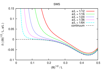
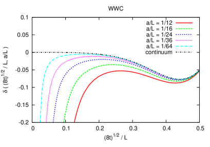
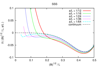
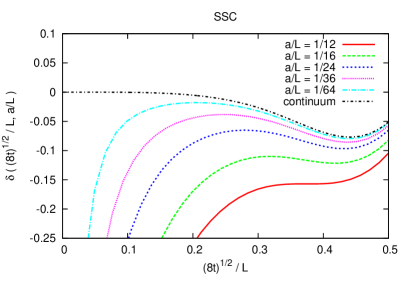
Figure 1: The tree-level finite volume and finite lattice spacing correction factors $\delta(\sqrt{8t}/L,a/L)=C(a^{2}/t,\sqrt{8t}/L)-1$ for four examples, the $SWS$, $WWC$, $SSS$ and $SSC$ cases as a function of $\sqrt{8t}/L$ at various lattice spacings. The continuum result is from [10].

In a periodic finite volume setting special attention needs to be paid to the gauge zero modes. This problem has been dealt with in [10, 11] in the continuum and it is easy to see that to leading order in the coupling the contribution of the zero mode at finite lattice spacing will be the same as in the continuum. The finite volume also means that the momenta are quantized $p_{\mu}=2\pi/L\cdot n_{\mu}$ with integers $n_{\mu}$ and the finite lattice spacing restricts their range to $0\leq n_{\mu}<L/a$. Since the zero mode is treated separately, $n^{2}\neq 0$.

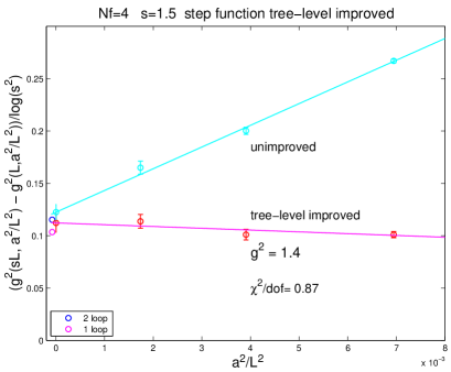
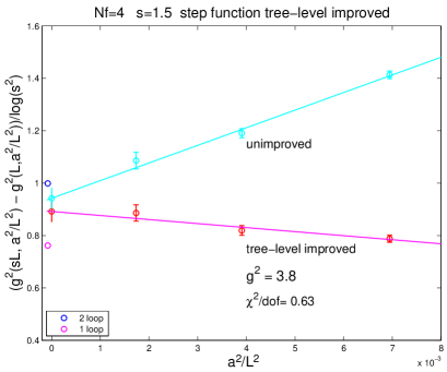
Figure 2: Continuum extrapolations of the discrete $\beta$-function for two selected $g^{2}$ values $1.4$ (left) and $3.8$ (right) for $N_{f}=4$ flavors with and without tree-level improvement. The data is from [10].

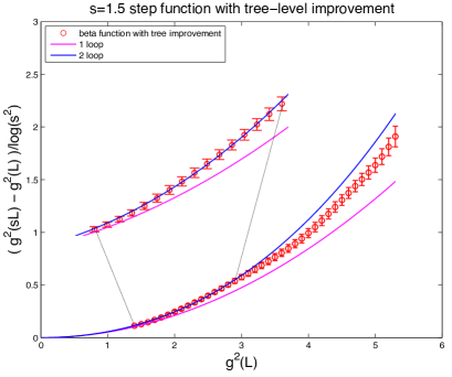
Figure 3: Continuum extrapolated discrete $\beta$-function of $N_{f}=4$ flavors. A section is magnified for better visibility, the data is from [10].

Combining all ingredients the leading order result for $C(a^{2}/t,\sqrt{8t}/L)=1+\delta(\sqrt{8t}/L,a^{2}/t)$ is

$$C(a^{2}/t,\sqrt{8t}/L) = \frac{128\pi^{2}t^{2}}{3L^{4}}+\frac{64\pi^{2}t^{2}}{3L^{4}}\sum_{n_{\mu}=0,\;n^{2}\neq 0}^{L/a-1}{\rm Tr}\,\left(e^{-t\left({\cal S}^{f}+{\cal G}\right)}({\cal S}^{g}+{\cal G})^{-1}e^{-t\left({\cal S}^{f}+{\cal G}\right)}{\cal S}^{e}\right)\;,$$

which may be evaluated numerically to arbitrary precision. Here the exponential terms are coming from the leading order solution of the flow equation (1), the term with the inverse is the leading order gluon propagator and the ${\cal S}^{e}$ term is simply the observable itself. For the sake of convenience a gauge fixing term ${\cal G}_{\mu\nu}={\hat{p}}_{\mu}{\hat{p}}_{\nu}/\alpha$ was introduced. In principle the gauge fixing parameter may be different along the flow and in the propagator but we chose $\alpha=1$ for both. The final result is of course independent of these choices. In front of the sum above is the contribution of the zero mode. The factor $\delta(\sqrt{8t}/L,a^{2}/t)$ is shown in figure 1 for various choices of discretizations and various choices of lattice volume $L/a$. The continuum $\delta(\sqrt{8t}/L)$ factor is also shown for comparison.

In order to test the usefulness of tree-level improvement we consider the $\beta$-function of $SU(3)$ gauge theory with $N_{f}=4$ flavors [10]. The discrete $\beta$-function was computed there and here we reanalyze the data corresponding to two examples of continuum extrapolation, with and without tree-level improvement. The extrapolations for fixed $g^{2}=1.4$ and $g^{2}=3.8$ are shown in figure 2 corresponding to a scale change of $s=3/2$. Clearly the slope of the extrapolation reduced considerably with tree-level improvement. On figure 3 we show the continuum extrapolated discrete $\beta$-function over the entire range of couplings.

4 Infinite volume

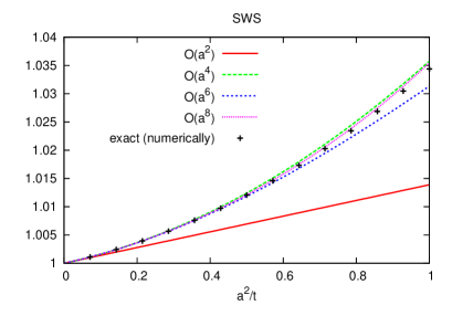
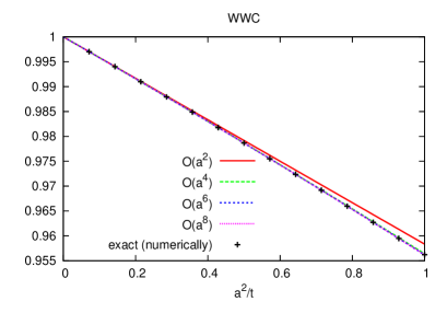
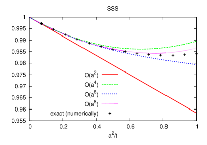
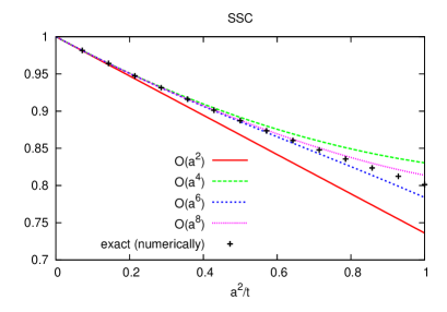
Figure 4: The tree-level improvement factor for four examples, the $SWS$, $WWC$, $SSS$ and $SSC$ cases, starting from only the $O(a^{2})$ correction and including higher and higher order terms. The numerical result containing all orders in $a^{2}/t$, is also shown.

The results in the previous section contained the leading order result in the coupling but all orders in $a^{2}/t$ or equivalently $a^{2}/L^{2}$, in finite volume. In infinite volume one may obtain analytical results if the expressions are expanded in $a^{2}/t$. It is natural to restrict attention to the first few coefficients in an expansion in $a^{2}/t$ because the leading loop effects $g^{2}a^{2}/t$ will certainly be larger than some high power tree-level term $a^{2m}/t^{m}$ for some $m$.

Taking the infinite volume limit of (3) is relatively straightforward. The contribution of the zero modes disappears and the sum turns into a lattice momentum integral,

$$C(a^{2}/t)=\frac{64\pi^{2}t^{2}}{3}\int_{-\frac{\pi}{a}}^{\frac{\pi}{a}}\frac{d^{4}p}{(2\pi)^{4}}{\rm Tr}\,\left(e^{-t\left({\cal S}^{f}+{\cal G}\right)}({\cal S}^{g}+{\cal G})^{-1}e^{-t\left({\cal S}^{f}+{\cal G}\right)}{\cal S}^{e}\right)\;.$$ (10)

The above expression may again be evaluated numerically to arbitrary precision. It may also be expanded in $a^{2}/t$ and the first few coefficients in $C(a^{2}/t)=1+\sum_{m}C_{2m}(a^{2}/t)^{m}$ can be found in [8]. The relative size of the various orders can be judged by looking at figure 4 which shows various truncations and the full, numerically evaluated, result for a few examples.

5 Conclusion

As the application of the gradient flow expands to more areas a systematic understanding of its cut-off effects becomes essential. In this contribution we reviewed the size of cut-off effects for the particularly important observable $E(t)$ for a large class of discretizations at tree-level of the coupling. The main motivation was to understand cut-off effects in setups frequently used in practice. A natural next step would be to obtain the corresponding formulae to 1-loop.

References

- [1]
- [2]
- [3] M. Luscher, Commun. Math. Phys. 293, 899 (2010) [arXiv:0907.5491 [hep-lat]].
- [4] M. Luscher, JHEP 1008, 071 (2010) [arXiv:1006.4518 [hep-lat]].
- [5] M. Luscher, PoS LATTICE 2010, 015 (2010) [arXiv:1009.5877 [hep-lat]].
- [6] M. Luscher and P. Weisz, JHEP 1102, 051 (2011) [arXiv:1101.0963 [hep-th]].
- [7] S. Borsanyi, S. Durr, Z. Fodor, C. Hoelbling, S. D. Katz, S. Krieg, T. Kurth and L. Lellouch et al., JHEP 1209, 010 (2012) [arXiv:1203.4469 [hep-lat]].
- [8] Z. Fodor, K. Holland, J. Kuti, S. Mondal, D. Nogradi and C. H. Wong, JHEP 1409, 018 (2014) [arXiv:1406.0827 [hep-lat]].
- [9] M. Luscher, P. Weisz and U. Wolff, Nucl. Phys. B 359, 221 (1991).
- [10] Z. Fodor, K. Holland, J. Kuti, D. Nogradi and C. H. Wong, JHEP 1211, 007 (2012) [arXiv:1208.1051 [hep-lat]].
- [11] Z. Fodor, K. Holland, J. Kuti, D. Nogradi and C. H. Wong, PoS LATTICE 2012, 050 (2012) [arXiv:1211.3247 [hep-lat]].
- [12] P. Fritzsch and A. Ramos, JHEP 1310, 008 (2013) [arXiv:1301.4388 [hep-lat]].
- [13] P. Weisz, Nucl. Phys. B 212, 1 (1983).
- [14] K. Symanzik, Nucl. Phys. B 226, 187 (1983).
- [15] P. Weisz and R. Wohlert, Nucl. Phys. B 236, 397 (1984) [Erratum-ibid. B 247, 544 (1984)].
- [16] M. Luscher and P. Weisz, Commun. Math. Phys. 97, 59 (1985) [Erratum-ibid. 98, 433 (1985)].
- [17] M. Luscher and P. Weisz, Phys. Lett. B 158, 250 (1985).