Crystal-liquid interfacial free energy of hard spheres via a novel thermodynamic integration scheme

Abstract

The hard sphere crystal-liquid interfacial free energy, ($\gamma_{\rm cl}$), is determined from molecular dynamics simulations using a novel thermodynamic integration (TI) scheme. The advantage of this TI scheme compared to previous methods is to successfully circumvent hysteresis effects due to the movement of the crystal-liquid interface. This is accomplished by the use of extremely short-ranged and impenetrable Gaussian flat walls which prevent the drift of the interface while imposing a negligible free-energy penalty. We find that it is crucial to analyze finite-size effects in order to obtain reliable estimates of $\gamma_{\rm cl}$ in the thermodynamic limit.

I Introduction

Since the discovery of a fluid-to-solid transition in hard spheres by computer simulations alder-wainright57 , the hard sphere model has become one of the paradigms mulerolnp753 for the study of nucleation and crystal growth auerfrenkel2001 ; lairdaminiprl2006 ; zykova2009 ; zykova2010 ; filion2010 . The simplicity of the hard sphere interaction potential allows for the development of theoretical and computational approaches that allow for quantitative predictions in the context of crystallization phenomena curtin89 ; marr94 ; marr95 ; gruhn2001 ; snook2003 ; pusey2009 ; tanaka2010 ; schilling2010 . The crucial thermodynamic parameter which governs the mechanism of homogeneous nucleation and subsequent growth of the crystal from the melt is the crystal-liquid interfacial free energy, $\gamma_{\rm cl}$, defined as the reversible work required to form an unit area of a crystal-liquid interface adamson97 . The homogeneous nucleation rate as well as the final morphology of the resulting crystal are strongly dependent on the magnitude and anisotropy of this quantity turnbull-cech50 ; turnbull50 ; turnbull52 ; woodruff73 ; tiller91 .

Several simulation as well as theoretical approaches [based on Density Functional Theory (DFT)] have attempted to determine the interfacial free energy of hard-sphere systems, though there have been some discrepancy in the results obtained from these various methods davidchack-laird2000 ; cacciuto2003 ; laird-davidchack2005prl ; laird-davidchack2005jpcb ; davmorrislaird2006 ; davidchack2010 ; hartel2012 ; martin2012 . A direct determination of $\gamma_{\rm cl}$ for hard sphere systems was made in Ref. davidchack-laird2000 using a thermodynamic integration straatsma93 ; frenkel-smit02 approach known as the “cleaving wall” method. Later, the estimates for $\gamma_{\rm cl}$ were revised davidchack2010 after fixing an error in the previous TI scheme. The same authors carried out TI simulations with the soft-sphere potential and extrapolated the results to the hard-sphere limit laird-davidchack2005prl ; laird-davidchack2005jpcb . Data in Ref. laird-davidchack2005prl were a little higher than those reported for the pure hard sphere system davidchack2010 . The most reliable estimates from an indirect approach based on capillary fluctuations hartel2012 were about $10\%$ higher than those reported in Ref. davidchack2010 . Results from DFT hartel2012 , while in good agreement with the “cleaving wall” and capillary fluctuation methods as regards the anisotropy is concerned, yielded larger values for the magnitude of $\gamma_{\rm cl}$. Results from the Tethered Monte Carlo approach are consistent with the capillary fluctuation method hartel2012 but are a few percentages higher than those reported in Ref. davidchack2010

In the “cleaving walls” scheme davidchack-laird2000 ; davidchack2010 , the thermodynamic integration was carried out by using an external wall, consisting of particles arranged in an ideal lattice structure, to split the bulk phases and then join them together. Finally, the walls were removed resulting in crystal and liquid phases separated by two interfaces. In this approach, there were uncontrolled hysteresis errors in the last step when the external walls were removed. When both phases are joined together, the interface is formed at the walls. However, when such “cleaving walls” are gradually removed, the interface drifts on account of thermal fluctuations. In long simulations, the interfaces can travel far from the walls by freezing at one end and simultaneously melting at the other end davlaird96 ; davidchack-laird03 ; davidchack2010 . As a result, the reverse process (when the cleaving walls are reinserted) does not retrace the same path as the forward process, showing the existence of hysteresis. This affects the accuracy in the final estimates of $\gamma_{\rm cl}$. While the interfacial drift is not a problem for liquid-liquid interfaces schmitz2014 , it is far more severe for the crystal-liquid interface and needs to be overcome in order to obtain accurate values for $\gamma_{\rm cl}$.

In a recent work, we have developed a novel TI scheme to compute $\gamma_{\rm cl}$ for the Lennard-Jones potential benjamin-horbach2014 . Our method is able to circumvent problems associated with the drift of the crystal-liquid interface and provides a better control of hysteresis errors associated with the latter drift. The strategy was to use extremely short-ranged and flat Gaussian walls to constrain the position of the interface while imposing a negligible free energy penalty. Another novelty of our scheme was the use of structured walls consisting of frozen-in crystalline layers to smoothly transform the system from separate bulk phases to two interfaces in contact with the bulk fluid and crystal phases.

Apart from the TI scheme, the reliability of $\gamma_{\rm cl}$ estimates also depends on properly accounting for the finite-size effects. However, few previous works on the determination of $\gamma_{\rm cl}$ via molecular simulations include a discussion on finite size effects. In a recent work, Schmitz et al. schmitz2014 proposed a scaling relation based on capillary wave theory, to take into account finite size corrections and get accurate values for the interfacial free energies in the thermodynamic limit. In our earlier work benjamin-horbach2014 on the crystal-liquid interfacial free energy for Lennard-Jones systems, we obtained results consistent with their theory.

In this work, we compute $\gamma_{\rm cl}$ for hard spheres using Molecular Dynamics (MD) in combination with TI. We will determine $\gamma_{\rm cl}$ for the (100), (110) and (111) orientations of the face centered cubic crystal-liquid interface. The hard sphere interactions are described by a very short-ranged inverse power-law potential (see below). The reason for using such a short-ranged continuous potential is the easy adaptability of our TI scheme developed for the continuous LJ potential into the soft-sphere potential. Since our TI scheme involves a direct modification of the interaction potential, it is easier to fit it into a conventional MD simulation with continuous potential rather than to a collisional event-driven MD algorithm for a discontinuous hard-sphere potential rapaport04 .

To account for errors due to finite size effects and estimate $\gamma_{\rm cl}$ in the thermodynamic limit, a careful analysis was carried out at several system sizes in the framework of capillary wave theory binder82 ; schmitz2014 . We obtain results consistent with the predictions of capillary wave theory showing that the introduction of the flat wall does not suppress capillary fluctuations. The success of our scheme indicates that our TI approach is also well suited for very short-ranged potentials.

In the next section, we introduce the potential and then describe the TI scheme in Sec. III. The details of the simulation are given in Sec. IV and results are presented in Sec. V. Finally, we end with a conclusion in Sec. VI.

II Interaction Potential

Hard-sphere interactions between a particle $i$ at position $\vec{r}_{i}$ and a particle $j$ at position $\vec{r}_{j}$, separated by a distance $r_{ij}=|\vec{r}_{i}-\vec{r}_{j}|$ are approximated by the inverse power-law potential

$$\phi(r_{ij})=\epsilon\left(\frac{\sigma}{r_{ij}}\right)^{n}\quad\quad{\rm with}\quad\quad n=256,$$ (1)

where $\epsilon$ and $\sigma$ set the energy and length scale, respectively. For computational efficiency, the potential was cut-off at a distance $r_{\rm c}=1.2\,\sigma$, where the potential has a value $10^{-21}\epsilon/k_{\rm B}T$. With the exponent $n=256$, the parameters for solid-fluid coexistence at the temperature $k_{\rm B}T=1.0\,\epsilon$ (with $k_{\rm B}$ the Boltzmann constant) are very close to those for the hard-sphere system zykova2010 , in agreement with recent findings lange2009 (see below).

III Method

The interfacial free energy $\gamma_{\rm cl}$ is the excess free-energy per area that results from the formation of an interface between the crystal and the liquid phase. It can be expressed via the difference between the free energy of the inhomogeneous system with crystal-liquid interface, $F_{\rm cl}$, and the sum of the bulk free energies of the crystal and liquid, $F_{\rm c}$ and $F_{\rm l}$, respectively,

$$\gamma_{\rm cl}=\frac{F_{\rm cl}-(F_{\rm c}+F_{\rm l})}{A}$$ (2)

with $A$ the area of the interface.

Computing $\gamma_{\rm cl}$ via thermodynamic integration involves joining together bulk crystal and liquid phases at coexistence to form an inhomogeneous system involving the individual phases separated by two interfaces. To ensure a path with minimal hysteresis, the crystal phase should be perturbed as little as possible such that no stress is generated in the crystal when it comes into contact with the liquid phase.

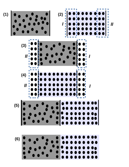
Figure 1: Schematic of the TI scheme adopted in this work. Particles in the light and dark simulation boxes represent the crystal and the liquid phases, respectively. For details see text.

Here, we provide a novel TI scheme to compute $\gamma_{\rm cl}$ for the inverse power potential, Eq. (1). Our TI scheme is based on an earlier approach used to obtain the crystal-liquid interfacial free energy for a Lennard-Jones potential benjamin-horbach2014 . Compared to previous TI methods such as the “cleaving potential” broughton-gilmer86 or “cleaving walls” davidchack-laird2000 ; davidchack-laird03 ; laird-davidchack2005prl ; laird-davidchack2005jpcb ; davidchack2010 scheme, our approach differs in two crucial ways. Firstly, in order to achieve minimal perturbation of the crystalline phase during the transformation, the liquid should be ordered into a crystal-like layers near the boundaries of the simulation box and this ordering must be compatible with the actual structure of the crystal phase. In our TI scheme, this is achieved by introducing a structured solid wall, consisting of particles belonging to the crystal phase, frozen into their instantaneous equilibrium position. Interactions between the particles in the bulk phases and the structured wall are of the same kind as that between the bulk particles.

Secondly, to tackle the problem associated with the movement of the crystal-fluid interface due to thermal fluctuations davlaird96 , a Gaussian flat wall is introduced to prevent the interface from drifting during the simulation. However, unlike the previous TI scheme benjamin-horbach2014 , where an extremely short-ranged flat wall is introduced at the beginning of the scheme, here in the first step we introduce a flat wall with a similar range as the interaction potential between the particles. Only in the final step, the range of this wall is gradually reduced to a value much smaller than the effective size of the particles $\sigma$ (about $10^{4}$ times less). This trick saves computational time as a short-time step needs to be used in the final step to integrate the short-ranged forces. The use of a multiple time-step algorithm frenkel-smit02 in the final step further improves the computational efficiency of the scheme.

Initially, bulk liquid and crystal phases are simulated in a box with dimensions $L_{\rm x}\times L_{\rm y}\times L_{\rm z}$ such that the two phases have the same volume but different particle numbers. The final state consists of two crystal-liquid interfaces connecting the bulk phases, with a total length $2L_{\rm z}$ along the $z$ direction. The TI scheme proceeds via six steps and in each step the transformations are carried out by directly modifying the interaction potential by a parameter $\lambda$. This idea is similar to the TI scheme presented in earlier works to compute $\gamma_{\rm cl}$ and the interfacial free energies of liquid and crystal phases in contact with flat and structured walls benjamin-horbach2012 ; benjamin-horbach2013 ; benjamin-horbach2014 . The specific choices of the $\lambda$ parameterizations adopted below, yielded smooth thermodynamic integrands allowing for an accurate numerical calculation of the integrals. In the following, we outline the TI scheme, in detail.

Steps 1 and 2: The initial thermodynamic state of our system consists of separate bulk liquid and crystal phases with periodic boundary conditions (along the $z$ direction), while the final state involves liquid and crystal separated by two interfaces. To reach the final state, at some point during the transformation, interactions between the two sides of each phase through the periodic boundaries must be switched off while the interactions between the two phases must be turned on. While rearranging the periodic boundaries, it must be ensured that the particles belonging to each phase remain inside their respective simulation cells and do not cross the boundaries such that density of each phase in its box remains at the respective coexistence density. For this purpose, in the first and second steps, a Gaussian flat wall is gradually introduced at both ends of the liquid and crystal simulation boxes respectively, along the $z$ direction [sketch (1) in Fig. 1]. The periodic boundary conditions are kept intact. This wall acts as a barrier to prevent the liquid and crystal particles from crossing the boundaries. The transformation is carried out by gradually increasing the height of the potential barrier.

The interaction of a particle $i$ with the flat wall is modeled by a Gaussian potential,

$$u_{\text{fw}}(z_{iw})=a\exp\left[-\left(\frac{z_{iw}}{b}\right)^{2}\right]\,,$$ (3)

with $z_{iw}$ the distance of the particle from the wall in $z$-direction. The height and range of the Gaussian potential is determined by the variables $a$ and $b$. At a temperature $T=1.0$, we chose $a=25k_{\rm B}T/\epsilon$, such that the particles cannot overcome the barrier. $b$ was set to $0.027\,\sigma$. For this value of $b$, the bulk density does not change in the presence of the wall.

The parameter $\lambda$ is coupled to the flat wall as follows,

$$\begin{split}u_{\text{fw}}(\lambda,z_{iw})=&\lambda^{2}u_{\text{fw}}(z_{iw})\end{split}$$ (4)

At $\lambda=0$, there is no wall and as $\lambda$ increases the wall becomes more and more impenetrable.

The $\lambda-$dependent Hamiltonian for steps 1 and 2 takes the form

$$\begin{split}H_{1(2)}(\lambda)=\sum_{i=1}^{N}\frac{{{\bf p}_{i}^{2}}}{2m}+{U_{\text{pp}}^{\text{l(c)}}}+\lambda^{2}{U_{\text{fw}}^{\text{l(c)}}}\,,\end{split}$$ (5)

where, $H_{\rm 1(2)}$ represents the Hamiltonian for interaction of the flat wall with the liquid (crystal) and ${\bf p}_{i}$ and $m$ denote the momentum and mass of particle $i$ with all particles having the same mass. The potential energy due to particle-particle interactions is represented by ${U_{\text{pp}}^{\text{l(c)}}}=\sum_{i=1}^{N^{\text{l(c)}}}\sum_{j=i+1}^{N^{\text{l(c)}}}u(r_{ij})$. The interaction potential of particles with the flat wall is denoted by ${U_{\text{fw}}^{\text{l(c)}}}=\sum_{i=1}^{N^{\text{l(c)}}}u_{\text{fw}}(z_{\text{iw}})$, where the superscript l(c) refers to particles in liquid (crystal) phase and $N^{\text{l(c)}}$ is the total number of liquid (crystal) particles.

Steps 3 and 4: From the two sides of the crystal simulation cell, containing $1-2$ layers of crystalline particles frozen into an instantaneous equilibrium configuration, two structured walls were constructed. As shown in Fig. 1, these walls are juxtaposed at the appropriate ends of the liquid and crystal simulation cells corresponding to steps 3 and 4, respectively. The flat walls are still present to prevent particles from crossing the boundaries. During the transformation, the structured walls are gradually switched on, while interactions through the periodic boundaries along the $z$ direction are gradually switched off.

The $\lambda$-dependent Hamiltonian for step 3 is given by,

$$\begin{split}H_{3}(\lambda)=\sum_{\text{i=1}}^{N}\frac{{\bf p}_{i}^{2}}{2m}+{{U}_{\text{pp}}^{\text{l}}}+(1-\lambda)^{256}{{U^{\ast}}_{\text{pp}}^{\text{l}}}\\ +\lambda^{256}{U_{\text{pw}}^{\text{l}}}+{U_{\text{fw}}^{\text{l}}}\end{split}$$ (6)

Since the inverse-power potential (Eq. 1) is very short-ranged, and the liquid particles being present close to the boundaries of the simulation box at the beginning of this step, a rapidly decaying $\lambda$-function for the periodic boundaries ensures a smoothly varying thermodynamic integrand. Effectively, this transformation is carried out by gradually modifying the size of the particles, i.e. $\epsilon([(1-\lambda)\sigma]/r)^{256}$ and $\epsilon([\lambda\sigma]/r)^{256}$ for switching off the periodic boundaries and switching on the structured walls, respectively.

In the “cleaving walls” TI scheme, the interaction between the individual phases and the walls was brought about by moving the walls towards the bulk liquid and crystal phases. This required the use of a complex “corrugated cleaving plane” davidchack-laird03 ; davidchack2010 , which is compatible with the structure of the wall. However, in our TI scheme, the interaction between the two phases or between each individual phase and the structured walls takes place across a flat plane. As shown above, this is achieved by directly modifying the interaction potentials to carry out the transformations, leading to a simple and straightforward algorithm.

The corresponding Hamiltonian for step 4 is given by,

$$\begin{split}H_{4}(\lambda)=\sum_{\text{i=1}}^{N}\frac{{\bf p}_{i}^{2}}{2m}+{{U}_{\text{pp}}^{\text{c}}}+(1-\lambda)^{8}{{U^{\ast}}_{\text{pp}}^{\text{c}}}\\ +\lambda^{256}{U_{\text{pw}}^{\text{c}}}+{U_{\text{fw}}^{\text{c}}}\end{split}$$ (7)

Since it is necessary to maintain the crystalline structure throughout the transformation, in Eq. (7), the periodic boundaries are switched off gradually such that these interactions become weaker only when the structured walls are already strongly interacting with the crystal phase.

In Eqs. (6) and (7), ${{U^{\ast}}_{\text{pp}}^{\text{c(l)}}}$ specifies the periodic boundary interactions, while ${U_{\text{pp}}^{\text{c(l)}}}$ corresponds to the bulk interactions. Interactions between the individual phases and the structured wall particles is denoted by $U_{\text{pw}}$, where ${U_{\text{pw}}^{\text{c(l)}}}=\sum_{i=1}^{N^{\text{c(l)}}}\sum_{j=1}^{N^{\text{w}}}u_{\text{pw}}(r_{{ij}})$, with $N^{\text{w}}$ being the total number of particles in the structured walls. The same inverse power potential was used for $u_{\text{pw}}$, as given by Eq. (1), with the parameter $\epsilon$ replaced by $\epsilon_{\rm pw}$. Throughout the transformation in steps 3 and 4 as well as in subsequent steps, $\epsilon_{\rm pw}/\epsilon=1$ was kept constant, where $\epsilon$ refers to the interaction strength between the particles of the system.

Step 5: In this step, the individual liquid and crystal phases are gradually brought together in the presence of the Gaussian flat walls, while the structured walls are removed. Since the periodic boundary conditions in the two phases are already switched off, only interactions between the two phases need to be turned on [see (5) in Fig. 1]. At the end of this step, the resulting thermodynamic state consists of bulk crystal and liquid phases separated by two interfaces whose position is tied to the position of the flat walls.

The Hamiltonian corresponding to step 5 is

$$\begin{split}H_{5}(\lambda)=\sum_{\text{i=1}}^{N_{p}}\frac{{\bf p}_{\text{i}}^{2}}{2m_{i}}+{{{U}_{\text{pp}}^{\text{c(l)}}}}+\lambda^{2}\left(\frac{1+\lambda}{2}\right)^{\rm 256}{U_{\text{pp}}^{\text{c+l}}}\\ +(1-\lambda)^{2}(1-\lambda/2)^{256}{U_{\text{pw}}^{\text{c(l)}}}+{U_{\text{fw}}^{\text{c(l)}}},\end{split}$$ (8)

where the interaction potential between the liquid and crystal phases is denoted by, ${U_{\text{pp}}^{c+l}}=\sum_{i=1}^{N^{\text{l}}}\sum_{j=1}^{N^{\text{c}}}u(r_{{ij}})$. In Eq. (8), there is a one-to-one correspondence in the $\lambda$-parameterizations such that interactions between the crystal and liquid phases are turned on while interactions with the structured wall are switched off to ensure a smoothly varying thermodynamic integrand.

Step 6: The last step involves removing the flat walls and it is difficult to achieve total control over the reversibility of the scheme. Due to thermal fluctuations, the two interfaces can move by melting on one side and refreezing on the other side, if the potential barrier due to the walls is weak enough, i.e. ($a\leq k_{\rm B}T$). However, this makes the transformation irreversible since if the walls are reinserted, the position of the interfaces will not coincide with the position of the walls. As a result, in the two simulation boxes a mixture of liquid and crystal phases will be obtained and one cannot retrace the previous steps in the reverse direction to reach the initial state consisting of independent liquid and crystal phases at their respective coexistence densities.

However, by a clever scheme one can reduce the error due to the resulting hysteresis in the TI path to a negligible value such that it does not affect the accuracy in the final estimates of $\gamma_{\rm cl}$. This is achieved by breaking step 6 into two sub-steps 6a and 6b. In the first sub-step, the range of the Gaussian flat wall is gradually reduced while maintaining the same height for the potential barrier. In principle, this sub-step is reversible since, the particles still cannot cross the flat wall barrier at the end of this step. In the next step, 6b, the height of the barrier is slowly switched off such that in the end one has the desired state consisting of liquid and crystalline phases separated by two interfaces. This transformation is no more reversible due to the movement of the interface. However, if the range of the Gaussian flat wall has been reduced significantly in step 6a such that very few particles interact with the wall, the contribution of step 6b would be negligible in comparison to the magnitude of $\gamma_{\rm cl}$ and can be ignored.

The Hamiltonian corresponding to sub-step 6a is given by

$$\begin{split}H_{6a}(\lambda)=\sum_{i=1}^{N}\frac{{{\bf p}_{i}^{2}}}{2m}+{U_{\text{pp}}^{\text{l(c)}}}+{U_{\text{fw}}^{\text{l(c)}}}(\lambda)\,,\end{split}$$ (9)

with

$$\begin{split}u_{\text{fw}}(z_{iw},\lambda)=&a\exp(-[z_{iw}/b(\lambda)]^{2})\,.\end{split}$$ (10)

where ${U_{\text{fw}}^{\text{l(c)}}}(\lambda)=\sum_{i=1}^{N_{\rm l(c)}}u_{\text{fw}}(z_{iw},\lambda)$. In Eq. (10), $b(\lambda)={(1-\lambda)}^{2}b^{\prime}$ with $b^{\prime}=0.027\sigma$ and $\lambda$ varies from $0$ to $0.893$ such that the parameter $b(\lambda)$ is reduced from $0.027\sigma$ to $0.0003\sigma$.

In the next sub-step, 6b, the extremely short-ranged Gaussian walls are gradually switched off. The Hamiltonian for this sub-step is

$$\begin{split}H_{6b}(\lambda)=\sum_{i=1}^{N}\frac{{{\bf p}_{i}^{2}}}{2m}+{U_{\text{pp}}^{\text{l(c)}}}+{(1-\lambda)^{2}}{U_{\text{fw}}^{\text{l(c)}}}\,,\end{split}$$ (11)

In this last step, $b$ was kept at the same value as at the end of step 6a, viz. $b=0.0003\sigma$. In principle, the flat wall could be made even more short-ranged by varying $\lambda$ in step 6a up to, say $0.99$. However, our simulations showed that reducing the range of the flat wall to such a low value is unnecessary for our purpose, since the combined numerical and statistical errors from steps one to five would be much larger than the total contribution from step 6b.

Generally, the contribution of step 6b, depends on the average density of particles in the interface region. Prior work on the crystal-liquid interface corresponding to hard sphere systems has shown that density near the interface is the mean of the bulk liquid and solid coexistence densities davlaird96 . Even accounting for capillary fluctuations, the average density will not be very far from this mean value. Therefore, the contribution of step 6b will be close to that obtained for the flat wall-liquid interface. For example, at $b=0.0003\sigma$, the excess free-energy of the fluid in contact with the flat-wall was about $10$ times less than the statistical errors from steps 1-6a. For the crystal, the excess free energy was about $1000$ time less than the typical statistical errors. Since our simulations yield such a small free energy difference for liquid in contact with the flat wall at $b=0.0003\sigma$, it is clear that step 6b will yield a similar negligible value and hence this step can effectively be ignored. In general, our simulations indicate a negligible value (less than $10^{-4}k_{\rm B}T$) for the liquid-flat wall free energy difference and hence that of step 6b, as well, if $b\sim 10^{-4}\sigma$.

We carried out several independent runs for one system size, both in the forward as well as reverse directions to check the reversibility of step 6b and obtained the free-energy difference from runs which yielded the least hysteresis davidchack2010 ; davidchack-laird03 . Our simulation results showed a negligible contribution for this step of the order of $0.00005$ $k_{\rm B}T$ for the (100) and (111) orientations and of the order $0.0005k_{\rm B}T$ for the (110) orientation. Since, the combined statistical and numerical errors in the previous steps (1-6a) are in the range $0.003-0.005k_{\rm B}T$, this last step was not performed for other system sizes at which simulations were carried out.

The free energy difference in the various steps can be computed as

$$\Delta F_{\rm i}=\int_{0}^{1}\left\langle\frac{\partial H_{\rm i}}{\partial\lambda}\right\rangle d\lambda$$ (12)

where $i$ varies from $1$ to $6$ corresponding to the six steps.

The interfacial free energy $\gamma_{\rm cl}$ is obtained by adding the the free energy differences corresponding to the six steps, divided by the total interfacial area $A$,

$$\gamma_{\rm cl}=\frac{\sum_{i=1}^{6}{\Delta F}_{\rm i}}{A}\,,$$ (13)

with $A=2L_{\rm x}L_{\rm y}$ (the factor 2 takes into account the presence two independent planar crystal-liquid interfaces, cf. Fig. 1).

IV Simulation Details

Molecular Dynamics (MD) simulations were carried out in the canonical ensemble with the total number of particles $N=N_{\rm l}+N_{\rm c}$, volume $V$ and temperature $T$ maintained constant. Constant temperature was achieved by assigning every 200 time steps random velocities to the particles distributed according to the Maxwell-Boltzmann distribution. Newton’s equations of motion were integrated according to the velocity Verlet algorithm allen-tildesley87 . During steps one to five of our TI scheme, a time-step $\Delta t_{\rm large}=0.0005\tau$ (with $\tau=\sqrt{(m{\sigma}^{2}/\epsilon)}$) was used. In the sixth step, to take into account the extremely short-range forces due to the Gaussian flat wall, a multiple time-step scheme frenkel-smit02 was applied, where in combination with $\Delta t_{\rm large}$, a smaller time-step of $\Delta t_{\rm small}=0.000025\,\tau$ was used. It was observed that this slowed down the simulations by approximately a factor of two.

The coexistence densities for the inverse-power potential, Eq. 1, as computed using the free-solidification method zykova2010 ; kuhn13 , at the temperature $T=1.0$, are $\rho_{\rm l}^{\rm inv}=0.933\,\sigma^{-3}$ for the liquid phase and $\rho_{\rm c}^{\rm inv}=1.030\,\sigma^{-3}$ for the crystal phase; the coexistence pressure is given by $P_{\rm co}^{\rm inv}=11.46k_{\rm B}T/{\sigma}^{3}$ undulating_subst_2014 . In comparison, the coexistence parameters of the actual hard-sphere system are $\rho_{\rm l}^{\rm HS}=0.940{\sigma}^{-3}$, $\rho_{\rm c}^{\rm HS}=1.041{\sigma}^{-3}$ and $P_{\rm co}^{\rm HS}=11.576k_{\rm B}T/{\sigma}^{3}$ zykova2010 .

From these co-existence values one can define an effective dimensionless diameter $\sigma^{\rm eff}=\sigma(\rho_{\rm c}^{\rm HS}/\rho_{\rm c}^{\rm inv})^{-1/3}$, which can be used as a scaling parameter to compare the two systems. Such an effective diameter can also be obtained using the co-existence pressure value as well as the coexistence density of the liquid. It is observed that using the crystal co-existence density and the co-existence pressure as the scaling variable leads to the same effective diameter, viz. $\sigma^{\rm eff}=1.0035\sigma$, while use of the liquid co-existence density leads to a slightly lower effective diameter $\sigma^{\rm eff}=1.0024\sigma$. We will use the effective diameter value $\sigma^{\rm eff}=1.0035\sigma$ to compare the crystal-liquid interfacial free energy obtained for the inverse power-law model with the hard-sphere values. The equivalent values for the hard-sphere model are obtained as $\gamma_{\rm cl}^{\rm HS}=\gamma_{\rm cl}^{\rm inv}{{\sigma^{\rm eff}}^{2}}/{k_{\rm B}T}$, where $\gamma_{\rm cl}^{\rm inv}$ is the interfacial free energy corresponding to the inverse power-law potential.

We obtain $\gamma_{\rm cl}$ for the (100), (110) and (111) orientations of the face-centered cubic crystal with respect to the liquid at the interface. To study finite-size effects, simulations were carried out at various system sizes for the (100) orientation of the interface, ranging from around $7000$ to $34000$ particles, with various lateral dimensions and with a total longitudinal dimension of about $80\sigma$. For the other two orientations, simulations were carried out only at the largest system sizes. The dimensions of our system along with the total number of particles are specified in Table I.

To generate initial configurations, liquid and crystal phases were equilibrated for about $2\times 10^{6}$ time steps (in steps of ${\Delta t}_{\rm large}$) at their respective co-existence densities. Both phases were simulated in cells of identical dimensions with $N_{\rm l}<N_{\rm c}$, since $\rho_{\rm l}<\rho_{\rm c}$. To calculate $\gamma_{\rm cl}$ via TI, independent runs were carried out at $50-100$ values equally spaced intervals of $\lambda$ between the initial and final states in order to obtain smooth thermodynamic integrands. At every value of $\lambda$, the system was first equilibrated at $\lambda=0$ for $10^{4}$ time steps and then $\lambda$ was continuously increased until the desired value of $\lambda$ was reached. The number of time steps to carry out this switch varied from $2.5\times 10^{5}$ to $10^{6}$ time steps for the various TI steps. After the final value $\lambda_{i}$ was reached, the system was further equilibrated for times varying from $10^{6}$ to $4\times 10^{6}$ time steps. Then the production runs were carried out over a period varying from $10^{6}$ to $5\times 10^{6}$ time-steps for the different TI steps to obtain the desired statistical accuracy.

For steps 3, 4 and 5, a cubic spline interpolation of the bare data was performed to obtain the thermodynamic integrand at 100 intervals between $\lambda=0$ and $\lambda=1$. Then, Simpson’s rule was used to numerically calculate the integral. For steps 1, 2 and 6, the thermodynamic integrals were calculated numerically using the trapezoidal rule from the bare data. Statistical errors were calculated by partitioning the production runs into $5$ blocks and then determining the standard deviation from these $5$ samples.

To check the reversibility of each step in the TI scheme both simulations were also carried out in the reverse direction, to detect any hysteresis in the transformation. The initial state for the reverse TI simulations corresponded to the final state of the forward TI path. The final values for $\gamma_{\rm cl}$ reported in Table I correspond to an average of the free energy differences obtained from the forward and reverse TI simulations.

V Results

The thermodynamic integrands for the various steps are plotted in Figs.2 to 5, for the (100) orientation of the crystal-liquid interface. The data corresponds to the largest system size of $32205$ particles with dimensions $20.43\times 20.43\times 78.58$ (in units of $\sigma^{-3}$). Figure 2 shows the thermodynamic integrand corresponding to steps 1 and 2 of our scheme. It is clear that the area under the thermodynamic integrand curve corresponding to the crystal is negligible as compared to the liquid. Since the crystal is positioned symmetrically with respect to the two ends of the simulation cell, the location of the flat walls (at $z=0$ and $L_{\rm z}$) coincides with a density minimum between two crystalline layers. Moreover, the crystal has a small diffusivity as compared to the liquid. Therefore, the free energy cost of inserting a flat wall in the crystal is negligible compared to that in the liquid.

For the (100), (110) and (111) orientations of the crystal, ${{\Delta F_{2}}/A}=0.00004\pm 0.00001$, $0.0018\pm 0.00004$ and $7.66\times 10^{-7}\pm 1.94\times 10^{-7}$ while ${{\Delta F_{1}}/A}=0.053\pm 0.0002$ (in units of $k_{{\rm B}}T/\sigma^{2}$). The above data corresponded to $b=0.027\sigma$. The smoothness of the integrand and the smallness of the error bars in Fig. 2 indicates the lack of hysteresis in our TI scheme. Due to the perfect overlap between the forward and reverse thermodynamic integrands, Fig. 2 shows only the curves corresponding to the forward transformation. For step 1, the difference between the forward and reverse TI results was $0.0002k_{\rm B}T/\sigma^{2}$, and for the different orientations in step 2, the hysteresis was always less than $0.00004k_{\rm B}T/\sigma^{2}$.

Figure 2: Thermodynamic integrand for steps 1 and 2 for the liquid and crystal phases, respectively, at $T=1.0$ and the (100) orientation of the crystal. Error bars in this figure and subsequent ones represent one standard deviation.

It is to be noted that unlike in our previous work benjamin-horbach2014 , where an extremely short-ranged wall was inserted from the very first step onwards, yielding a negligible contribution ($\Delta F_{\rm 1}/A$ was less than $0.002k_{\rm B}T/\sigma^{2}$), here step 1 yields a free-energy difference which cannot be ignored (almost $10\%$ of the final value for $\gamma_{\rm cl}$). This is because the Gaussian flat wall has a slightly longer range (of the same order as the interaction potential itself). The reason for inserting this slightly longer ranged wall, apart from computational efficiency as mentioned previously, has to do with the hysteresis observed in step 3, when the liquid is arranged into an ordered structure near the interface. A relatively longer-ranged flat wall induces, at the end of step 1, layering in the liquid near the flat wall, which is compatible with the ordered structure that would be formed near the interface by the structured wall. This results in a smoother thermodynamic integrand. However, in presence of an extremely short-ranged wall (say, for example with $b=0.0003\,\sigma$), the structure near the interface, at the end of step 1, is the same as in the bulk. This leads to hysteresis errors in step 3 and the transformation is not smooth anymore, unless the system is equilibrated for a sufficiently long time.

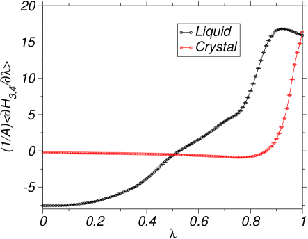
Figure 3: Thermodynamic integrand corresponding to steps 3 and 4, for the liquid and (100) orientation of the crystal, respectively, at the temperature $T=1.0$.

In Fig. 3, thermodynamic integrands corresponding to steps 3 and 4 are shown. We obtained excellent overlap between the forward and reverse thermodynamic integrand curves and therefore only data corresponding to the forward transformation is reported. For step 3, hysteresis between the forward and reverse TI calculations was less than $0.005k_{\rm B}T$, while for step 4 the same was less than $0.001k_{\rm B}T$ for all the three orientations.

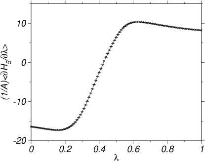
Figure 4: Thermodynamic integrand for step 5 at $T=1.0$, bringing the (100) orientation of the crystal in contact with the liquid.

At the end of step 3, the liquid is ordered into crystalline layers near the interface. Therefore, the structured wall induces precrystallization of the liquid even at the bulk liquid coexistence density heniloewenjpcm . Since the liquid is already ordered into a structure compatible with the crystal, the next transformation, step 5, corresponding to joining the liquid and crystal phases, occurs smoothly as shown in Fig. 4. The hysteresis between the forward and reverse TI paths was less than $0.007{k_{\rm B}}T$ for the various orientations and system-sizes specified in Table I.

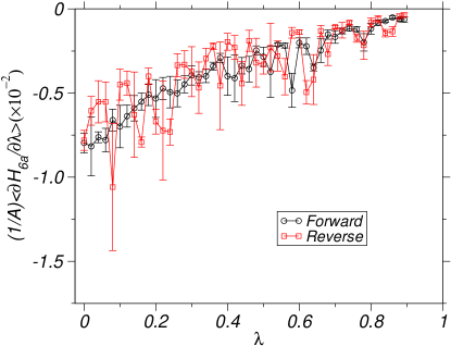
Figure 5: Thermodynamic integrands for the forward and reverse processes corresponding to step 6a, towards reducing the range of the flat wall.

The final step consists of two sub-steps. In step 6a, we reduce the range of the Gaussian flat wall to an extremely small value. As specified in Section III, the parameter $b$ was changed from $0.027\sigma$ [corresponding to a range of $0.1\sigma$ with the range considered to be the distance at which $u_{fw}(z_{\rm iw})$ decays to about $0.0001k_{\rm B}T$] to $0.0003\sigma$ (corresponding to a range of about $0.001\sigma$). For this range of the potential, the free-energy difference per unit area of a liquid in contact with this flat wall was $0.0005k_{\rm B}T$ and for the various orientations of the crystal is less than $0.00002k_{\rm B}T$. Clearly, reducing the range of the flat wall by about $100$ times also reduces the free-energy difference by about the same factor.

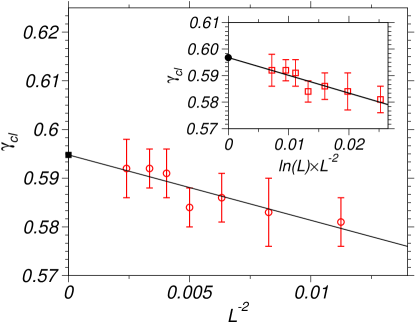
Figure 6: $\gamma_{\rm cl}$ as a function $1/L^{2}$, where $L=L_{\rm x}=L_{\rm y}$, for (100) orientation of the crystal-liquid interface with the longitudinal dimension $2L_{\rm z}=78.58\,\sigma$. Inset shows $\gamma_{\rm cl}$ as a function of  $\ln(L)/L^{2}$. Solid symbols correspond to the $\gamma_{\rm cl}$ values in the thermodynamic limit.

Orientation	N	System Size	$\gamma_{\rm cl}^{\rm inv}$	$\gamma_{\rm cl}^{\rm HS}$	Cleaving (HS)	Cleaving (IP)
$100$	$6860$	$9.43\times 9.43\times 78.58$	$0.581\pm 0.005$	$0.585\pm 0.005$	—	—
$100$	$9338$	$11.0\times 11.0\times 78.58$	$0.584\pm 0.007$	$0.588\pm 0.007$	—	—
$100$	$12196$	$12.57\times 12.57\times 78.58$	$0.586\pm 0.005$	$0.590\pm 0.005$	—	—
$100$	$15436$	$14.15\times 14.15\times 78.58$	$0.584\pm 0.004$	$0.588\pm 0.004$	—	—
$100$	$19056$	$15.72\times 15.72\times 78.58$	$0.591\pm 0.005$	$0.595\pm 0.005$	—	—
$100$	$23058$	$17.29\times 17.29\times 78.58$	$0.592\pm 0.004$	$0.596\pm 0.004$	—	—
$100$	$32205$	$20.43\times 20.43\times 78.58$	$0.592\pm 0.006$	$0.596\pm 0.006$	$0.5820\pm 0.0019$	$0.592\pm 0.007$
$100$	$\infty$	$\infty$	$0.595^{\rm a},0.597^{\rm b}$	$0.599^{\rm a},0.601^{\rm b}$	—	—
$110$	$32106$	$20.43\times 20.0\times 80.02$	$0.573\pm 0.004$	$0.577\pm 0.004$	$0.5590\pm 0.0020$	$0.571\pm 0.006$
$111$	$33959$	$21.17\times 20.0\times 81.66$	$0.552\pm 0.003$	$0.556\pm 0.003$	$0.5416\pm 0.0031$	$0.557\pm 0.007$

Table 1: Interfacial free energy $\gamma_{\rm cl}^{\rm inv}$ for different system sizes corresponding to various orientations of the crystal-liquid interface. The interfacial free-energies for the pure hard-sphere system obtained by using a scaling parameter are also shown (see text). For comparison, data from the cleaving wall methods for the pure hard-sphere (HS) system davidchack2010 and for the inverse power-law (IP) potential in the hard-sphere limit laird-davidchack2005prl are also reported. Dimensions ($L_{\rm x}\times L_{\rm y}\times L_{\rm z}$) are in units of $\sigma^{3}$. For the (100) orientation of the crystal-liquid interface, the interfacial free energy in the thermodynamic limit is extrapolated from the values of $\gamma_{\rm cl}$ at the various system sizes using the (a) $L^{-2}$ and (b) $\ln(L)L^{-2}$ scalings (see text).

In step 6a, the range of the potential was modified by varying $\lambda$ from $0$ to $0.894$. At $\lambda=1.0$, the range of the flat wall would be zero. Clearly, to chose an appropriate final value of $\lambda$ in step 6a, the strategy would be to first compute the accumulated free energy difference up to step 5. Depending upon the desired accuracy, a value is chosen which is much less than the statistical and numerical errors in the combined steps 1-5. From the ratio of this value and $\Delta F_{\rm 1}/A$, a factor is obtained and multiplying it with the range of the flat-wall potential in step 1, a new range can be calculated, from which the appropriate final value of $\lambda$ in step 6a can be deduced from Eq. 3. By this strategy, step 6b would become redundant as argued in Section III.

In Fig. 5, we plot the thermodynamic integrands corresponding to the forward and reverse paths of step 6a. Though the curves are a bit noisy compared to the previous steps, the magnitude of the integrands are also very small and hysteresis between the forward and reverse calculations is $0.0005k_{\rm B}T$, while ${\Delta F_{\rm 6a}}/A=-0.003k_{\rm B}T$. For the (110) and (111) orientations, the contribution from step 6a is, $-0.020\pm 0.001$ and $-0.002\pm 0.001$, in units of $k_{\rm B}T/\sigma^{2}$.

We have carried out several independent runs corresponding to step 6b and from the runs with the least hysteresis, we extracted the free-energy difference. However, for all the three orientations the magnitude of the contribution was less than $0.0005k_{\rm B}T/\sigma^{2}$ and hence the thermodynamic integrands are not shown and neither were they added to the final value of $\gamma_{\rm cl}$.

The final value of $\gamma_{\rm cl}$ after adding the contributions from each step is reported in Table I for the three orientations and for various system sizes corresponding to the (100) orientation. Using the scaling parameter $\sigma^{\rm eff}=1.0035\sigma$, the equivalent interfacial free-energy for the hard-sphere potential is also specified. Data from the cleaving-wall method corresponding to the pure hard-sphere potential davidchack2010 and that for the inverse-power potential extrapolated to the hard-sphere limit ($n\rightarrow\infty$) laird-davidchack2005prl is also reported. While our results are slightly higher than those obtained for the former case, they are in good agreement with the later, within the reported errors. Another TI approach reported recently yielded a similar value for the (100) orientation of the hard-sphere crystal-liquid interface espinosa2014 .

To study systematic errors arising from finite-size effects we have carried out simulations for the (100) orientation of the crystal-liquid interface at various lateral dimensions ($L_{\rm x}\times L_{\rm y}$) keeping the longitudinal dimension fixed at $78.58\,\sigma$. Recently, Schmitz et al. schmitz2014 identified the finite-size corrections and proposed a scaling relation to obtain reliable estimates for the interfacial free energies in the thermodynamic limit. According to them, the leading finite size corrections to the interfacial free energy in the thermodynamic limit is described by the following relation schmitz2014 ; binder82 :

$$\gamma_{\rm L,L_{\rm z}}=\gamma_{\rm\infty}-A\frac{\ln L_{\rm z}}{L^{2}}+B\frac{\ln L}{L^{2}}+\frac{C}{L^{2}}\,$$ (14)

where $A$, $B$ and $B$ are constants and $L=L{\rm x}=L_{\rm y}$ corresponds to the lateral dimension of our system.

The second term in Eq. (14) is identified with the translational entropy of the system arising from the movement of the crystal-liquid interface. Since, the flat walls restrict the movement of the crystal-liquid interface, this term can be neglected in our TI scheme. In Fig. 6, we plot $\gamma_{\rm cl}$ as a function of $1/L^{\rm 2}$ and $\ln(L)/L^{\rm 2}$ separately. Extrapolating the data linearly yields $\gamma_{\rm cl}$, the equivalent hard-sphere crystal-liquid interfacial free energy in the thermodynamic limit and for the $1/L^{\rm 2}$ and $\ln(L)/L^{\rm 2}$ scalings we obtain the values $0.599k_{\rm B}T/{\sigma}^{2}$ and $0.601k_{\rm B}T/{\sigma}^{2}$, respectively.

In comparison to the values of $\gamma_{\rm cl}$ corresponding to the smallest system sizes considered, the thermodynamic limit value is around $3\%$ higher, indicating that finite-size corrections cannot be ignored in order to obtain a reliable estimate. The linear scaling observed in Fig. 6 also indicates that capillary fluctuations are not suppressed on account of the flat walls. It is also to be noted that values of $\gamma_{\rm cl}$ obtained in the thermodynamic limit for the (100) orientation of the crystal-liquid interface are about $6-7\%$ less than those corresponding to the capillary fluctuation hartel2012 and tethered Monte Carlo approach martin2012 . More research is needed to understand the origin of this discrepancy.

VI Conclusion

We have obtained the crystal-liquid interfacial free energy for the hard sphere system via a novel thermodynamic integration scheme. Good agreement of our results with other computational approaches indicates the success of our TI scheme even for short-ranged interaction potentials. The flat Gaussian walls introduced in this scheme circumvents the problem of achieving a reversible transformation due to the movement of the crystal-liquid interface. These flat walls suppress the movement of this interface and at the same time do not affect the capillary fluctuations. Use of frozen-in crystalline layers to act as structured walls induces ordering in the liquid compatible with the crystal structure and leads to a smooth thermodynamic transformation to the desired final state.

Our results also indicate that finite-size errors have to be accounted for in order to obtain accurate estimates for $\gamma_{\rm cl}$. The accurate values for the interfacial free energy obtained in this work can be used to validate future DFT approaches, which in the past have yielded higher values as compared to a TI calculation hartel2012 . Furthermore, a TI calculation of $\gamma_{\rm cl}$ using our scheme is necessary for the pure hard sphere system to be able to compare with existing values. Work along these lines is currently under way.

Acknowledgments:
The authors acknowledge financial support by the German DFG SPP 1296, Grant No. HO 2231/6-3.

References

- (1) B. J. Alder and T. E. Wainright, J. Chem. Phys. 27, 1208 (1957).
- (2) A. Mulero, Theory and Simulation of Hard-Sphere Fluids and Related Systems, Lecture Notes in Physics 753 (Springer, Berlin, 2008).
- (3) S. Auer and D. Frenkel, Nature 409, 1020 (2001).
- (4) M. Amini and B. B. Laird, Phys. Rev. Lett. 97, 216102 (2006).
- (5) T. Zykova-Timan, R. E. Rozas, J. Horbach, and K. Binder, J. Phys.: Condens. Matter 21, 464102 (2009).
- (6) T. Zykova-Timan, J. Horbach, and K. Binder, J. Chem. Phys. 133, 014705 (2010).
- (7) L. Filion, M. Hermes, R. Ni, and M. Dijkstra, J. Chem Phys. 133, 244115 (2010).
- (8) W. A. Curtin, Phys. Rev. B 39, 6775 (1989).
- (9) D. W. Marr and A. P. Gast, Langmuir 10, 1348 (1994).
- (10) D. W. Marr, J. Chem. Phys. 102, 8283 (1995).
- (11) T. Gruhn and P. Monson, Phys. Rev. E 64, 061703 (2001).
- (12) B. O’Malley and I. K. Snook, Phys. Rev. Lett. 90, 085702 (2003).
- (13) E. Zaccarelli, C. Valeriani, E. Sanz, W. C. K. Poon, M. E. Cates, and P. N. Pusey, Phys. Rev. Lett. 103, 135704 (2009).
- (14) T. Kawasaki and H. Tanaka, Proc. Nat. Acad. Sci. 107, 14036 (2010).
- (15) T. Schilling, H.-J. Schöpe, M. Oettel, G. Opletal, and I. K. Snook, Phys. Rev. Lett. 105, 025701 (2010).
- (16) A. W. Adamson and A. P. Gast, Physical chemistry of surfaces (Wiley-Interscience, New York, 1997).
- (17) D. Turnbull and R. E. Cech, J. Appl. Phys. 21, 804 (1950).
- (18) D. Turnbull, J. Appl. Phys. 21, 1022 (1950).
- (19) D. Turnbull, J. Chem. Phys. 20, 411 (1952).
- (20) D. Woodruff, The Solid-Liquid Interface, 1st ed. (Cambridge University Press, London, 1973).
- (21) W. A. Tiller, The Science of Crystallization: Microscopic Interfacial Phenomena (Cambridge University Press, New York, 1991).
- (22) R. L. Davidchack and B. B. Laird, Phys. Rev. Lett. 85, 4751 (2000).
- (23) A. Cacciuto, S. Auer, and D. Frenkel, J. Chem. Phys. 119, 7467 (2003).
- (24) R. L. Davidchack and B. B. Laird, Phys. Rev. Lett. 94, 086102 (2005).
- (25) B. B. Laird and R. L. Davidchack, J. Phys. Chem. B 109, 17802 (2005).
- (26) R. L. Davidchack, J. R. Morris, and B. B. Laird, J. Chem. Phys. 125, 094710 (2006).
- (27) R. L. Davidchack, J. Chem. Phys. 133, 234701 (2010).
- (28) A. Härtel, M. Oettel, R. E. Rozas, S. U. Egelhaaf, J. Horbach, and H. Löwen, Phys. Rev. Lett. 108, 226101 (2012).
- (29) L. A. Fernandez, V. Martin-Mayor, B. Seoane, and P. Verrocchio, Phys. Rev Lett. 108, 165701 (2012).
- (30) T. P. Straatsma, M. Zacharias, and J. A. MacCammon, Computer Simulations of Biomolecular Systems (Escom, Keiden, 1993).
- (31) D. Frenkel and B. Smit, Understanding Molecular Simulation (Academic, San Diego, 2002).
- (32) R. L. Davidchack and B. B. Laird, Phys. Rev. E 54, R5905 (1996).
- (33) R. L. Davidchack and B. B. Laird, J. Chem. Phys. 118, 7651 (2003).
- (34) F. Schmitz, P. Virnau, and K. Binder, Phys. Rev. Lett. 112, 125701 (2014); ibid., Phys. Rev. E 90, 012128 (2014).
- (35) R. Benjamin and J. Horbach, J. Chem. Phys. 141, 044715 (2014).
- (36) D. C. Rapaport, The Art of Molecular Dynamics Simulation (Cambridge University Press, Cambridge, 2004).
- (37) K. Binder, Phys. Rev. A 25, 1699 (1982).
- (38) E. Lange, J. B. Caballero, A. M. Puertas, and M. Fuchs, J. Chem. Phys. 130, 174903 (2009).
- (39) J. Q. Broughton and G. H. Gilmer, J. Chem. Phys. 84, 5759 (1986).
- (40) R. Benjamin and J. Horbach, J. Chem. Phys. 137, 044707 (2012); J. Chem. Phys. 139, 039901 (2013).
- (41) R. Benjamin and J. Horbach, J. Chem. Phys. 139, 084705 (2013).
- (42) M. P. Allen and D. J. Tildesley, Computer Simulations of Liquids (Clarendon, Oxford, 1987).
- (43) P. Kuhn and J. Horbach, Phys. Rev. B 87, 014105 (2013).
- (44) R. Rozas, R. Benjamin, and J. Horbach, (manuscript in preparation).
- (45) M. Heni and H. Löwen, J. Phys.: Condens. Matter, 13, 4675 (2001).
- (46) J. R. Espinosa, C. Vega, and E. Sanz, J. Chem. Phys. 141, 134709 (2014).