String tension from smearing and Wilson flow methods

Abstract:

Recently, we proposed a new method to extract the string tension from 4-dimensionally smeared Wilson loops. In this talk, we first show that the results obtained using this smearing method are identical to those obtained by Wilson flow, once the time step is sufficiently small. We then demonstrate the practical advantage of our method by applying it to the calculation of string tension in SU(3) Yang-Mills theory.

1 Introduction

It is well known that Wilson loops of large size are quite noisy. The usual way to circumvent this difficulty is to apply 3-dimensional smearing to spatial link variables, and string tensions are then extracted from the smeared $q{\bar{q}}$ potential [1]. Recently, we proposed a new method to calculate string tension from 4-dimensionally smeared Wilson loops [2, 3]. The string tension is extracted directly from the continuum limit of Creutz ratios.

Recently, Wilson flow became a standard technique to regularize local operators in which local link variables are evolved along fictitious time $t$ [4]. Link variables at $t$ are essentially the average of the original link variables in a spherical region of size $\sqrt{8t}$ in 4-dimensional space-time. Thus, by definition, Wilson flow is closely related to the 4-dimensional smearing method [5].

In this talk we first explain our 4-d smearing method, and then demonstrate that the same results are obtained when using Wilson flow instead, provided that the time step $\Delta t$ of the numerical time evolution is sufficiently small. Previously the method was used in the context of extracting the string tension for the large N limit of SU(N) gauge theory, and comparing it with the result of reduced models [6, 7]. Here we will apply it to SU(3) Yang-Mills theory. To test the scaling of the results we will study three different values of the coupling while keeping constant the physical size of the box. Apart from the string tension we will also obtain a continuum function built in terms of Wilson loops. We will then compare our results to those obtained from spatially smeared $q{\bar{q}}$ potential.

2 4-dimensional Ape smearing

We consider 4-dimensional Ape smearing defined by [8, 5]

$$U_{n,\mu}^{smeared}={\rm Proj}_{SU(3)}\left[(1-f)U_{n,\mu}+{f\over 6}\sum_{\nu\neq\mu=\pm 1}^{\pm 4}U_{n,\nu}U_{n+\nu,\mu}U_{n+\mu,\nu}^{\dagger}\right],$$ (1)

where ${\rm Proj}_{SU(3)}$ stands for the operator for projection onto the SU(3) matrices. As explained in Ref. [5], for sufficiently small steps $\Delta t=f/6$ the smearing procedure should scale with the variable $t=fn_{s}/6$, where $n_{s}$ denotes the number of smearing steps. In the next section, we will show that the same results are obtained from Wilson flow at the fictitious time equal to $t$.

In the literature, it is customary to apply 3-dimensional Ape smearing to spatial link variables to obtain smeared $q{\bar{q}}$ potential with small noises [1]. On the other hand, 4-dimensional Ape smearing is not extensively used so far [9], because smeared Wilson loops and smeared $q{\bar{q}}$ potentials have huge $t$ dependences. As an example, In Fig. 2, we show the $t$ dependence of a Wilson loop and in Fig. 2, that of the discretized $q{\bar{q}}$ potential $V(R,T)=-\log\left[W(R,T+1/2)/W(R,T-1/2)\right]$ with integer $R$ and half-integer $T$. The simulation has been made on a $32^{4}$ lattice at $\beta=6.17$ with $f$=0.1. The smeared Wilson loops can be considered regulated versions with $t$ playing the role of an ultraviolet cut-off. The divergences of these quantities imply then a strong $t$ dependence as we approach the continuum limit.

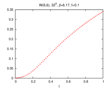
Figure 1: $t$ dependence of Wilson loop $W(6,6)$.

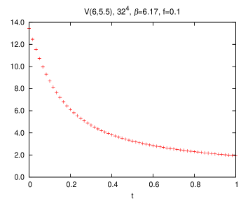
Figure 2: $t$ dependence of $q{\bar{q}}$ potential $V(6,5.5)$.

Our proposal is rather to consider Creutz ratios

$$\chi(R,T)=-\log{W(R+1/2,T+1/2)W(R-1/2,T-1/2)\over W(R+1/2,T-1/2)W(R-1/2,T+1/2)}$$ (2)

with half-integer $R$ and $T$. Since Creutz ratios $\chi(R,T)$ are free from ultraviolet divergences, we expect that the smeared quantities have a well defined $t\rightarrow 0$ limit. As an example, in fig. 4 we show $\chi(5.5,5.5)$ as a function of $t$ at $\beta=6.17$ with $f$=0.1. Notice however that, for small values of $t$, $\chi(R,T)$ has huge errors. This is understandable since the Creutz ratios are constructed in terms of the ultraviolet divergent quantities which are affected by large errors. On the other hand as we increase $t$, the error drops considerably. The $t$-dependence of Creutz ratios is understandable and computable in perturbation theory. Restricting ourselves to not too large values of $t$ this suggests a parameterization of the type

$$\chi(t)=a\left\{1-\exp\left({-b\over t+c}\right)\right\}.$$ (3)

which, as seen in fig. 4, perfectly fits the data. It is clear that around $t\sim 0.4$ the curve is essentially horizontal and its value gives a good estimate of the $t\rightarrow 0$ limit. However, to avoid fitting a constant within a subjective range, it is much better to use the previous functional form and fit also the values for $t>0.5$.

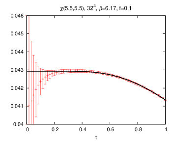
Figure 3: $t$ dependence of the 4-d smeared Creutz   
ratio $\chi(5.5,5.5)$. The solid line is the fit with (2.3).

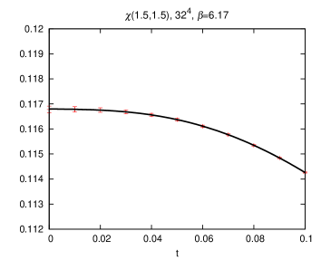
Figure 4: $t$ dependence of the 4-d smeared Creutz   
ratio $\chi(1.5,1.5)$. The solid line is the fit with (2.3).

For small loop sizes, Creutz ratios generally have small statistical errors. As an example, we show in fig. 4 the $t$ dependence of $\chi(1.5,1.5)$. The necessity of using smearing is then not clear. However, notice that the fit with (3) is indeed quite good. It should be noted that, for small loop sizes, the existence of the parameter $c$ is crucial to fit the data. The smeared Creutz ratio monotonically decreases as we increase $t$, implying that there is actually no plateau.

3 Relation with Wilson flow

As mentioned earlier the smearing dependence is actually better expressed in terms of $t$. This is clearly seen in Fig. 6 where results for three different values of $f$ are compared. We also analyzed the dependence of the result on the regulating method. For that purpose we applied Wilson flow with fictitious time $t$, defined by [4]

$$dV_{n,\mu}(t)/dt=-g_{0}^{2}\left\{\partial_{n,\mu}S_{W}\right\}V_{n,\mu}(t),\ \ \ V_{n,\mu}(t=0)=U_{n,\mu}.$$ (4)

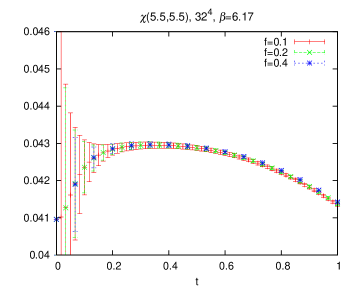
Figure 5: Smeared Creutz ratio with $f$=0.1, 0.2  
and 0.4.

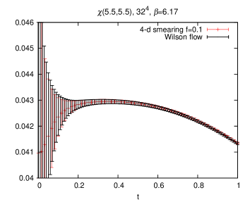
Figure 6: $\chi(5.5,5.5)$ from 4-d smearing (red symbol) and that from Wilson flow (black symbol).

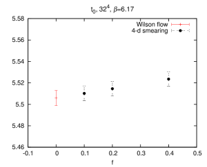
Figure 7: $f$ dependence of $t_{0}$.

We have used third-order Runge-Kutta scheme with $\Delta t=0.01$. In fig. 6, we compare the results obtained from 4-d smearing ($f$=0.1) with that from Wilson flow. It is obvious that both methods give identical values of the smeared Creutz ratios once the time step $f$ is sufficiently small. A slight $f$-dependence is observed when computing the scale $t_{0}$ defined by $\left\{t^{2}\left<E\right>\right\}_{t=t_{0}}$ = 0.3 [4], with $E$ evaluated from the lattice version of $F_{\mu\nu}$. The result is displayed in Fig. 7 and compared with the result obtained by Wilson flow. These slight discretization errors, however, do not affect the $t\rightarrow 0$ extrapolation of Creutz ratios.

Concerning the dependence of the parameters of the fit on the size of the loop, perturbation theory predicts that $b\sim 25/R^{2}$. Indeed, our data agrees with a dependence on $25/(R-0.5)^{2}$, which is consistent with this prediction up to discretization effects.

4 Application to SU(3) Yang-Mills theory

In order to demonstrate the practical usefulness of our method, we have applied it to the SU(3) Yang-Mills theory and calculated the string tension and the continuum version of the Creutz ratios for that case. To monitor scaling behaviour we have made simulations at three lattices having approximately equal physical size as shown in Table 1. The scale ${\bar{r}}$ was defined in Refs. [2, 3] and its definition will be given later. In this talk, we will concentrate on the diagonal Creutz ratios $\chi(R,T)$ with $R=T$, although there are a lot of interesting physics in off-diagonal $\chi(R,T)$ [2, 3].

Lattice	$\beta$	$N_{cnfg}$	$a/{\bar{r}}$	$t_{0}/a^{2}$	$\sqrt{8t_{0}}/{\bar{r}}$
$24^{4}$	5.96	1000	0.2117(5)	2.794(3)	1.001(2)
$32^{4}$	6.17	300	0.1499(2)	5.506(7)	0.995(2)
$48^{4}$	6.42	100	0.1052(3)	11.17(3)	0.994(3)

Table 1: Properties and statistics of three lattice runs.

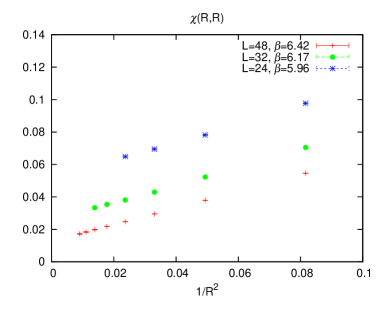
Figure 8: Creutz ratio $\chi(R,R)$ as functions of $1/R^{2}$.

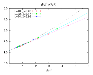
Figure 9: $({\bar{r}}/a)^{2}\chi(R,R)$ as functions of $({\bar{r}}/r)^{2}$.

In Fig. 9 we display the results obtained for the diagonal Creutz ratios $\chi(R,R)$ using the 4d smearing method described earlier. The statistical error are too small to be seen at the scale of the plot. To analyze scaling it is better to consider the quantity $R^{2}\chi(R,R)$ which in the continuum limit tends to a dimensionless function as follows:

$$R^{2}\chi(R,R)\stackrel{{\scriptstyle a\rightarrow 0}}{{\longrightarrow}}r^{2}{\tilde{F}}(r)+\mathcal{O}(\frac{a^{2}}{r^{2}})$$ (5)

where $r=Ra$. The function ${\tilde{F}}(r)$ can be written in terms of Wilson loops as follows:

$${\tilde{F}}(r)=-\lim_{t\rightarrow 0}\left.\frac{\partial^{2}\log W_{t}(r,r^{\prime})}{\partial r\partial r^{\prime}}\right|_{r=r^{\prime}}.$$ (6)

where $W_{t}(r,r^{\prime})$ is the continuum Wilson loop regulated with smearing parameter $t$. Although $\lim_{t\rightarrow 0}W_{t}(r,r^{\prime})$ is not well-defined, it is in the expression of ${\tilde{F}}(r)$. The scale $a(\beta)$ can be fixed by any method. However, one can use the information of the Creutz ratios themselves to obtain them in units of a new scale ${\bar{r}}$ (á la Sommer), defined by the equation ${\bar{r}}^{\ 2}\tilde{F}(\bar{r})=1.65$ [2, 3].

In applying the previous ideas to our data, we first realize that, in the range of $R$ values explored, the Creutz ratios can be perfectly fitted by a second degree polynomial in $1/R^{2}$. Combining this with the previous information we might write

$$\left({{\bar{r}}\over a}\right)^{2}\chi(R,R)=\sigma{\bar{r}}^{\ 2}+2\gamma\left({{\bar{r}}\over r}\right)^{2}+4\left({{\bar{r}}\over r}\right)^{4}\left[c+d\left({a\over{\bar{r}}}\right)^{2}\right]$$ (7)

in which we have allowed for a term (associated to the $d$ parameter) to account for the leading correction to scaling effects. Thus the continuum function ${\tilde{F}}(r)$ is described by

$${\bar{r}}^{\ 2}{\tilde{F}}(r)=\sigma{\bar{r}}^{\ 2}+2\gamma\left({{\bar{r}}\over r}\right)^{2}+4c\left({{\bar{r}}\over r}\right)^{4}$$ (8)

The definition of the scale ${\bar{r}}$ implies a relation among the parameters as follows

$${\bar{r}}^{\ 2}{\tilde{F}}({\bar{r}})=\sigma{\bar{r}}^{\ 2}+2\gamma+4c=1.65$$ (9)

which allow us to determine $c$ in terms of the other parameters. Summarizing, we are led to a simultaneous parameterization of the Creutz ratios for the three values of $\beta$ as follows

$$\left({{\bar{r}}\over a}\right)^{2}\chi(R,R)=\sigma{\bar{r}}^{\ 2}+2\gamma\left({{\bar{r}}\over a}\right)^{2}{1\over R^{2}}+4\left({{\bar{r}}\over a}\right)^{4}{1\over R^{4}}\left[{1.65-\sigma{\bar{r}}^{\ 2}-2\gamma\over 4}+d\left({a\over{\bar{r}}}\right)^{2}\right]$$ (10)

given in terms of 6 fitting parameters $\sigma{\bar{r}}^{\ 2},\ \gamma,\ d,\ {a(\beta=5.96)\over{\bar{r}}},\ {a(\beta=6.17)\over{\bar{r}}},\ {a(\beta=6.42)\over{\bar{r}}}.$ The fit has a reduced chi square of $\chi^{2}$/ndf=1.05, and the fitted parameters are

$$\sigma{\bar{r}}^{\ 2}=1.159(6),\ \gamma=0.250(3),\ d=0.24(2)$$ (11)

plus the values of $a/{\bar{r}}$ given in Table 1. In Fig. 9 we display the data together with the fitting function for the three values of $\beta$. Although the three curves and the data coalesce for large values of $r$, they are clearly different at smaller $r$. The difference is perfectly accounted for by the expected correction to scaling given in terms of the single parameter $d$. Using the measured value of this parameter we display in Fig. 10 the result for the continuum function $\bar{r}^{\ 2}\tilde{F}(r)$ obtained from our three values of beta. Scaling is almost perfect. Notice that the resulting function provides a continuum observable of pure gauge theory which had not been measured before.

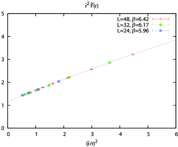
Figure 10: The continuum form of Creutz ratios ${\bar{r}}^{\ 2}{\tilde{F}}(r)$ plotted as a function of $({\bar{r}}/r)^{2}$.

The use of the new unit ${\bar{r}}$ has allowed us to give a self-contained determination of the continuum function. However, the ratio of scales $a(\beta=6.17)/a(6.42)=1.4249(45)$ is independent of the choice of units. This ratio matches perfectly with the result following from the formula of Ref. [10], which is $1.4252$. It also agrees within errors with the value given in Ref. [4]: $1.4310(24)$. The latter uses the unit $t_{0}$ mentioned earlier. We have also determined this quantity from our data. The results are given in Table 1. From it we deduce $a(6.17)/a(6.42)=1.4243(21)$. The agreement between our two determinations and those of other authors is remarkable. From it we can determine the ratio of length units $\sqrt{8t_{0}}/{\bar{r}}$ which averages to $0.995(5)$, and using $\sqrt{8t_{0}}/{r_{0}}=0.948(6)$ [4], obtain $\bar{r}/r_{0}$.

A similar test of scaling can be done by looking at the ratio $a(5.96)/a(6.17)$. One expects higher violations of scaling at this lower $\beta$ and indeed the results are not so spectacular, but well under the percent level. One gets $1.4123(21)$ from our fit, $1.4063$ from Ref. [10], $1.4038(24)$ from Ref. [4] and $1.4038(12)$ from our $t_{0}$ determination.

Using the length scale relations of the previous paragraphs we can transform our string tension measurement in Eq. 11 into other units. We get $\sqrt{8t_{0}\sigma}=1.071(6)$ and $r_{0}\sqrt{\sigma}=1.13(1)$. Previous measurements of this quantity derived from 3-d smeared potential are almost consistent with the value $r_{0}\sqrt{\sigma}=\sqrt{1.65-\pi/12}=1.178$ [1]. It is not clear how to interpret the 5% difference between the two values of $r_{0}\sqrt{\sigma}$, but in view of the previous results, it can hardly be due to errors in the scale determination. It should be noted, however, that the two numbers are obtained from quite different geometries of Wilson loops. In fact, for 3-d smearing, we use Wilson loop $W(R,T)$ with finite $R$ and infinite $T$, and the resultant expression of the force is $r_{0}^{2}F(r)=r_{0}^{2}\sigma+{\pi\over 12}\left({r_{0}\over r}\right)^{2}\simeq r_{0}^{2}\sigma+0.2612\left({r_{0}\over r}\right)^{2}$. On the other hand, for 4-d smearing, we use Wilson loop $W(R,T)$ with finite $R\approx T$, and the resultant expression of the Creutz Ratio is given in eq. (8).

In conclusion, we have presented a method based on 4-dimensional Ape smearing that allows a precise determination of Creutz ratios. We showed that the results are insensitive to using Wilson flow instead. The method is applied to SU(3) pure gauge theory allowing to compute a physical function of length which is the continuum equivalent of Creutz ratios, and whose large size limit is the string tension.

A.G-A acknowledges financial support from the grants FPA2012-31686 and FPA2012-31880, the MINECO Centro de Excelencia Severo Ochoa Program SEV- 2012-0249, the Comunidad Autónoma de Madrid HEPHACOS S2009/ESP-1473, and the EU PITN-GA-2009-238353 (STRONG net). He participates in the Consolider- Ingenio 2010 CPAN (CSD2007-00042). M. O. is supported by the Japanese MEXT grant No 26400249. Calculations have been done on the INSAM clusters at Hiroshima University and also on Hitachi SR16000 supercomputer both at High Energy Accelerator Research Organization(KEK) and YITP in Kyoto University. Work at KEK is supported by the Large Scale Simulation Program No.13/14-02.

References

- [1] For the compilation of 3-d smearing results, see for example, R. G. Edwards, U. M. Heller and T. R. Klassen, Accurate scale determinations for the Wilson gauge action, Nucl. Phys. B 517 (1998) 377 [arXiv:hep-lat/9711052].
- [2] A. Gonzalez-Arroyo and M. Okawa, The string tension for large N gauge theory from smeared Wilson loops, PoS LAT2012 (2012) 221 [arXiv:1212.3835 [hep-lat]].
- [3] A. Gonzalez-Arroyo and M. Okawa, The string tension from smeared Wilson loops at large N, Phys. Lett. B 718 (2013) 1524 [arXiv:1206.0049 [hep-th]].
- [4] M. Lüscher, Properties and uses of the Wilson flow in lattice QCD, JHEP 1008 (2010) 071 [arXiv:1006.4518 [hep-lat]].
- [5] R. Narayanan and H. Neuberger, Infinite N phase transitions in continuum Wilson loop operators, JHEP 0603 (2006) 064 [arXiv:hep-th/0601210].
- [6] A. Gonzalez-Arroyo and M. Okawa, Twisted Eguchi-Kawai model: A reduced model for large N lattice gauge theory, Phys. Rev. D 27 (1983) 2397.
- [7] A. Gonzalez-Arroyo and M. Okawa, Large N reduction with the Twisted Eguchi-Kawai model, JHEP 1007 (2010) 043 [arXiv:1005.1981 [hep-th]].
- [8] M. Albanese et al. (APE Collaboration), Glueball masses and string tension in lattice QCD, Phys. Lett. B192 (1987) 163.
- [9] See, however, R. Lohmayer and H. Neuberger, Rectangular Wilson loops at large N, JHEP 1208 (2012) 102 [arXiv:1206.4015 [hep-lat]].
- [10] M. Guagnelli, R. Sommer and H. Wittig, Precision computation of a low-energy reference scale in quenched lattice QCD, Nucl. Phys. B535 (1998) 389 [arXiv:hep-lat/9806005].