Transport in a harmonic trap: shortcuts to adiabaticity and robust protocols
Abstract
We study the fast transport of a particle or a Bose-Einstein condensate in a harmonic potential. An exact expression for the final excitation energy in terms of the Fourier transform of the trap acceleration is used to engineer optimal transport protocols (with no final excitation) that are robust with respect to spring-constant errors. The same technique provides a way to design the simultaneous and robust transport of a few non-interacting species that experience different harmonic trap frequencies in the same trap.
I Introduction
The accurate control of atomic motion is one of the goals of modern atomic, molecular, and optical (AMO) Physics. Neutral atoms and ions, individually, in condensates or in thermal clouds, are moved in many experimental settings from preparation to science chambers, to implement interferometers and metrological devices, or for quantum information operations among processing and storing sites. Atoms may simply be launched into free-flight or free-fall orbits, or be driven along moving traps. Moving traps offer the advantage of a more precise control that would let the atom, for example, start at rest and finish translationally unexcited, be stopped or accelerated, and perform curved trajectories in complex circuit geometries. Controlled atomic motion is a requisite for current and potential quantum technologies in which preserving quantum coherence and achieving high final fidelities with respect to target states is of paramount importance. Since the effects of noise and decoherence increase with process time, several groups have recently developed fast and robust transport protocols, shortcuts to adiabaticity (STA) reviewSTA13 , which are generically non-adiabatic but reproduce the final populations of an adiabatic transport process. They not only minimize the effects of noise but also allow for quick information processing or for more repetitions of the operation NIST06 ; David08 ; Calarco09 ; Masuda10 ; Erik11 ; transOCT12 ; Erikcond12 ; Masuda12 ; Mikel13 ; Adol14 ; Uli14 ; Lu14 . Several experiments have also demonstrated STA transport for different systems and conditions David08 ; Nice ; Bowler ; Walther .
The “robustness” mentioned before is a relative concept that depends on the type of perturbation that affects the ideal external driving Andreas ; AndreasPRL ; Lu14 . One of the basic problems that protocol design must face is the instability of the spring constant from run to run of the experiment, while keeping a constant value during each run. This may in fact be the dominant problem in some settings Lu14 . In this paper we address this difficulty by providing a protocol design strategy that imposes zeros of final excitation in a discrete set of spring constants. With an appropriate arrangement of points, broad trap-frequency windows for excitation-free fast transport may be achieved.
II Transport of a one-body wave function
The transport of a wave function of a particle of mass in a moving harmonic trap of angular frequency (spring constant ) is described, in an effectively one dimensional scenario, by the time-dependent Schrödinger equation
| (1) |
where and The scalar “transport function” denotes the position of the minimum of the harmonic potential and obeys the boundary conditions , , , and for a transport over a distance in a time interval , assuming that the trap starts and ends up at rest. In Appendix A we give the expression for the exact solution of Eq. (1) whatever is . This solution is related to the evolution of a fictitious classical particle of coordinate that obeys the equation of motion of the classical counterpart of the transport problem,
| (2) |
When the initial wave function is in the ground state, the energy at a time can be readily calculated from the solution (see Appendix B):
| (3) | |||||
If the goal is to avoid any excess energy, , the fictitious particle trajectory must obey the boundary conditions , , . By virtue of the equation fulfilled by , we have also , as is assumed to be continuous. This set of boundary conditions coincides with that obtained with the shortcut-to-adiabaticity method based on Lewis-Riesenfeld invariants Erik11 ; reviewSTA13 . The solution for the transport function is then constructed by an inverse-engineering method which consists in (i) choosing a function that obeys the appropriate set of boundary conditions, and (ii) then inferring from Eq. (2) the corresponding trajectory of the potential, .
As shown in Erikcond12 the wave function of a Bose-Einstein condensate satisfying a Gross-Pitaevskii equation in a moving external harmonic potential is shape invariant and the only possible excitations associated with such a mode are center of mass oscillations, along the classical trajectory in Eq. (2), with constant mean field energy. The same STA strategy as for the one-body wave function can therefore be used for the transport of a condensate.
III Transport without final excess energy at two trap frequencies
The optimal transport of a particle corresponds to the cancellation of the Fourier transform of the acceleration of the displacement of the trap, , at the trap angular frequency (see Appendix B):
| (4) |
Consider two angular frequencies and for which we would like the final state to have no excitation: . To design the appropriate acceleration function, , we introduce an auxiliary function such that
| (5) |
and which obeys the boundary conditions . The auxiliary function is defined through the differential equation (5) so that, after integrating by parts and taking into account these boundary conditions, the Fourier transform of the acceleration becomes the product of a polynomial in with the desired zeros by the Fourier transform of the auxiliary function:
| (6) |
The squared frequencies in imply zeros at positive and negative frequencies. The latter might seem to be superfluous, but they avoid imaginary factors in Eq. (5) and guarantee the reality of for real .
After designing and deducing via Eq. (5), we integrate this equation twice with the boundary conditions , , and to specify the transport function,
| (7) |
Those latter boundary conditions imply that
| (8) |
Consider for instance the following polynomial interpolation:
| (9) |
The normalization factor is deduced from the second condition in Eq. (8),
| (10) |
with
| (11) | |||||
where is the incomplete beta Euler function. The second and third factors in Eq. (9) guarantee the boundary conditions at the time edges and the fourth one provides the odd symmetry to satisfy the first integral condition in Eq. (8). We therefore obtain an exact analytical solution for the transport problem which fulfills exactly the desired boundary conditions.
Finally, note that it is possible to set . The effect is to increase (double) the multiplicity of the zero at which flattens the excitation energy at that point. Examples to illustrate this effect and its applications are worked out in the following section.
IV Robust protocols
Robust protocols can be designed by generalizing the previous idea. Suppose that we identify an angular frequency region in which the values of the trap frequencies corresponding to different runs of the experiment are distributed. We would like our transport protocol to provide excitation-free final states in this region. For this purpose, we choose angular frequencies , with , and . The function should have now vanishing boundary conditions:
| (12) |
where . For instance, we can use the following simple polynomial interpolation, . The normalization factor is determined in the same manner as previously, see Eq. (10), with
| (13) | |||||
The desired form of the Fourier transform is
| (14) |
As
| (15) |
where
| (16) |
we can infer the link between the acceleration and the auxiliary function :
| (17) |
where we have used that
| (18) |
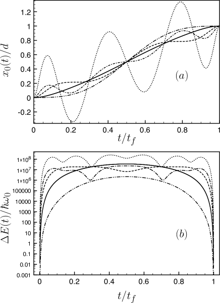
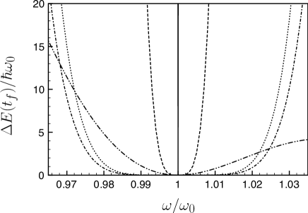
due to the boundary conditions (12). As in Sec. III, it is also possible to flatten the excitation energy curve versus around by increasing the multiplicity of the zero, i.e., simply choosing . In Fig. 1, we compare the one, two, and three frequency protocols with the choice . We have plotted both the trajectory and the transient excess of total energy during the transport. The parameters chosen for Fig. 1 are inspired by Ref. Walther in which a transport of single 40Ca+ ions is performed over a distance 20000 where is the harmonic length associated with the angular frequency MHz, in a time . We have chosen for Fig. 1 the same atom and angular frequency but have considered a transport over a larger distance, , realized over a much shorter time duration such that .
We clearly observe in Fig. 2 an impressive increase of the robustness against the variations of about through the increasing local flatness about when increases. A price to pay to benefit from this robustness is a more involved trap trajectory with a clear non monotonous character (Fig. 1a) and with an increasingly large transient energy (Fig. 1b) footnote . The oscillatory character of the trajectory can be intuitively understood. Indeed to ensure an optimal transport even for a trap frequency slightly smaller or larger than , one has to design a trajectory that compensates for the delay or advance that the two types of trapping about will imply. Such strategies are reminiscent of the spin echo technique in which a succession of pulses is used to focus the spins towards the desired state even though they experience different Rabi frequencies Molmer .
The performance of the protocols can be evaluated by means of the function
| (19) |
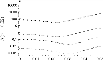
which gives the average excitation number over a finite range of frequencies about the central angular frequency . It therefore measures the robustness of the transport against the frequency of the trap. Figure 3 compares the performance of the 1,2 and 3-point protocols for and for two different final times. The abscissa measures the interval between chosen frequencies for 2 and 3 points, see the Figure caption. If not stated otherwise, the parameters for Fig. 3 are the same as for Fig. 1.
The observed general trends are intuitive: for a given protocol increasing the final time improves the robustness, the -point protocol yields an improvement by more than two orders of magnitude compared to the -point protocol. For the shortest transport time, the optimal choice for the 3-point protocol improves the robustness of the transport by more than five orders of magnitude compared to the 1-point protocol. Figure 3 also demonstrates the importance of the choice of the trap frequencies and the optimal intervals. This optimization shows that the protocol that relies on the same frequencies is never the best strategy. For instance, the three-point protocol with , and reduces the average excitation energy by a factor of more than 5 compared to the 3-point protocol with .
V Discussion
We have designed systematic fast transport protocols to leave the atoms (isolated, or in condensates) translationally unexcited at final time for a range of trap frequencies. This is instrumental in avoiding the effect of instability of trap frequencies among different runs of the experiment. Compared to a previous method (perturbative with respect to the spring constant deviations) to robustify the transport function Lu14 , the current approach is simpler to implement, contains no approximations, and gives an explicit form for the transport function for a chosen trap-frequency domain of stability. The same methods put forward here may be applied to other systems as well. Consider in particular two particles 1 and 2 confined by two different harmonic potentials with angular frequency and respectively. For instance, two different atoms in the same dipole trap or two atoms of the same species but in different Zeeman state that are magnetically trapped. We assume that the two particles do not interact. To transport optimally such a dual species system, we need to guarantee a vanishing energy excess for both types of atoms. The results of the 2-point protocol developed in Sec. III can then be applied directly. Its robustness can also be improved using higher order protocols as explained in the previous section. The technique to design optimal and robust trap trajectories can be readily generalized to more than two species following directly Sec. IV. Finally, the method described may also be applied to a broader set of physical inverse problems, e.g. in optics, to nullify the Fourier transform of a controllable function in a given interval.
Acknowledgements.
It is a pleasure to thank An Shuoming of Tsinghua University, and Xi Chen and Qi Zhang of Shanghai University for useful comments. This study has been partially supported through the grant NEXT ANR-10-LABX-0037 in the framework of the Programme des Investissements d Avenir and the Institut Universitaire de France. We also acknowledge funding by Basque Country Government (Grant No. IT472-10), Ministerio de Economía y Competitividad (Grant No. FIS2012-36673-C03-01), and the program UFI 11/55.Appendix A Exact solution
To find the exact solution of Eq. (5) we search for a solution of the form Husimi ; NIST06
| (20) |
where is a time dependent variable, and is the position shifted by a scalar time dependent parameter to be determined. In the following we show how and are related self-consistently. For this purpose, we calculate separately the different terms of the time-dependent Schrödinger solution:
| (21) | |||||
| (23) | |||||
Combining Eqs. (21), (23) and (23), we obtain
| (24) | |||||
By setting to zero the factor of and also the factor of we get the relation between and , and the equation of motion of the variable : . The variable corresponds to the trajectory of the classical counterpart of the quantum transport problem. The last term of Eq. (24) is a scalar time dependent term which contributes as a time dependent phase. To remove it we introduce the wave function defined by
| (25) |
where is the classical-mechanical Lagrangian of the transport,
| (26) |
With this choice, the wave function obeys the time dependent Schrödinger equation for a static harmonic potential of angular frequency ,
| (27) |
Finally, the exact expression for the solution of Eq. (5) takes the form
| (28) |
Appendix B Energy
The instantaneous energy reads . To perform this calculation using the solution (28), it is convenient to write the potential in the form . As is quadratic there are three contributions to the energy:
| (29) | |||||
Assuming that the initial state corresponds to the n-th eigenstate of the harmonic potential, we have with and the last integral of Eq. (29) vanishes by parity. The first term can be readily calculated. We thus find
| (30) |
Let us introduce the position of the fictitious classical particle in the frame of the moving potential. This position obeys the equation
| (31) |
The solution of this equation provided that and reads
| (32) |
Interestingly, we can write this solution in the complex form
| (33) |
The instantaneous energy can be also reexpressed in terms of :
| (34) |
For the transport problem we are interested in NIST06
| (35) |
In terms of dimensionless variables for time and trap-position:
| (36) |
where is the characteristic length for the harmonic oscillator, the excitation energy in units of the vibrational quantum takes the simple form
| (37) |
where and the double prime represents the second derivative with respect to .
Equation (35) provides us with an analogy between transport and Fraunhofer diffraction in optics. Indeed, the excess of energy is proportional to the modulus of the Fourier transform of the acceleration profile at the angular frequency . The acceleration profile therefore plays the role of an optical transmittance. According to this analogy, an optimal transport corresponds to a dark fringe in wave optics (zero intensity) David08 .
References
- (1) E. Torrontegui, S. Ibáñez, S. Martínez-Garaot, M. Modugno, A. del Campo, D. Guéry-Odelin, A. Ruschhaupt, Xi Chen, and J. G. Muga, Adv. Atom. Mol. Opt. Phys. 62, 117 (2013).
- (2) A. Couvert, T. Kawalec, G. Reinaudi, and D. Guéry-Odelin, Eur. Phys. Lett. 83, 13001 (2008).
- (3) M. Murphy, L. Jiang, N. Khaneja, and T. Calarco, Phys. Rev. A 79, 020301(R) (2009).
- (4) S. Masuda and K. Nakamura, Proc. R. Soc. A 466, 1135 (2010).
- (5) E. Torrontegui, S. Ibáñez, Xi Chen, A. Ruschhaupt, D. Guéry-Odelin, and J. G. Muga, Phys. Rev. A 83, 013415 (2011).
- (6) X. Chen, E. Torrontegui, D. Stefanatos, J.-S. Li, and J. G. Muga, Phys. Rev. A, 84, 043415 (2011).
- (7) E. Torrontegui, X. Chen, M. Modugno, S. Schmidt, A. Ruschhaupt, and J. G. Muga, New J. Phys. 14, 013031 (2012).
- (8) S. Masuda, Phys. Rev. A 86, 063624 (2012).
- (9) M. Palmero, E. Torrontegui, D. Guéry-Odelin, and J. G. Muga, Phys. Rev. A 88, 053423 (2013).
- (10) S. Deffner, C. Jarzynski, and A. del Campo, Phys. Rev. X 4, 021013 (2014).
- (11) H. A. Fürst, M. H. Goerz, U. G. Poschinger, M. Murphy, S. Montangero, T. Calarco, F. Schmidt-Kaler, K. Singer, C. P. Koch, New J. Phys. 16, 075007 (2014).
- (12) X.-J. Lu, J. G. Muga, X. Chen, U. G. Poschinger, F. Schmidt-Kaler, and A. Ruschhaupt, Phys. Rev. A 89, 063414 (2014).
- (13) R. Reichle, D. Leibfried, R. B. Blakestad, J. Britton, J. D. Jost, E. Knill, C. Langer, R. Ozeri, S. Seidelin, and D. J. Wineland, Fortschr. Phys. 54, 666 (2006).
- (14) J. F. Schaff, X. L. Song, P. Capuzzi, P. Vignolo, and G. Labeyrie, EPL 93, 23001 (2011).
- (15) R. Bowler, J. Gaebler, Y. Lin, T. R. Tan, D. Hanneke, J. D. Jost, J. P. Home, D. Leibfried, and D. J. Wineland, Phys. Rev. Lett. 109, 080502 (2012).
- (16) A. Walther, F. Ziesel, T. Ruster, S. T. Dawkins, K. Ott, M. Hettrich, K. Singer, F. Schmidt-Kaler, and U. Poschinger, Phys. Rev. Lett. 109, 080501 (2012).
- (17) A. Ruschhaupt, X. Chen, D. Alonso, and J. G. Muga, New J. Phys. 14, 093040 (2012).
- (18) D. Daems, A. Ruschhaupt, D. Sugny, and S. Guérin, Phys. Rev. Lett. 111, 050404 (2013).
- (19) I. Roos and K. Molmer, Phys. Rev. A 69, 022321 (2004).
- (20) K. Husimi, Prog. Theor. Phys. 9, 381 (1953).
- (21) For a transport over a distance in an amount of time , the maximum of the transient energy normalized to scales as Erik11 .