Abstract

In software engineering, taking a good election between recursion and iteration is essential because their efficiency and maintenance are different. In fact, developers often need to transform iteration into recursion (e.g., in debugging, to decompose the call graph into iterations); thus, it is quite surprising that there does not exist a public transformation from loops to recursion that handles all kinds of loops. This article describes a transformation able to transform iterative loops into equivalent recursive methods. The transformation is described for the programming language Java, but it is general enough as to be adapted to many other languages that allow iteration and recursion. We describe the changes needed to transform loops of types while/do/for/foreach into recursion. Each kind of loop requires a particular treatment that is described and exemplified.

1 Introduction

Iteration and recursion are two different ways to reach the same objective. In some paradigms, such as the functional or logic, iteration does not even exist. In other paradigms, e.g., the imperative or the object-oriented paradigm, the programmer can decide which of them to use. However, they are not totally equivalent, and sometimes it is desirable to use recursion, while other times iteration is preferable. In particular, one of the most important differences is the performance achieved by both of them. In general, compilers have produced more efficient code for iteration, and this is the reason why several transformations from recursion to iteration exist (see, e.g., [6, 9, 10]). Recursion in contrast is known to be more intuitive, reusable and debuggable. In fact, other researchers have obtained both theoretical and experimental results showing significant performance benefits of recursive algorithms on both uniprocessor hierarchies and on shared-memory systems [12]. In particular, Gustavson and Elmroth [4, 3] have demonstrated significant performance benefits from recursive versions of Cholesky and QR factorization, and Gaussian elimination with pivoting.

Transforming loops to recursion is also useful in debugging, as demonstrated by the technique presented in [8]. In this paper, transforming all iterative loops into recursive methods before starting an algorithmic debugging session can improve the interaction between the debugger and the programmer, and it can also reduce the granularity of the errors found. In particular, algorithmic debuggers only report buggy methods. Thus, a bug inside a loop is reported as a bug in the whole method that contains the loop, which is sometimes too imprecise. Transforming a loop into a recursive method allows the debugger to identify the recursive method (and thus the loop) as buggy. Hence, we wanted to implement this transformation and integrate it in the Declarative Debugger for Java (DDJ) [7], but, surprisingly, we did not find any available transformation from iterative loops into recursive methods for Java (neither for any other object-oriented language). Therefore, we had to implement it by ourselves and decided to automatize and generalize the transformation to make it publicly available. From the best of our knowledge this is the first transformation for all kinds of iterative loops.

One important property of our transformation is that it always produces tail recursive methods [2]. This means that they can be compiled to efficient code because the compiler only needs to keep two activation records in the stack to execute the whole loop [5, 1]. Another important property is that each iteration is always represented with one recursive call. This means that a loop that performs 100 iterations is transformed into a recursive method that performs 100 recursive calls. This equivalence between iterations and recursive calls is very important for some applications such as debugging, and it produces code that is more maintainable.

In the rest of the paper we describe our transformation for all kinds of loops in Java (i.e., while/do/for/foreach). The transformation of each particular kind of loop is explained with an example. We start with an illustrative example that provides the reader with a general view of how the transformation works.

Example 1

Consider the Java code in Algorithm 1 that computes the square root of the input argument.

Algorithm 1 Sqrt (iterative version)

1:  public double sqrt(double x) {

2:      if (x $<$ 0)

3:          return Double.NaN;

4:      double b = x;

5:      while (Math.abs(b * b - x) $>$ 1e-12)

6:          b = ((x / b) + b) / 2;

7:      return b;

8:  }

This algorithm implements a while-loop where each iteration obtains a more accurate approximation of the square root of variable x. The transformed code is depicted in Algorithm 2 that implements the same functionality but replacing the while-loop with a new recursive method $sqrt\_loop$.

Algorithm 2 Sqrt (recursive version)

1:  public double sqrt(double x) {

2:      if (x $<$ 0)

3:          return Double.NaN;

4:      double b = x;

5:      if (Math.abs(b * b - x) $>$ 1e-12)

6:          b = this.sqrt_loop(x, b);

7:      return b;

8:  }

9:  private double sqrt_loop(double x, double b) {

10:      b = ((x / b) + b) / 2;

11:      if (Math.abs(b * b - x) $>$ 1e-12)

12:          return this.sqrt_loop(x, b);

13:      return b;

14:  }

Essentially, the transformation performs two steps:

1. Substitute the original loop by new code (lines 5-6 in Algorithm 2).

2. Create a new recursive method (lines 9-14 in Algorithm 2).

In Algorithm 2, the new code in method $sqrt$ includes a call (line 6) to the recursive method $sqrt\_loop$ that implements the loop (lines 9-14). This new recursive method contains the body of the original loop (line 10). Therefore, each time the method is invoked, an iteration of the loop is performed. The rest of the code added during the transformation (lines 5, 11-13) is the code needed to simulate the same effects of a while-loop. Therefore, this is the only code that we should change to adapt the transformation to the other kinds of loops (do/for/foreach).

2 Transforming loops into recursive methods

Table 1: Loops transformation taxonomy

Our program transformations are summarized in Table 1. This table has a different row for each kind of loop. For each loop, we have two columns. One for the iterative version of the loop, and one for the transformed recursive version. Observe that the code is presented in an abstract way, so that it is formed by a parameterized skeleton of the code that can be instantiated with any particular loop of each kind.

In the recursive version, the code inside the ellipses is code inserted by the programmer (it comes from the iterative version). The rest of the code is automatically generated by the transformation. Here, result and loop are fresh names (not present in the iterative version) for a variable and a method respectively; type is a data type that corresponds to the data type declared by the user (it is associated to a variable already declared in the iterative version). The code inside the squares has the following meaning:

1 contains the sequence formed by all variables declared in Code1 (and in ini in for-loops) that are used in Code2 and cond (and in upd in for-loops).

1’ contains the previous sequence but including types (because it is used as the parameters of the method, and the previous sequence is used as the arguments of the call to the method).

2 contains for each object in the array result (which contains the same variables as 1 and 1’), a casting of the object to assign the corresponding type. For instance, if the array contains two variables [x,y] whose types are respectively double and int; then 2 contains:
x = (Double) result[0];
y = (Integer) result[1];

Observe that, even though these steps are based on Java, the same steps (with small modifications) can be used to transform loops in many other imperative or object-oriented languages. The code in Table 1 is generic. In some specific cases, this code can be optimized. For instance, observe that the recursive method always returns an array of objects (return new Object[] {...}) with all variables that changed in the loop. This array is unnecessary and inefficient if the recursive method only needs to return one variable (or if it does not need to return any variable). Therefore, the creation of the array should be replaced by a single variable or null (i.e., return null). In the rest of the paper, we always apply optimizations when possible, so that the code does not perform any unnecessary operations. This allows us to present a generic transformation as the one in Table 1, and also to provide specific efficient transformations for each kind of loop. The optimizations are not needed to understand the transformation, but they should be considered when implementing it. In the rest of this section we explain the transformation of all kinds of loop. The four kinds of loops (while/do/for/foreach) present in the Java language behave nearly in the same way. Therefore, the modifications needed to transform each kind of loop into a recursive method are very similar. We start by describing the transformation for while-loops, and then we describe the variations needed to adapt the transformation for do/for/foreach-loops.

2.1 Transformation of while-loops

(a) Original method

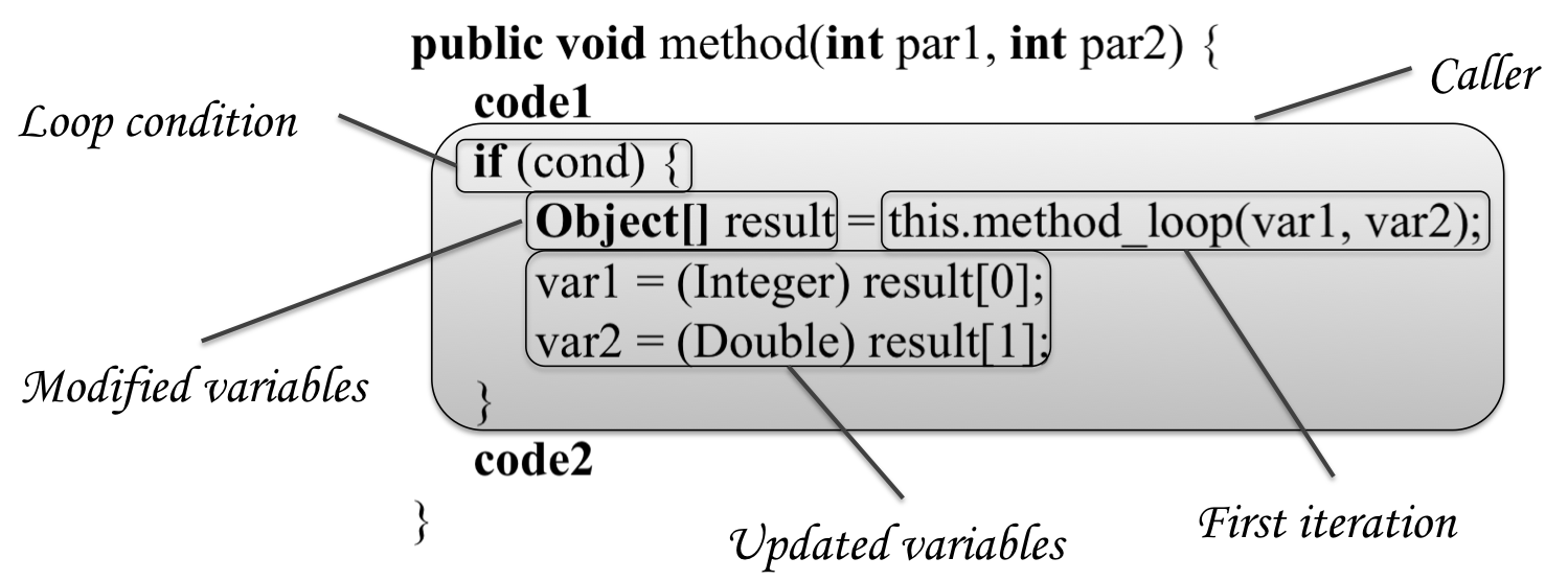
(b) Transformed method

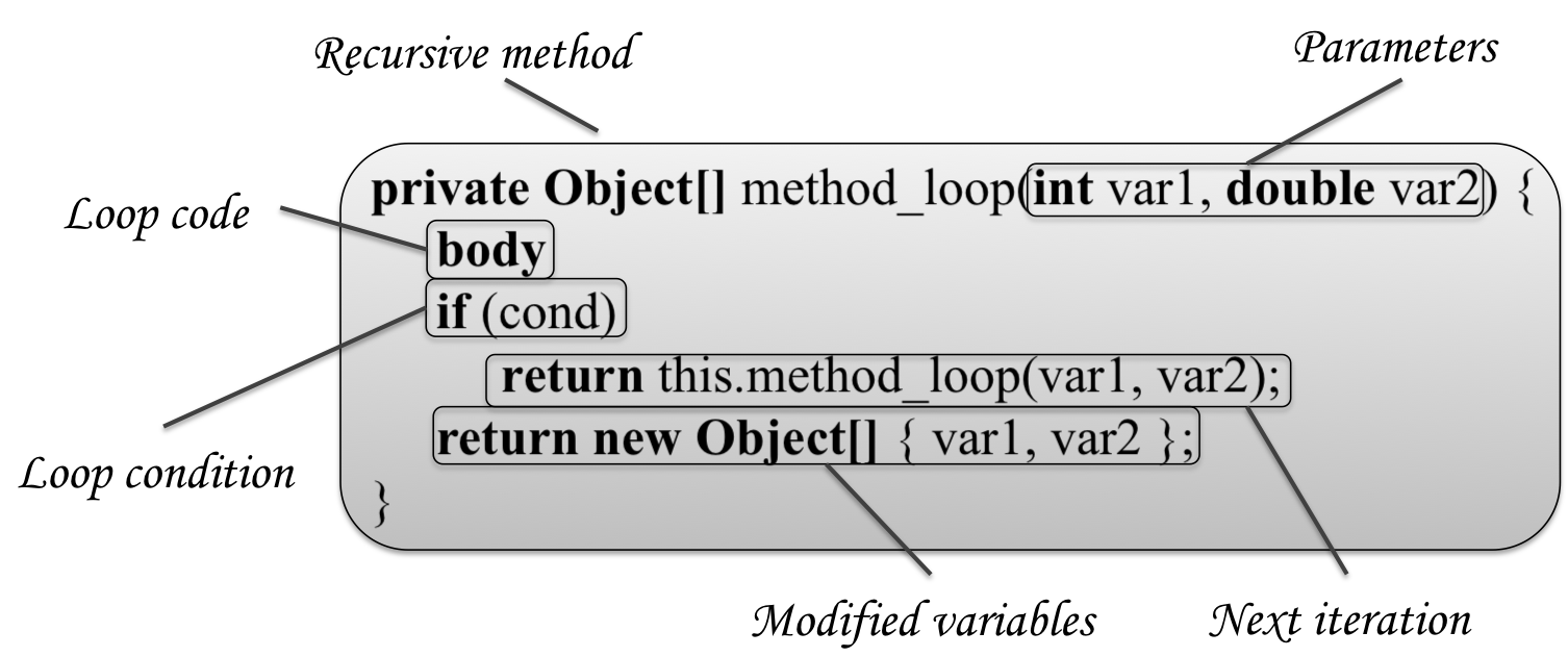
(c) Recursive method

Figure 1: while-loop transformation

In Table 2 we show a general overview of the steps needed to transform a Java iterative while-loop into an equivalent recursive method. Each step is described in the following.

Step	Correspondence with Figure 1
	Figure 1(b)
1)    Substitute the loop by a call to the recursive method	Caller
1.1)      If the loop condition is satisfied	Loop condition
1.1.1)        Perform the first iteration	First iteration
1.2)      Catch the variables modified during the recursion	Modified variables
1.3)      Update the modified variables	Updated variables
	Figure 1(c)
2)    Create the recursive method	Recursive method
2.1)      Define the method’s parameters	Parameters
2.2)      Define the code of the recursive method
2.2.1)        Include the code of the original loop	Loop code
2.2.2)        If the loop condition is satisfied	Loop condition
2.2.2.1)          Perform the next iteration	Next iteration
2.2.3)        Otherwise return the modified variables	Modified variables

Table 2: Steps of the while-loop transformation

2.1.1 Substitute the loop by a call to the recursive method

The first step is to remove the original loop and substitute it with a call to the new recursive method. We can see this substitution in Figure 1(b). Observe that some parts of the transformation have been labeled to ease later references to the code. The tasks performed during the substitution are explained in the following:

• Perform the first iteration
  In the while-loop, first of all we check whether the loop condition holds. If it does not hold, then the loop is not executed. Otherwise, the first iteration is performed by calling the recursive method with the variables used inside the loop as arguments of the method call. Hence, we need an analysis to know what variables are used inside the loop. The recursive method is in charge of executing as many iterations of the loop as needed.

• Catch the variables modified during the recursion
  The variables modified during the recursion cannot be automatically updated in Java because all parameters are passed by value. Therefore, if we modify an argument inside a method we are only modifying a copy of the original variable. This also happens with objects. Hence, in order to output those modified variables that are needed outside the loop, we use an array of objects. Because the modified variables can be of any data type, we use an array of objects of class Object.

  In presence of call-by-reference, this step should be omitted.

• Update the modified variables
  After the execution of the loop, the modified variables are returned inside an Object array. Each variable in this array must be cast to its respective type before being assigned to the corresponding variable declared before the loop.

  In presence of call-by-reference, this step should be omitted.

2.1.2 Create the recursive method

Once we have substituted the loop, we create a new method that implements the loop in a recursive way. This recursive method is shown in Figure 1(c).

The code of the recursive method is explained in the following:

• Define the method’s parameters
  There are variables declared inside a method but declared outside the loop and used by this loop. When the loop is transformed into a recursive method, these variables are not accessible from inside the recursive method. Therefore, they must be passed as arguments in the calls to it. Hence, the parameters of the recursive method are the intersection between the variables declared before the loop and the variables used inside it.

• Define the code of the recursive method
  Each iteration of the original iterative loop is emulated with a call to the new recursive method. Therefore in the code of the recursive method we have to execute the current iteration and control whether the next iteration must be executed or not.

  • Include the code of the original loop
    When the recursive method is invoked it means that we want to execute one iteration of the loop. Therefore, we place the original code of the loop at the beginning of the recursive method. This code is supposed to update the variables that control the loop condition. Otherwise, the original loop is in fact an infinite loop and the recursive method created will be invoked infinitely.

  • Perform the next iteration
    Once the iteration is executed, we check the loop condition again to know whether another iteration must still be executed. In such a case, we perform the next iteration with the same arguments. Note that the values of the arguments can be modified during the execution of the iteration, therefore, each iteration has different arguments values, but the names and the number of arguments remain always the same.

  • Otherwise return the modified variables
    If the loop condition does not hold, the loop ends and thus we must finish the sequence of recursive method calls and return to the original method in order to continue executing the rest of the code. Because the arguments have been updated in each recursive call, at this point we have the last values of the variables involved in the loop. Hence these variables must be returned in order to update them in the original method. Observe that these variables are passed from iteration to iteration during the execution of the recursive method until it is finally returned to the recursive method caller.

    In presence of call-by-reference, this step should be omitted.

Figure 2 shows an example of transformation of a while-loop.

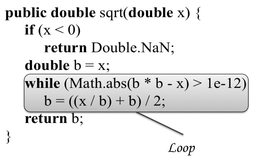
(a) Original method

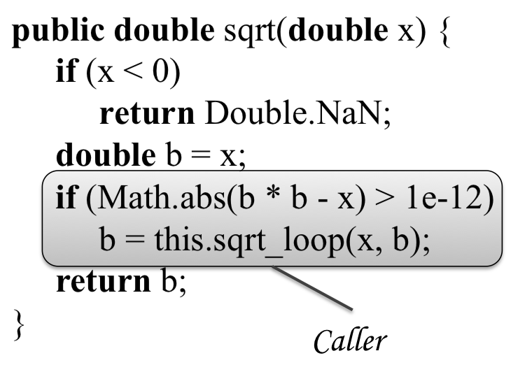
(b) Transformed method

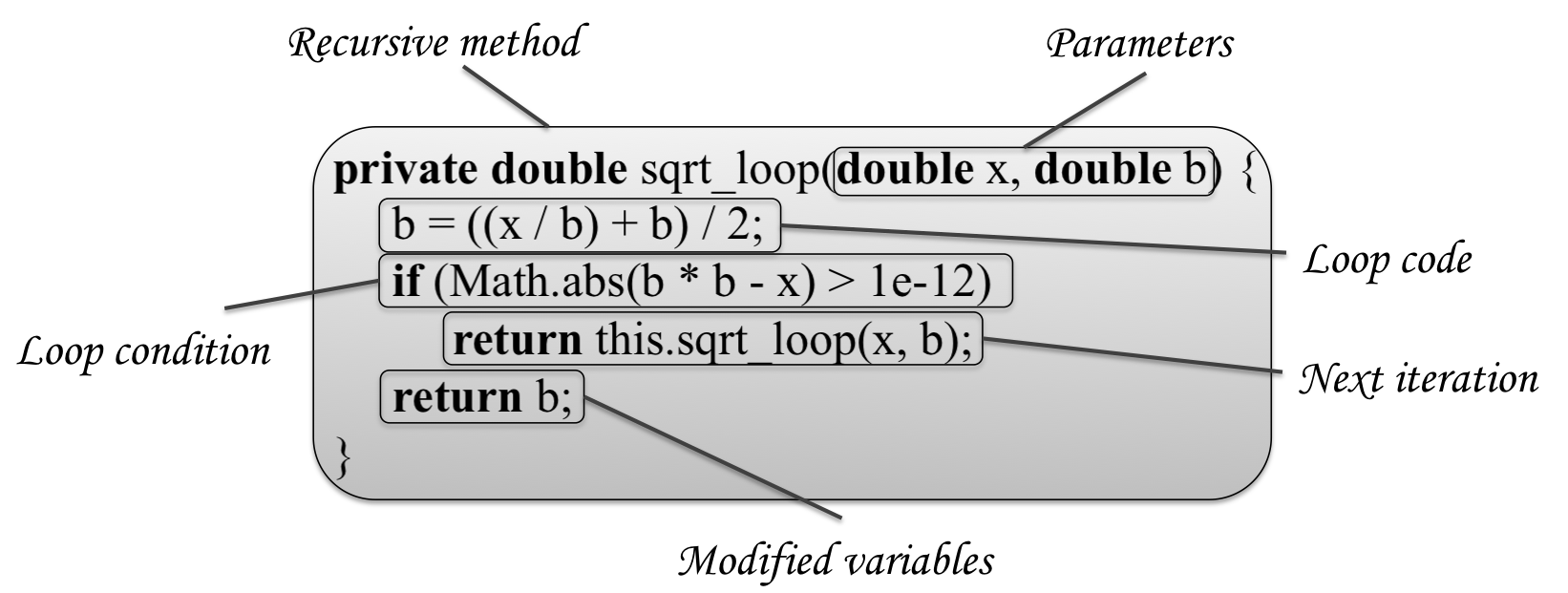
(c) Recursive method

Figure 2: while-loop transformation

2.2 Transformation of do-loops

do-loops behave exactly in the same way as while-loops except in one detail: The first iteration of the do-loop is always performed. In Figure 3 we can see an example of a do-loop.

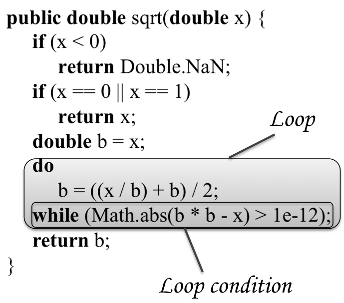
Figure 3: do-loop

This code obtains the square root value of variable x as the code in Algorithm 1. The difference is that, if variable x is either 0 or 1, then the method directly returns variable x, otherwise the loop is performed in order to calculate the square root. In order to transform the do-loop into a recursive method, we can follow the same steps used in Table 2 with only one change: in step 1.1 the loop condition is not evaluated; instead, we only need to add a new code block to ensure that those variables created during the transformation are not available outside the transformed code.

Figure 4 illustrates the only change needed to transform the do-loop into a recursive method. Observe that in this example there is no need to introduce a new block, because the transformed code does not create new variables, but in the general case the block could be needed.

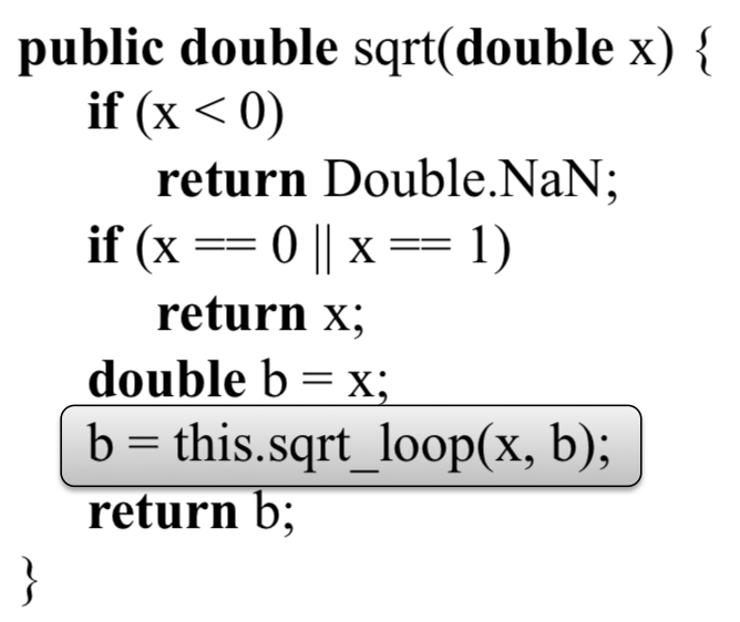
(a) Recursive method caller

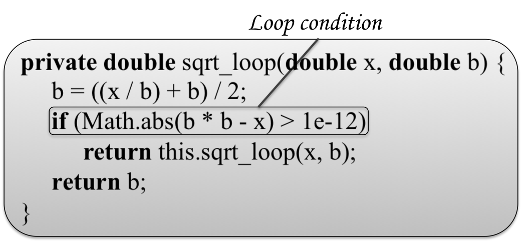
(b) Recursive method

Figure 4: do-loop transformation

• Add a new code block
  Observe in Table 1, in column Caller, that, contrarily to while-loops, do-loops need to introduce a new block (i.e., a new scope). The reason is that there could exist variables with the same name as the variables created during the transformation (e.g., result). Hence, the new block avoids variable clashes and limits the scope of the variables created by the transformation.

2.3 Transformation of for-loops

One of the most frequently used loops in Java is the for-loop. This loop behaves exactly in the same way as the while-loop except in one detail: for-loops provide the programmer with a mechanism to declare, initialize and update variables that will be accessible inside the loop.

In Figure 5(a) we can see an example of a for-loop. This code obtains the square root value of variable x exactly as the code in Algorithm 1, but it also prints the approximation obtained in every iteration. We can see in Figure 5(b) and 5(c) the additional changes needed to transform the for-loop into a recursive method.

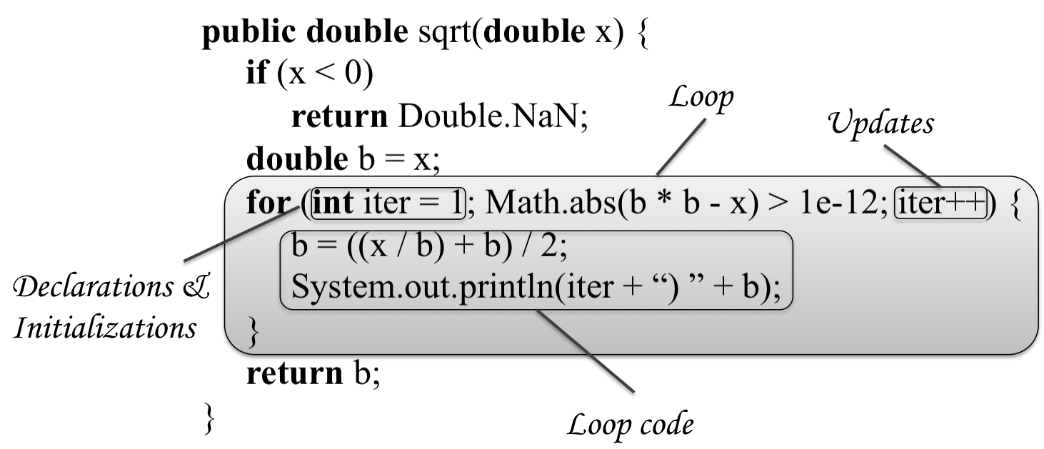
(a) For loop

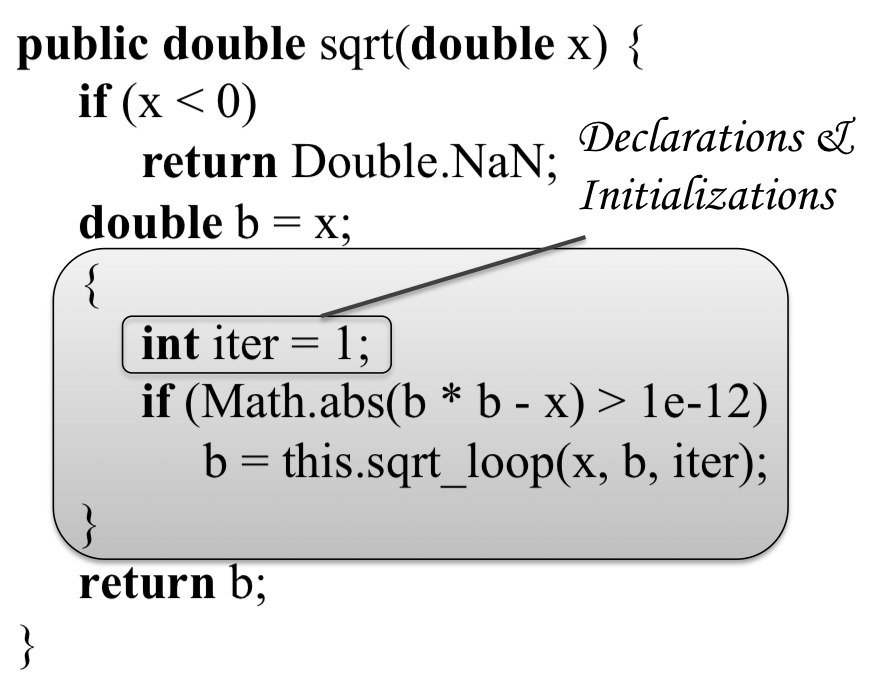
(b) Recursive method caller

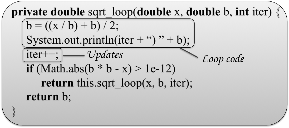
(c) Recursive method

Figure 5: for-loop transformation

As shown in Figure 5, in order to transform the for-loop into a recursive method, we can follow the same steps used in Table 2, but we have to make three changes:

• Add a new code block
  Exactly in the same way and with the same purpose as in do-loops.

• Add the declarations/initializations at the beginning of the block
  In the original method, those variables created during the declaration and initialization of the loop are only available inside it (and not in the code that follows the loop). We must ensure that these variables keep the same scope in the transformed code. This can be easily achieved with the new block. In the transformed code, those variables are declared and initialized at the beginning of the new block, and they are passed as arguments to the recursive method in every iteration to make them accessible inside it.

• Add the updates between the loop code and the loop condition
  In for-loops there exists the possibility of executing code between iterations. This code is usually a collection of updates of the variables declared at the beginning of the loop (e.g., in Figure 5(a) this code is iter++). However, this code could be formed by a series of expressions separated by commas that could include method invocations, assignments, etc. Because this update code is always executed before the condition of the loop, it must be placed in the recursive method between the loop code and the loop condition.

2.4 Transformation of foreach-loops

foreach-loops are specially useful to traverse collections of elements. In particular, this kind of loops traverses a given collection and it executes a block of code for each element. The transformation of a foreach-loop into a recursive method is different depending on the kind of collection that is traversed. In Java we can use foreach-loops either with arrays or iterable objects. We explain each transformation separately.

2.4.1 foreach-loop used to traverse arrays

An array is a composite data structure where elements have been sequentialized, and thus, they can be traversed linearly. We can see an example of a foreach-loop that traverses an array in Algorithm 3.

Algorithm 3 foreach-loop that traverses an array (iterative version)

1:  public void foreachArray() {

2:      double[] numbers = new double[] { 4.0, 9.0 };

3:      for (double number : numbers) {

4:          double sqrt = this.sqrt(number);

5:          System.out.println(“sqrt(” + number + “) = ” + sqrt);

6:      }

7:  }

This code computes and prints the square root of all elements in the array [4.0, 9.0]. Each individual square root is computed with Algorithm 1. The foreach-loop traverses the array sequentially starting in position numbers[0] until the last element in the array. The transformation of this loop into an equivalent recursive method is very similar to the transformation of a for-loop. However there are differences. For instance, foreach-loops lack of a counter. This can be observed in Figure 6 that implements a recursive method equivalent to the loop in Algorithm 3.

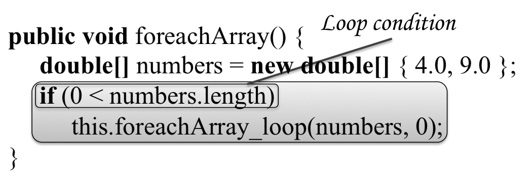
(a) Recursive method caller

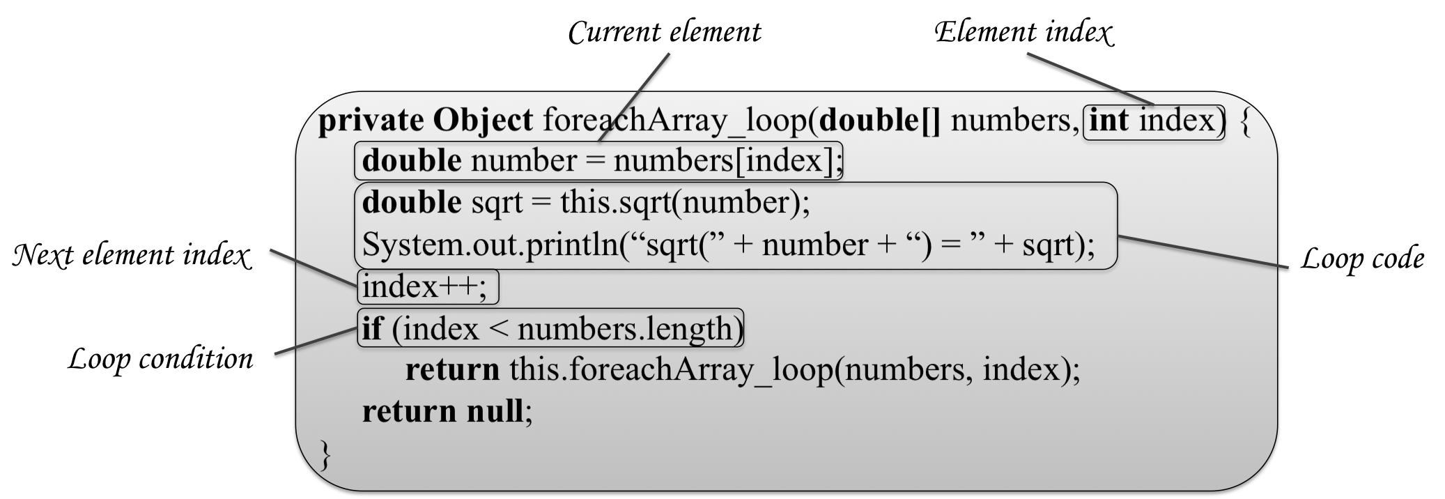
(b) Recursive method

Figure 6: foreach-loop transformation (Array version)

In Figure 6 we can see the symmetry with respect to the for-loop transformation. The only difference is the creation of a fresh variable that is passed as argument in the recursive method calls (in the example this variable is called index). This variable is used for:

• Controlling whether there are more elements to be treated
  A foreach-loop is only executed if the array contains elements. Therefore we need a loop condition in the recursive method caller and another in the recursive method to know when there are no more elements in the array and thus finish the traversal. The later is controlled with a variable (index in the example) acting as a counter.

• Obtaining the next element to be treated
  During each iteration of the foreach-loop a variable called number is instantiated with one element of the array (line 3 of Algorithm 3). In the transformation this behavior is emulated by declaring and initializing this variable at the beginning of the recursive method. It is initialized to the corresponding element of the array by using variable index.

2.4.2 foreach-loop used to traverse iterable objects

A foreach-loop can be used to traverse objects that implement the interface Iterable. Algorithm 4 shows an example of a foreach-loop using one of these objects.

Algorithm 4 foreach-loop used to traverse an iterable object (iterative version)

1:  public void foreachIterable() {

2:      List$<$Double$>$ numbers = Arrays.asList(4.0, 9.0);

3:      for (double number : numbers) {

4:          double sqrt = this.sqrt(number);

5:          System.out.println(“sqrt(” + number + “) = ” + sqrt);

6:      }

7:  }

This code behaves exactly in the same way as Algorithm 3 but using an iterable object instead of an array (numbers is an iterable object because it is an instance of class List that in turn implements the interface Iterable). The interface Iterable only has one method, called iterator, that returns an object that implements the Iterator interface. With regard to the interface Iterator, it forces the programmer to implement the next, hasNext and remove methods; and these methods allow the programmer to freely implement how the collection is traversed (e.g., the order, whether repetitions are taken into account or not, etc.). Therefore, the transformed code should use these methods to traverse the collection. We can see in Figure 7 a recursive method equivalent to Algorithm 4.

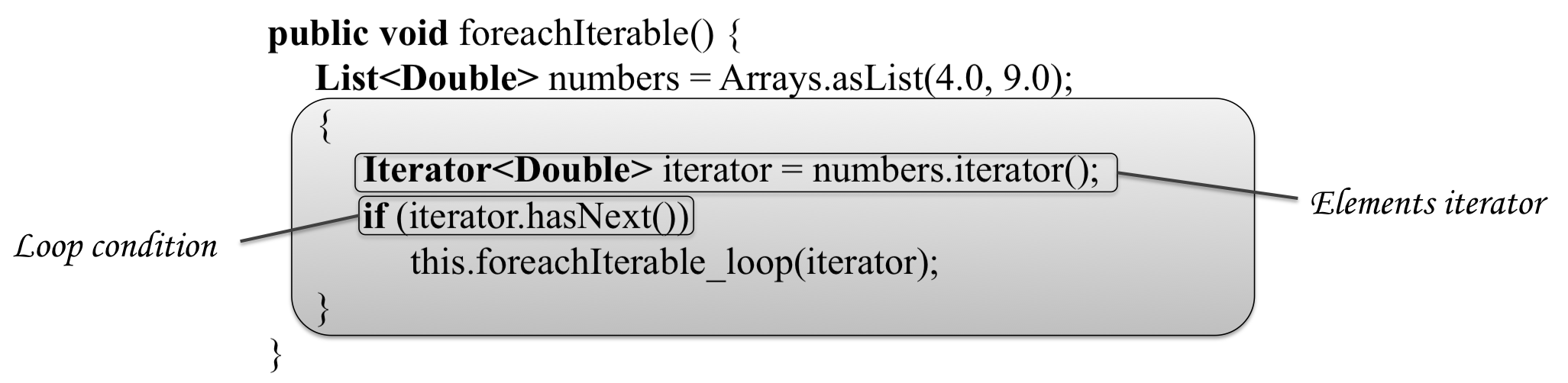
(a) Recursive method caller

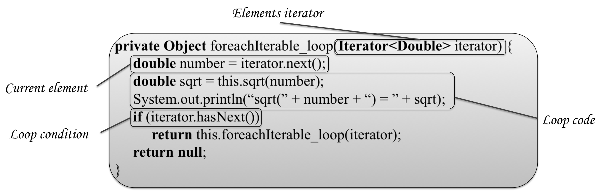
(b) Recursive method

Figure 7: foreach-loop transformation (Iterable version)

Observe that the transformed code in Figure 7 is very similar to the one in Figure 6. The only difference is the use of an iterator variable (instead of an integer variable) that controls the element of the collection to be treated. Note that method next of variable iterator allows us to know what is the next element to be treated, and method hasNext tell us whether there exist more elements to be processed yet.

3 Correctness

In this section we provide a formal semantics-based specification of our transformation in order to prove its correctness. For this, we provide a BNF syntax specification and an operational semantics of Java. We consider the subset of Java that is needed to implement the transformation (if-then-else, while, method calls, return, etc.), and we ignore the rest of syntax elements for the sake of simplicity (they do not have any influence because any command inside the body of the loop remains unchanged in the transformed code). Moreover, in this section, we center the discussion on while-loops and prove properties for this kind of loop. The proof for the other kinds of loops is omitted, but it would be in all cases analogous or slightly incremental.

We start with a BNF syntax of Java:

 

$$\begin{array}[]{lcl@{~~~~}l@{~~~}l}P&::=&M_1,\ldots,M_n,S_p\hfil~{}~{}~{}~{}&\mbox{ (program) }\hfil~{}~{}~{}&Domains\\ &&\hfil~{}~{}~{}~{}&\hfil~{}~{}~{}&x,y,z\ldots\in\mathbb{V}~{}\mbox{\sf(variables)}\\ &&\hfil~{}~{}~{}~{}&\hfil~{}~{}~{}&a,b,c\ldots\in\mathbb{C}~{}\mbox{\sf(constants)}\\ M&::=&m(x_1,\dots,x_n)~{}\{~{}S_p;~{}S_r~{}\}\hfil~{}~{}~{}~{}&\mbox{ (method definition) }\hfil~{}~{}~{}&$where $x_1,\ldots,x_n\in\mathbb{V}$ $\\ &&\hfil~{}~{}~{}~{}&\hfil~{}~{}~{}&$and $m$ is the name$\\ &&\hfil~{}~{}~{}~{}&\hfil~{}~{}~{}&$of the method$\\ S_p&::=&x:=E\hfil~{}~{}~{}~{}&\mbox{ (assignment) }\hfil~{}~{}~{}\\ &|&x:=m(E_0,\dots,E_n)\hfil~{}~{}~{}~{}&\mbox{ (method invocation) }\hfil~{}~{}~{}\\ &|&$if $E_b$ then $S_p\hfil~{}~{}~{}~{}&\mbox{ (if-then) }\hfil~{}~{}~{}\\ &|&$if $E_b$ then $S_p$ else $S_p\hfil~{}~{}~{}~{}&\mbox{ (if-then-else) }\hfil~{}~{}~{}\\ &|&$while $E_b$ do $S_p\hfil~{}~{}~{}~{}&\mbox{ (while) }\hfil~{}~{}~{}\\ &|&S_p;~{}S^{\prime}_p\hfil~{}~{}~{}~{}&\mbox{ (sequence) }\hfil~{}~{}~{}\\ S_r&::=&$return $E\hfil~{}~{}~{}~{}&\mbox{ (return) }\hfil~{}~{}~{}\\ E&::=&E_a\mid E_b\hfil~{}~{}~{}~{}&\mbox{ (expresion) }\hfil~{}~{}~{}\\ E_a&::=&E_a+E_a\mid E_a-E_a\mid V\hfil~{}~{}~{}~{}&\mbox{ (arithmetic expresion) }\hfil~{}~{}~{}\\ E_b&::=&E_b$ != $E_b\mid E_b==E_b\mid V\hfil~{}~{}~{}~{}&\mbox{ (boolean expresion) }\hfil~{}~{}~{}\\ V&::=&x\mid a\hfil~{}~{}~{}~{}&\mbox{ (variables or constants) }\hfil~{}~{}~{}\\ \end{array}$$

 

A program is a set of method definitions and at least one initial statement (usually a method invocation). Each method definition is composed of a set of statements followed by a return statement. For simplicity, the arguments of a method invocation can only be expressions (not statements). This is not a restriction, because any statement can be assigned to a variable and then be passed as argument of the method invocation. However, this simplification allows us to ease the semantics of method invocations and, thus, it increases readability.

In the following we consider two versions of the same program shown in Algorithms 5 and 6. We assume that in Algorithm 5 there exists a variable $x$ already defined before the loop and, for the sake of simplicity, it is the only variable modified inside $S$. Therefore, Algorithm 6 is the recursive version of the while-loop in Algorithm 5 according to our transformation, and hence, $p_0,\dots,p_n$ represent all variables defined before the loop and used in $S$ (the loop statements) and $cond$ (the loop condition). In the case that more than one variable are modified, then the output would be an array with all variables modified. We avoid this case because it is not necessary for the proof.

Algorithm 5 While version

1:  $~{}{\bf while}$ $cond$ ${\bf do}$

2:  $~{}~{}~{}~{}~{}S;$

Algorithm 6 Recursive version

1:  $~{}m(p_0,\dots,p_n)$ $\{$

2:  $~{}~{}~{}~{}~{}S;$

3:  $~{}~{}~{}~{}~{}{\bf if}$ $cond$ ${\bf then}$

4:  $~{}~{}~{}~{}~{}~{}~{}~{}~{}x:=m(a_0,\dots,a_n);$

5:  $~{}~{}~{}~{}~{}{\bf return}$ $x;$

6:  $~{}\}$

7:  $~{}{\bf if}$ $cond$ ${\bf then}$

8:  $~{}~{}~{}~{}~{}x:=m(a_0,\dots,a_n);$

In order to provide an operational semantics for this Java subset, which allows recursion, we need a stack to push and pop different frames that represent individual method activations. Frames, $f_0,f_1,\ldots\in\mathbb{F}$, are sequences of pairs variable-value. States, $s_0,s_1,\ldots\in\mathbb{S}$, are sequences of frames ($\mathbb{S}:~{}\mathbb{F}$ x $\dots$ x $\mathbb{F}$). We make the program explicitly accessible to the semantics through the use of an environment, $e\in\mathbb{E}$, represented with a sequence of functions from method names $\mathbb{M}$ to pairs of parameters $\mathbb{P}$ and statements $\mathbb{I}$ ($\mathbb{E}:~{}(\mathbb{M}\rightarrow(\mathbb{P}$ x $\mathbb{I}))$ x $\dots$ x $(\mathbb{M}\rightarrow(\mathbb{P}$ x $\mathbb{I}))$). Our semantics is based on the Java semantics described in [11] with some minor modifications. It uses a set of functions to update the state, the environment, etc.

Function $\mathit{Upd_v}$ is used to update a variable ($var$) in the current frame of the state ($s$) with a value ($value$). The current frame in the state is always the last frame introduced (i.e., the last element in the sequence of frames that represent the state). We use the standard notation $f[var\rightarrow value]$ to denote that variable $var$ in frame $f$ is updated to value $value$.

$\mathit{Upd_v}(s,~{}var\rightarrow value)=\left\{\begin{array}[]{lll}&error&\mathit{if}~{}s=[]\\ &[f_0,\dots,f_n[var\rightarrow value]]&\mathit{if}~{}s=[f_0,\dots,f_n]\\ \end{array}\right.$

Function $\mathit{Upd_r}$ records the returned value ($value$) of the current frame of the state ($s$) inside a fresh variable $\Re$ of this frame, so that other frames can consult the value returned by the current frame.

$\mathit{Upd_r}(s,~{}value)=\left\{\begin{array}[]{lll}&error&\mathit{if}~{}s=[]\\ &[f_0,\dots,f_n[\Re\rightarrow value]]&\mathit{if}~{}s=[f_0,\dots,f_n]\\ \end{array}\right.$

Function $\mathit{Upd_{vr}}$ is used to update a variable ($var$) in the penultimate frame of the state ($s$) taking the value returned by the last frame in the state (which must be previously stored in $\Re$). This happens when a method calls another method and the latter finishes returning a value. In this situation, the last frame in the state should be removed and the value returned should be updated in the penultimate frame. We use the notation $f_n(\Re)$ to consult the value of variable $\Re$ in frame $f_n$.

$\mathit{Upd_{vr}}(s,~{}var)=\left\{\begin{array}[]{lll}&error&\mathit{if}~{}s=[]~{}\mathit{or}~{}s=[f]\\ &[f_0,\dots,f_{n-1}[var\rightarrow f_n(\Re)],f_n]&\mathit{if}~{}s=[f_0,\dots,f_{n-1},f_n]\\ \end{array}\right.$

Function $\mathit{Upd_e}$ is used to update the environment ($env$) with a new method definition ($m\rightarrow(P,I)$). The environment is used in method invocations to know the method that should be executed.

$\mathit{Upd_e}(env,~{}m\rightarrow(P,I))=env[m\rightarrow(P,I)]$

Function $\mathit{AddFrame}$ adds a new frame to the state ($s$). This frame is a sequence of mappings from parameters ($p_0,\dots,p_n$) to the evaluation of arguments ($a_0,\dots,a_n$). To evaluate an expression we use function $\mathit{Eval}$: a variable is consulted in the state, a constant is just returned, and a mathematical or boolean expression is evaluated with the standard semantics. We use this notation because the evaluation of expressions does not have influence in our proofs, but it significantly reduces the size of derivations, thus, improving clarity of presentation.

$\mathit{AddFrame}(s,[p_0,\dots,p_n],[a_0,\dots,a_n])=\\ ~{}~{}~{}~{}~{}~{}~{}~{}~{}~{}~{}~{}~{}~{}~{}~{}~{}~{}~{}~{}~{}~{}~{}~{}~{}~{}~{}\left\{\begin{array}[]{lll}&[[p_0\rightarrow Eval(a_0),\dots,p_n\rightarrow Eval(a_n)]]&if~{}s=[]\\ &[f_0,\dots,f_m,[p_0\rightarrow Eval(a_0),\dots,p_n\rightarrow Eval(a_n)]]&if~{}s=[f_0,\dots,f_m]\\ \end{array}\right.$

Analogously, function $\mathit{RemFrame}$ removes the last frame inserted into the state ($s$).

$RemFrame(s)=\left\{\begin{array}[]{lll}&error&if~{}s=[]\\ &[]&if~{}s=[f]\\ &[f_0,\dots,f_n]&if~{}s=[f_0,\dots,f_n,f_{n+1}]\\ \end{array}\right.$

We are now in a position ready to introduce our Java operational semantics. Essentially, the semantics is a big-step semantics composed of a set of rules of the form: $\frac{p_1\dots p_n}{\mathit{env}~{}\vdash~{}<st,~{}s>~{}\Downarrow~{}s^{\prime}}$ that should be read as “The execution of statement $st$ in state $s$ under the environment $env$ can be reduced to state $s^{\prime}$ provided that premises $p_1\dots p_n$ hold”. The rules of the semantics are shown in Figure 8.

$\begin{array}[]{|c|}\hline\cr\\ \mathit{New~{}method}\\ \frac{\mathit{env^{\prime}}~{}=~{}\mathit{Upd_e}(env,~{}m_0~{}\rightarrow~{}(P,~{}I))~{}\land~{}\mathit{env^{\prime}}~{}\vdash~{}<m_1~{}i,~{}s>~{}\Downarrow~{}s^{\prime}~{}}{\mathit{env}~{}\vdash~{}<m_0(P)\{I\}~{}m_1~{}i,~{}s>~{}\Downarrow~{}s^{\prime}}\\ \\ \mathit{Empty~{}statement}\\ \frac{}{\mathit{env}~{}\vdash~{}<\surd,~{}s>~{}\Downarrow~{}s}\\ \\ \mathit{Asignment}\\ \frac{s^{\prime}~{}=~{}\mathit{Upd_v}(s,~{}x~{}\rightarrow~{}\mathit{Eval}(op,~{}s))}{\mathit{env}~{}\vdash~{}<x:=op,~{}s>~{}\Downarrow~{}s^{\prime}}\\ \\ \mathit{Method~{}invocation}\\ \frac{(P,~{}I)~{}=~{}\mathit{env}(m)~{}\land~{}s^{\prime}~{}=~{}\mathit{AddFrame}(s,P,A)~{}\land~{}\mathit{env}~{}\vdash~{}<I,~{}s^{\prime}>~{}\Downarrow~{}s^{\prime\prime}~{}\land~{}s^{\prime\prime\prime}~{}=~{}\mathit{Upd_{vr}}(s^{\prime\prime},x)~{}\land~{}s^{\prime\prime\prime\prime}~{}=~{}\mathit{RemFrame}(s^{\prime\prime\prime})}{\mathit{env}~{}\vdash~{}<x:=m(A),~{}s>~{}\Downarrow~{}s^{\prime\prime\prime\prime}}\\ \\ \mathit{If}\\ \begin{array}[]{c}\frac{\mathit{env}~{}\vdash~{}<if~{}cond~{}then~{}i_0~{}else~{}\surd,~{}s>~{}\Downarrow~{}s^{\prime}}{\mathit{env}~{}\vdash~{}<if~{}cond~{}then~{}i_0,~{}s>~{}\Downarrow~{}s^{\prime}}\\ \\ \frac{<cond,~{}s>~{}\Rightarrow~{}true~{}\land~{}\mathit{env}~{}\vdash~{}<i_0,~{}s>~{}\Downarrow~{}s^{\prime}}{\mathit{env}~{}\vdash~{}<if~{}cond~{}then~{}i_0~{}else~{}i_1,~{}s>~{}\Downarrow~{}s^{\prime}}\\ \\ \frac{<cond,~{}s>~{}\Rightarrow~{}false~{}\land~{}\mathit{env}~{}\vdash~{}<i_1,~{}s>~{}\Downarrow~{}s^{\prime}}{\mathit{env}~{}\vdash~{}<if~{}cond~{}then~{}i_0~{}else~{}i_1,~{}s>~{}\Downarrow~{}s^{\prime}}\\ \end{array}\\ \\ \mathit{While}\\ \begin{array}[]{c}\frac{<cond,~{}s>~{}\Rightarrow~{}false}{\mathit{env}~{}\vdash~{}<while~{}cond~{}do~{}i,~{}s>~{}\Downarrow~{}s}\\ \\ \frac{<cond,~{}s>~{}\Rightarrow~{}true~{}\land~{}\mathit{env}~{}\vdash~{}<i,~{}s>~{}\Downarrow~{}s^{\prime}~{}\land~{}\mathit{env}~{}\vdash~{}<while~{}cond~{}do~{}i,~{}s^{\prime}>~{}\Downarrow~{}s^{\prime\prime}}{\mathit{env}~{}\vdash~{}<while~{}cond~{}do~{}i,~{}s>~{}\Downarrow~{}s^{\prime\prime}}\\ \end{array}\\ \\ \mathit{Sequence}\\ \frac{\mathit{env}~{}\vdash~{}<i_0,~{}s>~{}\Downarrow~{}s^{\prime}~{}\land~{}\mathit{env}~{}\vdash~{}<i_1,~{}s^{\prime}>~{}\Downarrow~{}s^{\prime\prime}}{\mathit{env}~{}\vdash~{}<i_0;~{}i_1,~{}s>~{}\Downarrow~{}s^{\prime\prime}}\\ \\ \mathit{Return}\\ \frac{s^{\prime}~{}=~{}\mathit{Upd_r}(s,~{}\mathit{Eval}(op,~{}s))}{\mathit{env}~{}\vdash~{}<\mathit{return}~{}op,~{}s>~{}\Downarrow~{}s^{\prime}}\\ \\ \hline\cr\end{array}$

Figure 8: Java Semantics

We can now prove our main result.

Theorem 3.1 (Correctness)

Algorithm 6 is semantically equivalent to Algorithm 5.

Proof

We prove this claim by showing that the final state of Algorithm 5 is always the same as the final state of Algorithm 6. The semantics of a program $P$ is:

$S(P)=s~{}~{}$ iff $~{}~{}\mathit{[]}\vdash<P,~{}[]>\Downarrow s$

Therefore, we say that two programs $P_1$ and $P_2$ are equivalent if they have the same semantics:

$S(P_1)=S(P_2)~{}~{}$ iff $~{}~{}\mathit{[]}\vdash<P_1,~{}[]>\Downarrow s_1~{}~{}\land~{}~{}\mathit{[]}\vdash<P_2,~{}[]>\Downarrow s_2~{}~{}\land~{}~{}s_1=s_2$

For the sake of generality, in the following we consider that the loops can appear inside any other code. Therefore, the environment and the state are not necessarily empty. Thus, we will assume an initial environment $env_0$ and an initial state $s$: $\mathit{env_0}\vdash<P,~{}s>$. We proof this semantic equivalence analyzing two possible cases depending on whether the loop is executed or not.

1) Zero iterations
This situation can only happen when the condition $cond$ is not satisfied the first time it is evaluated. Hence, we have the following semantics derivation for each program:

Iterative version

$\mathit{env}_0~{}\vdash~{}<while~{}cond~{}do~{}S,~{}s>~{}\Downarrow~{}s<cond,~{}s>~{}\Rightarrow~{}false$

Recursive version

$\mathit{env}_0~{}\vdash~{}<m(P)~{}\{~{}S;I~{}\}~{}if~{}cond~{}then~{}t,~{}s>~{}\Downarrow~{}s\lx@proof@logical@and\mathit{env}=\mathit{Upd_e}(\mathit{env}_0,~{}m~{}\rightarrow~{}(P,~{}S;I))\mathit{env}~{}\vdash~{}<if~{}cond~{}then~{}t,~{}s>~{}\Downarrow~{}s\mathit{env}~{}\vdash~{}<if~{}cond~{}then~{}t~{}else~{}\surd,~{}s>~{}\Downarrow~{}s\lx@proof@logical@and<cond,~{}s>~{}\Rightarrow~{}false\mathit{env}~{}\vdash~{}<\surd,~{}s>~{}\Downarrow~{}s$

Clearly, the state is never modified neither in the iterative version nor in the recursive version. Therefore, both versions are semantically equivalent.

2) One or more iterations
This means that the condition $cond$ is satisfied at least once. Let us consider that $cond$ is satisfied $n$ times, producing $n$ iterations. We proof that the final state of the program in Algorithm 6 is equal to the final state of the program in Algorithm 5 by induction over the number of iterations performed.

(Base Case) In the base case, only one iteration is executed. Hence, we have the following derivations:

Iterative version

$\mathit{env}_0~{}\vdash~{}<while~{}cond~{}do~{}S,~{}s>~{}\Downarrow~{}s^{1}\lx@proof@logical@and<cond,~{}s>~{}\Rightarrow~{}true\mathit{env}_0~{}\vdash~{}<S,~{}s>~{}\Downarrow~{}s^{1}\mathit{env}_0~{}\vdash~{}<while~{}cond~{}do~{}S,~{}s^{1}>~{}\Downarrow~{}s^{1}<cond,~{}s>~{}\Rightarrow~{}false$

Recursive version

$\bigtriangleup\mathit{env}~{}\vdash~{}<S;I,~{}s^{1}>~{}\Downarrow~{}s^{3}\lx@proof@logical@and\mathit{env}~{}\vdash~{}<S,~{}s^{1}>~{}\Downarrow~{}s^{2}\mathit{env}~{}\vdash~{}<if~{}cond~{}then~{}t;~{}return~{}x,~{}s^{2}>~{}\Downarrow~{}s^{3}\lx@proof@logical@and\mathit{env}~{}\vdash~{}<if~{}cond~{}then~{}t,~{}s^{2}>~{}\Downarrow~{}s^{2}\mathit{env}~{}\vdash~{}<if~{}cond~{}then~{}t~{}else~{}\surd,~{}s^{2}>~{}\Downarrow~{}s^{2}\lx@proof@logical@and<cond,~{}s^{2}>~{}\Rightarrow~{}false\mathit{env}~{}\vdash~{}<\surd,~{}s^{2}>~{}\Downarrow~{}s^{2}\mathit{env}~{}\vdash~{}<return~{}x,~{}s^{2}>~{}\Downarrow~{}s^{3}s^{3}~{}=~{}\mathit{Upd_r}(s^{2},~{}\mathit{Eval}(x,s^{2}))$

$\mathit{env}~{}\vdash~{}<if~{}cond~{}then~{}t,~{}s>~{}\Downarrow~{}s^{5}\mathit{env}~{}\vdash~{}<if~{}cond~{}then~{}t~{}else~{}\surd,~{}s>~{}\Downarrow~{}s^{5}\lx@proof@logical@and<cond,~{}s>~{}\Rightarrow~{}true\mathit{env}~{}\vdash~{}<x:=m(a_0,\dots,a_n),~{}s>~{}\Downarrow~{}s^{5}\lx@proof@logical@and(P,I)=env(m)s^{1}~{}=~{}\mathit{AddFrame}(s,P,[a_0,\dots,a_n])\bigtriangleup s^{4}~{}=~{}\mathit{Upd_{vr}}(s^{3},x)s^{5}~{}=~{}\mathit{RemFrame}(s^{4})$

We can assume that variable $x$ has an initial value $z^{0}$, which must be the same in both versions of the algorithm. Then, states are modified during the iteration as follows:

$\begin{array}[]{lc@{~~~~~~~~~~~~~~~~~~~~~}l}$\text@underline{Iterative version}$&\hfil~{}~{}~{}~{}~{}~{}~{}~{}~{}~{}~{}~{}~{}~{}~{}~{}~{}~{}~{}~{}~{}&$\text@underline{Recursive version}$\\ s=[f_0]\Rightarrow f_0=\{x\rightarrow z^{0}\}&\hfil~{}~{}~{}~{}~{}~{}~{}~{}~{}~{}~{}~{}~{}~{}~{}~{}~{}~{}~{}~{}~{}&s=[f_0]\Rightarrow f_0=\{x\rightarrow z^{0}\}\\ s^{1}=[f_0]\Rightarrow f_0=\{x\rightarrow z^{1}\}&\hfil~{}~{}~{}~{}~{}~{}~{}~{}~{}~{}~{}~{}~{}~{}~{}~{}~{}~{}~{}~{}~{}&s^{1}=[f_0,f_1]\Rightarrow f_0=\{x\rightarrow z^{0}\}\land f_1=\{x\rightarrow z^{0}\}\\ &\hfil~{}~{}~{}~{}~{}~{}~{}~{}~{}~{}~{}~{}~{}~{}~{}~{}~{}~{}~{}~{}~{}&s^{2}=[f_0,f_1]\Rightarrow f_0=\{x\rightarrow z^{0}\}\land f_1=\{x\rightarrow z^{1}\}\\ &\hfil~{}~{}~{}~{}~{}~{}~{}~{}~{}~{}~{}~{}~{}~{}~{}~{}~{}~{}~{}~{}~{}&s^{3}=[f_0,f_1]\Rightarrow f_0=\{x\rightarrow z^{0}\}\land f_1=\{x\rightarrow z^{1},\Re\rightarrow z^{1}\}\\ &\hfil~{}~{}~{}~{}~{}~{}~{}~{}~{}~{}~{}~{}~{}~{}~{}~{}~{}~{}~{}~{}~{}&s^{4}=[f_0,f_1]\Rightarrow f_0=\{x\rightarrow z^{1}\}\land f_1=\{x\rightarrow z^{1},\Re\rightarrow z^{1}\}\\ &\hfil~{}~{}~{}~{}~{}~{}~{}~{}~{}~{}~{}~{}~{}~{}~{}~{}~{}~{}~{}~{}~{}&s^{5}=[f_0]\Rightarrow f_0=\{x\rightarrow z^{1}\}\\ \end{array}$

Clearly, with the same initial states, both algorithms produce the same final state.

(Induction Hypothesis) We assume as the induction hypothesis that executing $i$ iterations in both versions with an initial value $z^{0}$ for $x$ then, if the iterative version obtains a final value $z^{n}$ for $x$ then the recursive version correctly obtains and stores the same final value $z^{n}$ for variable $x$ in the top frame.

$\begin{array}[]{lc@{~~~~~~~~~~~~~~~~~~~~~}l}$\text@underline{Iterative version}$&\hfil~{}~{}~{}~{}~{}~{}~{}~{}~{}~{}~{}~{}~{}~{}~{}~{}~{}~{}~{}~{}~{}&$\text@underline{Recursive version}$\\ s=[f_0]\Rightarrow f_0=\{x\rightarrow z^{0}\}&\hfil~{}~{}~{}~{}~{}~{}~{}~{}~{}~{}~{}~{}~{}~{}~{}~{}~{}~{}~{}~{}~{}&s=[f_0]\Rightarrow f_0=\{x\rightarrow z^{0}\}\\ \dots&\hfil~{}~{}~{}~{}~{}~{}~{}~{}~{}~{}~{}~{}~{}~{}~{}~{}~{}~{}~{}~{}~{}&\dots\\ s^{\prime}=[f_0]\Rightarrow f_0=\{x\rightarrow z^{n}\}&\hfil~{}~{}~{}~{}~{}~{}~{}~{}~{}~{}~{}~{}~{}~{}~{}~{}~{}~{}~{}~{}~{}&\indent s^{\prime}=[f_0]\Rightarrow f_0=\{x\rightarrow z^{n}\}\\ \end{array}$

(Inductive Case) We now prove that executing $i+1$ iterations in both versions with an initial value $z^{0}$ for $x$ then, if the iterative version obtains a final value $z^{n}$ for $x$ then the recursive version correctly obtains and stores the same final value $z^{n}$ for variable $x$ in the top frame.

The derivation obtained for each version is the following:

Iterative version

$\mathit{env}_0~{}\vdash~{}<while~{}cond~{}do~{}S,~{}s>~{}\Downarrow~{}s^{2}\lx@proof@logical@and<cond,~{}s>~{}\Rightarrow~{}true\mathit{env}_0~{}\vdash~{}<S,~{}s>~{}\Downarrow~{}s^{1}\mathit{env}_0~{}\vdash~{}<while~{}cond~{}do~{}S,~{}s^{1}>~{}\Downarrow~{}s^{2}\mathit{Induction}~{}\mathit{hypotesis}$

Recursive version

$\bigtriangleup\mathit{env}~{}\vdash~{}<S;I,~{}s^{1}>~{}\Downarrow~{}s^{4}\lx@proof@logical@and\mathit{env}~{}\vdash~{}<S,~{}s^{1}>~{}\Downarrow~{}s^{2}\mathit{env}~{}\vdash~{}<if~{}cond~{}then~{}t;~{}return~{}x,~{}s^{2}>~{}\Downarrow~{}s^{4}\lx@proof@logical@and\mathit{env}~{}\vdash~{}<if~{}cond~{}then~{}t,~{}s^{2}>~{}\Downarrow~{}s^{3}\mathit{Induction}~{}\mathit{hypotesis}\mathit{env}~{}\vdash~{}<return~{}x,~{}s^{3}>~{}\Downarrow~{}s^{4}s^{4}~{}=~{}\mathit{Upd_r}(s^{3},~{}\mathit{Eval}(x,s^{3}))$

$\mathit{env}~{}\vdash~{}<if~{}cond~{}then~{}t,~{}s>~{}\Downarrow~{}s^{6}\mathit{env}~{}\vdash~{}<if~{}cond~{}then~{}t~{}else~{}\surd,~{}s>~{}\Downarrow~{}s^{6}\lx@proof@logical@and<cond,~{}s>~{}\Rightarrow~{}true\mathit{env}~{}\vdash~{}<x:=m(a_0,\dots,a_n),~{}s>~{}\Downarrow~{}s^{6}\lx@proof@logical@and(P,I)=env(m)s^{1}~{}=~{}\mathit{AddFrame}(s,P,[a_0,\dots,a_n])\bigtriangleup s^{5}~{}=~{}\mathit{Upd_{vr}}(s^{4},x)s^{6}~{}=~{}\mathit{RemFrame}(s^{5})$

Because both algorithms have the same initial value $z^{0}$ for $x$ then the states during the iteration are modified as follows (the * state is obtained by the induction hypothesis):

$\begin{array}[]{lc@{~~~~~~~~~~~~~~~~~~~~~}l}$\text@underline{Iterative version}$&\hfil~{}~{}~{}~{}~{}~{}~{}~{}~{}~{}~{}~{}~{}~{}~{}~{}~{}~{}~{}~{}~{}&$\text@underline{Recursive version}$\\ s=[f_0]\Rightarrow f_0=\{x\rightarrow z^{0}\}&\hfil~{}~{}~{}~{}~{}~{}~{}~{}~{}~{}~{}~{}~{}~{}~{}~{}~{}~{}~{}~{}~{}&s=[f_0]\Rightarrow f_0=\{x\rightarrow z^{0}\}\\ s^{1}=[f_0]\Rightarrow f_0=\{x\rightarrow z^{1}\}&\hfil~{}~{}~{}~{}~{}~{}~{}~{}~{}~{}~{}~{}~{}~{}~{}~{}~{}~{}~{}~{}~{}&s^{1}=[f_0,f_1]\Rightarrow f_0=\{x\rightarrow z^{0}\}\land f_1=\{x\rightarrow z^{0}\}\\ s^{2}=[f_0]\Rightarrow f_0=\{x\rightarrow z^{n}\}*&\hfil~{}~{}~{}~{}~{}~{}~{}~{}~{}~{}~{}~{}~{}~{}~{}~{}~{}~{}~{}~{}~{}&s^{2}=[f_0,f_1]\Rightarrow f_0=\{x\rightarrow z^{0}\}\land f_1=\{x\rightarrow z^{1}\}\\ &\hfil~{}~{}~{}~{}~{}~{}~{}~{}~{}~{}~{}~{}~{}~{}~{}~{}~{}~{}~{}~{}~{}&s^{3}=[f_0,f_1]\Rightarrow f_0=\{x\rightarrow z^{0}\}\land f_1=\{x\rightarrow z^{n}\}*\\ &\hfil~{}~{}~{}~{}~{}~{}~{}~{}~{}~{}~{}~{}~{}~{}~{}~{}~{}~{}~{}~{}~{}&s^{4}=[f_0,f_1]\Rightarrow f_0=\{x\rightarrow z^{0}\}\land f_1=\{x\rightarrow z^{n},\Re\rightarrow z^{n}\}\\ &\hfil~{}~{}~{}~{}~{}~{}~{}~{}~{}~{}~{}~{}~{}~{}~{}~{}~{}~{}~{}~{}~{}&s^{5}=[f_0,f_1]\Rightarrow f_0=\{x\rightarrow z^{n}\}\land f_1=\{x\rightarrow z^{n},\Re\rightarrow z^{n}\}\\ &\hfil~{}~{}~{}~{}~{}~{}~{}~{}~{}~{}~{}~{}~{}~{}~{}~{}~{}~{}~{}~{}~{}&s^{6}=[f_0]\Rightarrow f_0=\{x\rightarrow z^{n}\}\\ \end{array}$

Hence, Algorithm 6 and Algorithm 5 obtain the same final state, and thus, they are semantically equivalent.

4 Conclusions

Transforming loops to recursion is useful in many situations such as, e.g., debugging, verification or memory hierarchies optimization. It is therefore surprising that there did not exist an automatic transformation from loops to recursion, but it is even more surprising that no public report exists that describes how to implement this transformation.

In this article the transformation of each kind of Java loop has been described independently with a specific treatment for it that is illustrated with an example of use. Moreover, the transformation has been described in such a way that it can be easily adapted to any other language where recursion and iteration exist.

References

- [1] H. G. Baker. Garbage collection, tail recursion and first-class continuations in stack-oriented languages. Patent, dec 1996. US 5590332.
- [2] W. Clinger. Proper tail recursion and space efficiency. ACM SIGPLAN Notices, 33(5):174–185, may 1998.
- [3] E. Elmroth and F. G. Gustavson. Applying recursion to serial and parallel QR factorization leads to better performance. IBM Journal of Research and Development, 44(4):605–624, 2000.
- [4] F. G. Gustavson. Recursion leads to automatic variable blocking for dense linear-algebra algorithms. IBM Journal of Research and Development, 41(6):737–756, 1997.
- [5] C. Hanson. Efficient stack allocation for tail-recursive languages. In Proceedings of the 1990 ACM conference on LISP and Functional Programming (LFP’90), pages 106–118, New York, NY, USA, 1990. ACM.
- [6] P. G. Harrison and H. Khoshnevisan. A new approach to recursion removal. Electronic Notes in Theoretical Computer Science, 93(1):91–113, feb 1992.
- [7] D. Insa and J. Silva. An Algorithmic Debugger for Java. In Proceedings of the 26th IEEE International Conference on Software Maintenance (ICSM 2010), pages 1–6, 2010.
- [8] D. Insa, J. Silva, and C. Tomás. Enhancing Declarative Debugging with Loop Expansion and Tree Compression. In E. Albert, editor, Proceedings of the 22th International Symposium on Logic-based Program Synthesis and Transformation (LOPSTR 2012), volume 7844 of Lecture Notes in Computer Science (LNCS), pages 71–88. Springer, sep 2012.
- [9] Y. A. Liu and S. D. Stoller. From recursion to iteration: what are the optimizations? In Proceedings of the 2000 ACM-SIGPLAN Workshop on Partial Evaluation and semantics-based Program Manipulation (PEPM’00), pages 73–82, New York, NY, USA, 2000. ACM.
- [10] J. McCarthy. Towards a Mathematical Science of Computation. In Proceedings of the 2nd International Federation for Information Processing Congress (IFIP’62), pages 21–28. North-Holland, 1962.
- [11] H. R. Nielson and F. Nielson. Semantics with Applications: A Formal Introduction. John Wiley & Sons, Inc., New York, NY, USA, 1992.
- [12] Q. Yi, V. Adve, and K. Kennedy. Transforming Loops to Recursion for Multi-level Memory Hierarchies. In Proceedings of the 21st ACM-SIGPLAN Conference on Programming Language Design and Implementation (PLDI’00), pages 169–181, 2000.