Fifty years of Hubbard and Anderson lattice models: from magnetism to unconventional superconductivity - A brief overview

Abstract

We briefly overview the importance of Hubbard and Anderson-lattice models as applied to explanation of high-temperature and heavy-fermion superconductivity. Application of the models during the last two decades provided an explanation of the paired states in correlated fermion systems and thus extended essentially their earlier usage to the description of itinerant magnetism, fluctuating valence, and the metal-insulator transition. In second part, we also present some of the new results concerning the unconventional superconductivity and obtained very recently in our group. A comparison with experiment is also discussed, but the main emphasis is put on rationalization of the superconducting properties of those materials within the real-space pairing mechanism based on either kinetic exchange and/or Kondo-type interaction combined with the electron correlation effects.

1 Introduction: Hubbard- and Anderson-lattice models

The main purpose of this paper is to emphasize the conceptual development of the models specified in the title starting from the description of itinerant magnetism and correlated electron states in the normal state, into a unified framework encompassing also unconventional superconducting paired states and the coexistent magnetic-superconducting phases. We start with a general historic note on the role of second quantization.

Principal development of the so-called quantum many body physics was strongly influenced by a wide application of the second-quantization methods. The pioneering seems to be the work of Holstein and Primakoff [1] on the magnon (spin-wave) excitations in the (broken symmetry) Heisenberg ferromagnetic state, later extended to the two-sublattice antiferromagnets [2]. The success of the theoretical approach was related to the fact that these collective excitations of the system of interacting localized magnetic moments can be reduced to the first approximation to a quantum system of coupled harmonic oscillators, leading thus to elementary excitations for which the residual coupling between them produces their finite but small lifetime, but this is an effect of higher order, at least deep inside of the broken-symmetry state (i.e., at low temperatures, $T\ll T_{c}$). This formalism has its origin in the quantum-field theoretical representation of the spin via bosons [3]. The other pioneering development was the Bogoliubov microscopic approach to the condensation and excitations of a weakly interacting Bose gas of material particles [4]. In other words, the interacting system was represented by a system of weakly interacting quasiparticles, "quasi" meaning their appearance in the condensed state (ferromagnetic, superfluid, etc.), as well as the fact that they have a finite lifetime for temperature $T>0$. One should note that quasiparticles appear as true particles when we consider e.g., scattering of neutrons on spin waves or studying sound excitations in a superfluid. Thus, the second-quantization scheme expresses among others things, return to the particle language in the correct formulation by quantizing the classical- or matter-wave dynamics (hence the phrase second quantization).

The corresponding development for fermions, which compose most of our materials world, culminated in the development of the Bardeen, Cooper, and Schieffer (BCS) theory of superconductivity [5, 6]. This approach has had as a predecessor the works of Fröhlich [7] and that of Bardeen and Pines [8]. Those works concentrated on the origin of attractive interaction leading to the superconducting condensation in an electron gas, though the works on an individual particle "dressed" by a cloud of virtual phonons (the polaron) should also be noted [9], as it helped to formulate the concept of fermionic quasiparticle in the normal Fermi liquid [10, 11].

All those concepts, deeply rooted in the second-quantization language, were based on either the harmonic-oscillator (bosons) or the ideal electron-gas (fermions) many-particle states and associated with them statistics of counting their occupations (the Bose-Einstein and the Fermi-Dirac distributions, respectively). A completely fresh start, in a specific solid-state context, is associated with the two works of Anderson: the first on the kinetic exchange for the antiferromagnetic (Mott) insulators [12, 13] (to which the first formulation, albeit implicitly, of the Hubbard model can be traced) and the second, on magnetic impurity in a normal metal [14]. Although those works were the first modeling electrons in correlated solid-state materials, starting from an atomic representation of solids and the realistic Mott insulating state [15], the pioneering character of the works on correlated systems is associated nowadays with the papers of Hubbard [16, 17, 18]. Such situation is probably due to the three circumstances. First, the Hubbard devised a simple model of itinerant electrons, with the help of which the phenomenological Stoner model of magnetic state of fermions [16] could be rationalized. Second, most importantly, the localization-delocalization-transition (insulator-metal transition) concept of Mott, based on electron-gas picture [17] has been put on a firm basis of narrow-band systems, regarded as complementary metallic systems to the corresponding electron gases. Third, the conceptual ingenuity of the Anderson-impurity model has come to light only after the seminal paper of Schrieffer and Wolff [18] on its canonical transformation to the so-called Kondo model [19], and first of all, after the extension of this model to the periodic (Anderson- or Kondo-lattice) systems [20, 21, 22, 23], where the latter model plays a dominant role of interpreting the data for heavy-fermion and related magnetic systems to this day. To recapitulate, the Hubbard- and the Anderson-lattice models are regarded as universal models in condensed matter physics [16, 24, 25], including their orbitally degenerate versions (Refs. [26] and [27, 28], respectively).

Those two models (together with the subsidiary Kondo-lattice and the s-d-type models) are examples of the parameterized models. By that we mean that the model parameters are expressed via single-particle (band) structure in the thigh-binding approximation (via the hopping and the hybridization parameter(s), $t_{ij}$ and $V_{ij}$, respectively), as well as by the short-range (mostly intraatomic) part of the interparticle interaction, i.e., with the help of the following interaction parameters: the Hubbard $U$ (intraatomic intraorbital Coulomb), $U^{\prime}$ or $K$ (the intraatomic interorbital or the intersite in one-orbital case, respectively), and $J$ (the ferromagnetic intersite or the intrasite interorbital interaction, the Hund’s rule exchange). Those parameters contain integrals over the single-particle wave functions of the states among which we include the interaction, whereas the remaining operator part (in the second-quantization scheme) describes the interparticle correlations. These interaction parameters are usually regarded as independent of detailed dynamics in the second-quantization language, which is not always the case.

1.1 A brief methodological note

The single-particle wave functions (Wannier or Bloch functions), selected to define the field operator, as well as to define the model, are usually regarded as independent of the degree of correlation between quasiparticles. This is not necessarily the case, particularly in the regime, where the nature of single-particle states changes, e.g., at the metal-insulator transition (the Mott-Hubbard localization). This is because if the single-particle bases selected to define a model were complete, their choice would be absolutely arbitrary. However, in the cases of either the Hubbard or the periodic Anderson models this is not so. Therefore, the basis should be, in our view, optimized in accord with the situation at hand. In the series of papers [29, 30, 31, 32, 34] we have addressed this question in detail in some model situations. Such reformulation of the model allowed, among others, to determine [32] a relation between the Mott and the Hubbard criteria for metal-insulator transformation.

1.2 Structure of the paper

After the introduction (cf. above), we address in Sec. 2 the question of the t-J model emergence, originally from the Hubbard model and introduce real-space pairing in general terms. Next, in Sec. 3 we discuss physical results concerning the superconducting state within t-J model. In Sec. 4 we discuss the principal features of the pairing in te Anderson-Kondo lattice model. Sec. 5 contains concluding remarks and an outlook. Figures have been assembled into panels and thought to substitute a detailed formal discussion concerning the details of a formal solution. No detailed account of the relevant references is undertaken.

2 From Hubbard model to t-J model: from magnetism to superconductivity

2.1 General remarks

As has been already said, the Hubbard model has been used in the first two decades (1963-1985) to rationalize the itinerant magnetism of electrons in narrow correlated bands. By correlated systems we understand the systems for which the so-called bare bandwidth $W$ (or equivalently, the Fermi energy $\mu$ measured from the bottom of the narrow band) is comparable or even substantially smaller than the principal parameter - magnitude $U$ of the Hubbard interaction between the particles with opposite spins and located on the same Wannier orbital. Additionally, the model has been used extensively to discus the metal-insulator transition taking place for a half-filled band i.e., for one particle per site, $n=1$, as a function of the interaction-to-bandwidth ratio $U/W$.

A separate question concerns the kinetic-exchange interaction derivation from the Hubbard model. Namely, how to generalize it derived originally for the case of Mott insulator [13, 35] to the case of strongly correlated metal, i.e., for both $U/W\gg 1$ and for a arbitrary band filling (say, $n\leq 1$). In this respect, our original description [36, 37, 38] filled the gap by defining also explicitly the strongly correlated state which represents the starting point to high-temperature superconductivity within the so-called t-J model [39, 40, 41] and associated with it concepts of real-space pairing and of the so-called renormalized mean-field theory (RMFT), which we are going to discuss next. But first, we write few general remarks about the Hubbard model.

2.2 The Hubbard model as such

As already said, the new feature of Hubbard’s original reasoning [16, 17, 18] was to start with the description of interacting electrons (fermions) in terms of atomic or Wannier states on a lattice rather than from an interacting electron gas. In this manner, try to describe the metals close to the Mott (localized) state. Explicitly, the single narrow-band Hubbard Hamiltonian reads

$$\mathcal{H}=\sum_{\langle ij\rangle\sigma}\!^{{}^{\prime}}t_{ij}\,\hat{a}_{i\sigma}^{\dagger}\,\hat{a}_{j\sigma}+U\sum_{i}n_{i\uparrow}\,n_{i\downarrow}\equiv\sum_{\boldsymbol{k}\sigma}\epsilon_{\boldsymbol{k}}\,n_{\boldsymbol{k}\sigma}+U\sum_{i}n_{i\uparrow}\,n_{i\downarrow},$$ (1)

where

$$t_{ij}\equiv\langle w_{i}|H_{1}|w_{j}\rangle\equiv\int d^{3}r\,w_{i}^{*}(\boldsymbol{r})\,\mathcal{H}_{1}(\boldsymbol{r})\,w_{j}(\boldsymbol{r})$$ (2)

is the hoping integral ($i\neq j$) expressed in terms of the single-particle Hamiltonian $\mathcal{H}_{1}(\boldsymbol{r})$ and a set of single-particle Wannier orbitals $\{w_{i}(\boldsymbol{r})\}$ for this single band, that are composed of atomic states $\left\{\Phi_{i}(\boldsymbol{r})\right\}$ in the following manner

$$w_{i}(\boldsymbol{r})=\sum_{j}c_{ij}\,\Phi_{i}(\boldsymbol{r}),$$ (3)

with $\sum_{j}|c_{ij}|^{2}=1$. The interaction (Hubbard) parameter $U$ is of the form

$$U\equiv\left\langle w_{i}\,w_{i}\left|V\right|w_{i}\,w_{i}\right\rangle\equiv\int d^{3}r\,d^{3}r^{\prime}\left|w_{i}(\boldsymbol{r})\right|^{2}V(\boldsymbol{r}-\boldsymbol{r}^{\prime})\left|w_{i}(\boldsymbol{r}^{\prime})\right|^{2},$$ (4)

where $V(\boldsymbol{r}-\boldsymbol{r}^{\prime})$ represents two-particle (usually repulsive) interaction in the coordinate representation. $U$ plays the crucial role in determining the system properties depending on its relative value with respect to the bare bandwidth $W\equiv 2\left|\sum_{j(i)}t_{ij}\right|$ of the starting band states with the dispersion relation $\epsilon_{\boldsymbol{k}}$. Namely: (i) for $U\ll W$ we have a metallic limit with single-particle narrow-band states in the thigh-binding approximation, with the itinerant-electron magnetic and paramagnetic states being represented in the Hartree-Fock approximation (among them, the Stoner criterion and the dynamic susceptibility in RPA approximation); (ii) for $U\gg W$ we have a complementary strong-correlation limit, where the kinetic exchange interaction describes properly the antiferromagnetic state of the Mott insulator for $n=1$ and the state of strongly correlated metal for $n\neq 1$; and (iii) for $U\approx W$ we have for a half-filled band a transition from an moderately correlated metallic state to either Mott insulator (for $n=1$) or to a strongly correlated metal. The regime (ii) and (iii) are the most interesting, but most difficult to tackle within a single formal scheme.

The truncation of the full interparticle interaction in (1) to the intraatomic (intraorbital) part means that we can describe the single-orbital systems with lattice parameter $a\ll a_{B}$, where $a_{B}$ is the characteristic length (the effective Bohr radius of the single-particle atomic states in the medium usually). In that situation $|c_{ij}|\ll|c_{ii}|$ for $i\neq j$. Under this condition $t_{ij}$ can be usually limited to that between the nearest $\langle ij\rangle$ and the next-nearest neighbors. In effect, the two parameters $t_{\langle ij\rangle}$ and $U$ define the tight-binding approach (1) in a general sense for narrow-band systems.

2.3 Hubbard model: weak to moderate correlations

As we are interested mainly in real-space pairing and associated with it superconductivity, let us make here few remarks summarizing very briefly the effort in the first two decades of the model studies. It has been noted already by Hubbard in its original paper in 1963 [16] that fulfilling the Stoner criterion for the onset of ferromagnetism is not easy. This is because one can say intuitively that within the orbitally nondegenerate Hubbard model there is no obvious ferromagnetic exchange contribution (such a is provided by the Hund’s rule in the degenerate-band case), which would stabilize a homogeneous spin-polarized state. The usual argument quoted in this situation is that the parallel-spin state is stabilized by electronic correlations, since the repulsive interaction suppresses double occupancies with the opposite spins and hence supports implicitly the intersite parallel-spin configuration, as then the repulsive-interaction energy $\sim U\langle\hat{n}_{i\uparrow}\,\hat{n}_{i\downarrow}\ rangle$ is reduced automatically. However, this is not quite true as, at least near the half-filling, the antiferromagnetic (Slater) state is stable in the case of bipartite lattice, whereas the itinerant ferromagnetic state becomes stable only for a substantially higher $U/W$, far beyond the value, where the Hartree-Fock approximation would be realistic [42, 43].

The other characteristic feature introduced Hubbard [17], appeared in the subsequent papers in the regime of $U\simeq W$, i.e., in the regime of the metal-insulator transition. Here, the original solution of Hubbard [17] provided the concept of a spontaneous splitting into two (Hubbard) subbands of a single-particle band even in the paramagnetic state, which produced microscopically for the first time an insulating state induced by the correlations. This result contrasts with the original Wilson (1932) classification of solids, within which a band system with an odd (here one per site) number of electrons should be always a metal. The last conclusion is however in direct contradiction with properties of e.g., CoO (with $3d^{7}2p^{6}$ valence-band configuration) which is one of very good insulators, albeit an antiferromagnet. Parenthetically, this insulating system cannot be regarded as a split-band Slater antiferromagnet, as it remains a good insulator (or a wide-gap semiconductor) well above its Néel temperature $T_{N}\simeq 290$ K.

In recent years the band-theoretical approaches with inclusion of correlations: LDA+U [44, 45] and LDA+DMFT [46, 47] were widely used and incorporate the correlations into the local-density approximation (LDA) scheme. Nonetheless, they seem not to provide as yet systematic answers, particularly for low-dimensional systems such as e.g., La₂CuO₄. In effect, the parametrized models such as Hubbard t-J or Anderson-Kondo lattice models are still good alternatives, particularly when discussing high temperature superconducting or heavy-fermion properties, i.e., phenomena at low energies (low temperatures).

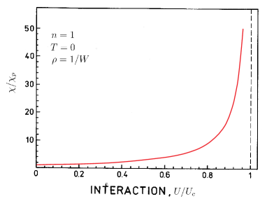
Figure 1: (Color online) Relative static paramagnetic zero-field susceptibility per site ($\chi/\chi_{p}$) as a function of the relative intraatomic interaction strength $U/U_{c}$ for a half-filled narrow band. The divergence marks the Mott-Hubbard localization, called also the Brinkman-Rice instability point.

Apart from the methods used above, we would like to quote the variational method of Gutzwiller wave function (GWF) [48, 49], which represented a contemporary to Hubbard (1963-65) and an independent alternative formulation, also with respect to the Hubbard Hamiltonian introduction. This method has been analyzed extensively starting from the work of Brinkman and Rice in 1970 [50], who showed that a simpler Gutzwiller approximation (GA) produces a divergent static magnetic susceptibility at the metal-insulator transition (MIT). The divergence displayed in Fig. 1 for example of constant density of states, with the critical value for the metal - insulator transition $U_{C}=2W$, what proves that MIT is realized as a continuous quantum phase transformation. Although, the Gutzwiller approximation is exact only for a lattice of infinite dimensions [51, 52], it provides to this day a qualitative border point dividing the narrow-band systems into weakly or moderately correlated systems from one side and those being in the strong correlation regime from the other.

Before considering the strongly correlated systems, we should note one more very important qualitative feature of the Gutzwiller approximation, which survived to these days. Namely, it allowed to introduce a self-consistent procedure of introducing the concept of quasiparticle (the so-called statistical quasiparticle) in the regime $U\gtrsim W$. In this regime, the Landau theory of Fermi liquids in its standard version is inapplicable. In essence, the renormalized quasiparticle energies have the form $E_{\boldsymbol{k}\sigma}=q_{\sigma}\,\epsilon_{\boldsymbol{k}}$, where the band narrowing factor $q_{\sigma}$ is related to the effective mass enhancement, i.e., $m^{*}_{\sigma}/m_{B}=1/q_{\sigma}$, where $m_{B}$ is the bare band mass. Explicitly, we have

$$q_{\sigma}=\frac{\sqrt{n_{\sigma}-d^{2}}\,\sqrt{1-n+d^{2}}+d\sqrt{n_{\bar{\sigma}}-d^{2}}}{n_{\sigma}(1-n_{\sigma})},$$ (5)

where $n_{\sigma}\equiv\langle\hat{n}_{i\sigma}\rangle$ and $d^{2}\equiv\langle\hat{n}_{i\uparrow}\,\hat{n}_{i\downarrow}\rangle$ is the probability of having double occupancy which is determined by minimizing the ground state energy of the system

$$E_{G}/N=\frac{1}{N}\sum_{\boldsymbol{k}\sigma}E_{\boldsymbol{k}}\left\langle\hat{n}_{\boldsymbol{k}\sigma}\right\rangle+Ud^{2},$$ (6)

where at $T=0$ $\langle\hat{n}_{\boldsymbol{k}\sigma}\rangle=\Theta(\mu-E_{\boldsymbol{k}\sigma})$ and $\mu$ is the chemical potential. The parameter $d^{2}$ reaches zero at $U=U_{C}\equiv 8|\bar{\epsilon}|$, where

$$\bar{\epsilon}=\frac{1}{N}\sum_{\boldsymbol{k}\sigma}\epsilon_{\boldsymbol{k}}\left\langle\hat{n}^{0}_{\boldsymbol{k}\sigma}\right\rangle,$$ (7)

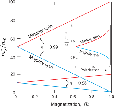
Figure 2: (Color online) The enhancements of spin-split masses $m^{*}_{\sigma}/m_{0}$ for $n<1$ as a function of relative magnetic moment $\bar{m}=m/n$ for the two band fillings specified. The inset shows the corresponding dependence for the electron gas (cf. Spałek and Gopalan, 1990). Note that the majority-spin carriers acquire the bare band mass as the magnetic saturation is reached, whereas those in the spin minority band become extremely heavy and disappear as the state is approached

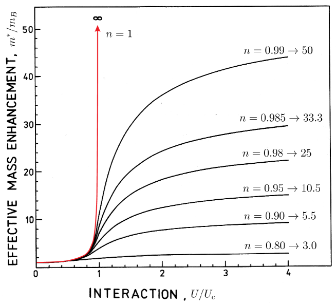
Figure 3: (Color online) Effective mass enhancement versus $U/U_{c}$. On the right: the asymptotic values of $m^{*}/m_{B}$ for $U/U_{c}\rightarrow\infty$ and for selected values of band fillings $n$. All the curves are drawn for a constant form of the density of states ($\rho^{0}(\epsilon)=1/W$, where $W$ is the bare bandwidth.

and $\left\langle\hat{n}^{0}_{\boldsymbol{k}\sigma}\right\rangle\equiv\Theta(\mu^{0}-\epsilon_{\boldsymbol{k}\sigma})$; with $\mu^{0}$ being the chemical potential for bare electrons and $\langle\ldots\rangle$ the statistical distribution and the Fermi energy for bare electrons. In Figs. 2 and 3 we plot the mass enhancement factors for the spin-polarized and paramagnetic states, respectively. Note that the quasiparticle mass is explicitly spin-direction dependent. The quasiparticles in the spin-minority subband become heavier with the increasing polarization, since they scatter on a larger number of (spin-majority) quasiparticles. For the majority-spin carriers the opposite is true.

This picture of self-consistently determined quasiparticle characteristics leads to a number of unique physical properties among them a strong metamagnetism [53] and a nonstandard temperature dependence of the metal-insulator transition [54, 55]. What is more important, with the introduction of the spin-resolved mass differentiation (i.e., the increasing polarization) we reach the limit of distinguishable quasiparticles, for $m^{*}_{\uparrow}\neq m^{*}_{\downarrow}$, out of indistinguishable particles ($m^{*}_{\uparrow}=m^{*}_{\downarrow}=m_{B}$) when the starting state at zero applied magnetic field is paramagnetic [56]. These properties represent a point of departure to the analysis in the strong-correlation limit $U\gg W$. Note that GA in this standard form provides only properties up to maximal value $U=U_{C}\sim W$ (cf. Figs. 1-3). Similar properties can be obtained within the periodic Anderson model in the strong correlation limit  [57]. Analogical conclusions can be obtained also for orbitally degenerate systems [58].

In relation to what has been said above, two methodological remarks are in place. First, the Gutzwiller approximation has been subsequently reformulated in the quantum-field-theoretical languages as the so-called slave boson approach [59, 60, 61]. Within this approach, GA is regarded as a saddle-point approximation. While relying on the GA results in its initial stage, the slave-boson approach removes one of the principal inaccuracies of GA. Namely, within GA the self-consistent procedure of calculating the averages (particularly, in this spin-polarized state) provides results which differ from those obtained from an appropriate variational procedure. This deficiency of the method has been corrected with the introduction of statistically consistent Gutzwiller approximation (SGA), which not only brings into agreement the original results and those of the slave-boson approach in the saddle point approximation, but also avoids introducing the slave (ghost) boson fields which are introduced ad hoc in the latter formulation [62]. In this manner, a consistent mean-field treatment has been formulated, which will be discussed in detail in the context of unconventional superconductivity in the strong-correlation limit which as discussed next.

The reformulation of the Gutzwiller approach in the quasiparticle language [59, 60, 61] has one additional advantage. Namely, it is applicable to the $T>0$ situation.

Second, as the GA approximation has, strictly speaking, precise meaning for high-dimension ($d\rightarrow\infty$) limit, the Brinkman-Rice analysis is often regarded as qualitative at best, i.e., setting the division into regimes of $U<U_{c}$ and $U>U_{c}$ as regimes with qualitatively different physics in each of them. There have been various analytic and numerical trials to allow for an interpolation between those two limits. Apart from extensive an Quantum Monte Carlo analysis, a generalization of the Gutzwiller wave function to include double-holon correlations was proposed [33]. This approach provides better ground state energy and characteristic while preserving the principal physics of GA. However, it leads to the first-order Mott transition, in agreement with our recent SGA analysis [34].

2.4 Strong correlation limit: t-J model

As said above, the starting half-filled-band metal transforms for $U\gtrsim W$ into the Mott (or more precisely, Mott-Hubbard) insulator, which is essentially an antiferromagnet with localized moments. Anderson [63] was the first to point out that the Mott insulating state of e.g., La₂CuO₄ with $3d^{9}$ (spin $S=1/2$) configuration of Cu²⁺ ions can be regarded as the parent material for the high temperature superconductor La_2-xSr_xCuO₄ (LSCO) which appears for the doping $x\gtrsim 0.05$, with the deficient electrons effectively producing Cu^2+x configurations of itinerant holes in this doped Mott insulator. The effective Hamiltonian known nowadays under the acronym of "t-J model" was derived originally by us [36, 37, 38] for an arbitrary band filing $n$ (hole doping $x\equiv 1-n$) and has the form

$$\widetilde{\mathcal{H}}=\sum_{ij\sigma}\!^{{}^{\prime}}t_{ij}\,\hat{b}_{i\sigma}^{\dagger}\,\hat{b}_{j\sigma}+\sum_{ij}\!^{{}^{\prime}}\frac{2t_{ij}^{2}}{U}\left(\widehat{\boldsymbol{S}}_{i}\cdot\widehat{\boldsymbol{S}}_{j}-\frac{c_{1}}{4}\,\widehat{\nu}_{i}\,\widehat{\nu}_{i}\right)$$

$$+\sum_{ijk\sigma}\!^{{}^{\prime\prime}}\,\frac{t_{ij}\,t_{jk}}{U}\,c_{2}\left(\hat{b}_{i\sigma}^{\dagger}\,\widehat{\nu}_{j\bar{\sigma}}\,\hat{b}_{k\sigma}-\hat{b}_{i\sigma}^{\dagger}\,\widehat{S}_{j}^{\bar{\sigma}}\,\hat{b}_{k\bar{\sigma}}\right),$$ (8)

where the single-primed summation means that $i\neq j$, the double-primed means that $i\neq j\neq k\neq i$. Also, $\hat{b}_{i\sigma}^{\dagger}\equiv\hat{a}_{i\sigma}^{\dagger}(1-\widehat{n}_{i\bar{\sigma}})$, $\hat{\nu}_{i\sigma}\equiv\hat{b}^{\dagger}_{i\sigma}\,\hat{b}_{i\sigma}=\hat{n}_{i\sigma}(1-\widehat{n}_{i\bar{\sigma}})$ are the projected fermionic operators, $\widehat{\boldsymbol{S}}_{i}\equiv(\widehat{S}_{i}^{z},\widehat{S}_{i}^{\sigma})$ is the spin operator in the fermion representation. The first term represents a restricted hopping, with the double occupancies projected out, the remaining two terms represent respectively the second-order processes and contain virtual-hopping processes to the double occupancies configuration (for the didactical exposition see e.g., [64, 65]). The extra parameters $c_{1},c_{2}=0,1$ are introduced to model the system with and without of the corresponding terms respectively [66].

At the times, this Hamiltonian was used to describe mainly magnetic properties (mainly ferromagnetism) at or near the Mott insulating limit [67, 68, 69]. In other words, only the moving correlated spins have been seen in this unusual situation with the double-site occupancies being ruled out . As those moving spins avoid each other ($\langle\widehat{n}_{i\uparrow}\,\widehat{n}_{i\downarrow}\rangle\equiv 0$), the intersite antiferromagnetic interaction (the second term) produces strong pair spin-singlet correlations, that can produce either a long-range antiferromagnetism, or a liquid of pair spin singlets entangled with the hole hopping. This last state is sometimes termed a resonating-valence-bond (RVB) state [70, 71]. However, since in the correlated state the renormalized hoping magnitude is $t_{ij}\rightarrow t_{ij}x$ and the corresponding kinetic-exchange integral is $J_{ij}\equiv 2t_{ij}^{2}/U\rightarrow J_{ij}(1-x)^{2}$, for $x\lesssim~{}0.1$ the exchange term becomes predominant and the hopping strongly suppressed, what produces an insulating antiferromagnetic state as $x\rightarrow 0$. Such was the state of affairs until 1986.

The invention of real space pairing [63, 39, 40] has introduced the completely new aspects to the problem. First, one can introduce explicit the real-space spin-singlet pairing operators in a rigorous manner in the form [40]

$$\left\{\begin{array}[]{l}B_{ij}^{\dagger}\equiv\frac{1}{2}\left(\hat{b}_{i\uparrow}^{\dagger}\>\hat{b}_{j\downarrow}^{\dagger}-\hat{b}_{i\downarrow}^{\dagger}\>\hat{b}_{j\uparrow}^{\dagger}\right),\\ B_{ij}\equiv\frac{1}{2}\left(\hat{b}_{i\uparrow}\>\hat{b}_{j\downarrow}-\hat{b}_{i\downarrow}\>\hat{b}_{j\uparrow}\right)\end{array}\right.$$ (11)

and cast the effective Hamiltonian (8) in the following closed form [40]

$$\widetilde{\mathcal{H}}=\sum_{ij\sigma}\!^{{}^{\prime}}t_{ij}\>\hat{b}_{i\sigma}^{\dagger}\>\hat{b}_{j\sigma}-\sum_{ijk}\!^{{}^{\prime}}\,\frac{4t_{ij}\>t_{jk}}{U}B_{ij}^{\dagger}\>B_{kj}.$$ (12)

From this expression one can see explicitly that a nonzero number of local singlet pairs $\langle B_{ij}^{\dagger}\,B_{ij}\rangle$ diminishes the system energy and additionally, in the Hartree-Fock-like factorization of the Bogoliubov type: $\langle B_{ij}^{\dagger}\rangle\,\langle B_{ij}\rangle$, the quantity $\langle B_{ij}^{\dagger}\rangle$ is the real-space correspondant of the order parameter in the Barden-Cooper-Schrieffer (BCS) theory, $\Delta_{\boldsymbol{k}}\equiv\langle\hat{a}_{\boldsymbol{k}\uparrow}^{\dagger}\,\hat{a}_{-\boldsymbol{k}\downarrow}^{\dagger}\rangle$. However, there is one principal difference: in the present situation we have $\langle B_{ii}^{\dagger}\rangle\equiv 0$ rigorously due to the Gutzwiller projection and therefore, the gap parameter cannot have a scalar ($\boldsymbol{k}$-independent) $s$-wave form. Instead, in the simplest situation it must have either the extended $s$-wave or the $d$-wave form [72]. These forms are the simplest representations of the intersite character of the pairing amplitude $\langle B_{ij}^{\dagger}\rangle$.

The second factor was the discussion of electronic states for CuO₂ plane in LSCO a subsequent reintroduction [63, 41] of the t-J model with $J_{ij}$ not limited to the asymptotic expression for $|t_{ij}|\ll U$ appearing as (8). In effect, that value of the ratio $J/|t|$ within such redefined effective t-J model is usually taken for the nearest neighbors as $J/|t|=0.3$. This ratio value is assumed in the following, when illustrating the theoretical results with a detailed numerical analysis.

A methodological note is in place here. The representations (8) and (12) are simply equivalent. Hence the motion of the local singlets in the paired state, as provided by the second term in (12) and the correlated hoping of holes must cooperate with each other in forming such a condensed state of moving pairs. Such cooperation of the two factors has been proposed recently [74].

3 Description of the high-$T_{C}$ superconducting state

3.1 Statistically consistent mean-field approach (SGA)

The standard approach to the description of superconducting state starting from (12) is the so-called renormalized mean field theory (RMFT) [73, 74, 75]. However, as we have noticed [62, 66, 77, 78] the additional constraints must be reintroduced so that the averages appearing in the effective single-particle Hamiltonian and calculated self-consistently coincide with those determined by an alternative variational approach. This is the basic principle which must be obeyed by any consistent approach from the statistical physics point of view. In result, the effective single-particle Hamiltonian for $c_{1}$ and $c_{2}=0$ reads:

$$\mathcal{H}= \sum_{ij\sigma}\left(t_{ij}\,g_{ij}^{t}\,\hat{a}_{i\sigma}^{\dagger}\,\hat{a}_{j\sigma}+\text{H.c.}\right)-\mu\sum_{i\sigma}\hat{a}_{i\sigma}^{\dagger}\,\hat{a}_{i\sigma}$$

$$- \frac{3}{4}\sum_{ij\sigma}J_{ij}\,g_{ij}^{J}\left(\chi_{ij}\,\hat{a}_{i\sigma}^{\dagger}\,\hat{a}_{j\sigma}+\text{H.c.}-|\chi_{ij}|^{2}\right)$$

$$- \frac{3}{4}\sum_{ij\sigma}J_{ij}\,g_{ij}^{J}\left(\Delta_{ij}\,\hat{a}_{i\sigma}^{\dagger}\,\hat{a}_{j\bar{\sigma}}^{\dagger}+H.c.-|\Delta_{ij}|^{2}\right),$$ (13)

where $\chi_{ij}\equiv\langle\hat{a}_{i\sigma}^{\dagger}\,\hat{a}_{j\sigma}\rangle$ and $\Delta_{ij}\equiv\langle\hat{a}_{i\bar{\sigma}}\,\hat{a}_{i\sigma}\rangle$ are respectively the hopping amplitude and the pairing other parameter. The renormalization factors $g_{ij}^{t}$ and $g_{ij}^{J}$ result from the Gutzwiller approximation. Additionally, when the statistical-consistency conditions [77, 78] are included, the Hamiltonian can be written in the form

$$\mathcal{H}_{\lambda} =W-\sum_{\langle ij\rangle\sigma}\widetilde{\eta}_{ij\sigma}\left[\left(\hat{a}_{i\sigma}^{\dagger}\,\hat{a}_{j\sigma}-\chi_{ij\sigma}\right)+\text{H.c.}\right]$$

$$-\sum_{\langle ij\rangle}\widetilde{\gamma}_{ij}\left[\left(B_{ij}-\Delta_{ij}\right)+\text{H.c.}\right]-\sum_{i\sigma}\widetilde{\lambda}_{ni}\left(\widehat{n}_{i\sigma}-n_{i\sigma}\right),$$ (14)

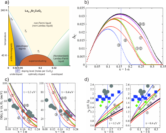
Figure 4: (Color online) a) representative phase diagram for cuprate high $T_{C}$ superconductors: $T_{p}$ means pseudogap characteristic temperature and $T_{C}$ is the critical temperature for superconducting phase transition; b) theoretical phase diagram specifying only the superconductivity to normal metal transition; c) the gap amplitude versus doping $x$ in the antinodal ($k_{x},0$) direction for the two values of the nearest neighbor parameter $t\equiv|t|$ specified; d) Fermi velocity versus $x$ in the nodal direction $k_{x}=k_{y}$; note the systematic derivation in the underdoped regime (the optimal doping is marked on Figs. b-d as a vertical line).

where $W\equiv\langle\mathcal{H}\rangle$ means the mean-field expectation value of (13) and the last three terms represent the Lagrange constraints with the corresponding multipliers $\widetilde{\eta},\widetilde{\gamma}$, and $\widetilde{\lambda}$. In the case of spatially homogeneous state the solution reduces to solving a system of 6 algebraic (integral) equations. The results obtained in this manner have been displayed in the panel composing Figs. 4b-d [66, 78]. For the sake of completeness, in Fig. 4a we present a schematic phase diagram obtained experimentally and encompassing the doping regime $0.055\lesssim x\lesssim 0.35$, where the superconducting state is stable.

Few features of the whole approach should be noted. First, the approach contains the correlated gap parameter $\Delta_{c}\equiv\langle B_{ij}\rangle\equiv g_{t}\,\Delta_{ij}$, the correlated hopping amplitude $\langle(g^{t}\,\chi_{ij})\rangle$, and the renormalized exchange integral ($g^{s}J_{ij}$), where $g^{t}$ and $g^{J}$ are the renormalization factors due to correlations:

$$g_{ij}^{t}=\sqrt{\frac{4x_{i}\,x_{j}(1-x_{i})(1-x_{j})}{\left(1-x_{i}^{2}\right)\left(1-x_{j}^{2}\right)+8(1-x_{i}\,x_{j})|\chi_{ij}|^{2}+16|\chi_{ij}|^{4}}},$$ (15)

$$g_{ij}^{J}=\frac{4(1-x_{i})(1-x_{j})}{\left(1-x_{i}^{2}\right)\left(1-x_{j}^{2}\right)+8x_{i}\,x_{j}\,\beta_{ij}^{-}(2)+16\beta_{ij}^{\dagger}(4)},$$ (16)

with $x_{i}\equiv 1-n_{i}$ and $\beta_{ij}^{\pm}(n)\equiv|\Delta_{ij}|^{n}\pm|\chi_{ij}|^{n}$.

Second, as noted earlier, Eq. (14) defines the correct renormalized mean-field approach in the sense that the average fields $\Delta$ and $\chi$, derived from self-consistent equations coincide with those obtained variationally from the appropriate Landau functional obtained from (14) [66] . In this manner, the Bogoliubov-Feynman variational principle is obeyed.

The results displayed in Figs. 4b-d are drawn for different sets of model parameters (for details see [78]). Irrespectively of the quantitative differences, few universal trends should be noted. First, there is a well defined upper critical concentration contained in the regime of $x=1/4\div 1/3$, in agreement with experimental results shows in Fig. 4a. The presence of the upper critical concentration for disappearance of superconductivity has been interpreted by us a signature of real space pairing [74]. Simply put, with the increasing hole doping the pairs get diluted to the extent of destroying the condensed state. Second, the trend of the data concerning the evolution with $x$ of the gap parameter $\Delta_{\langle ij\rangle}$ in the antinodal ($k_{x},0$) direction is also reflected in trend of the theoretical results. However, there is a problem with the $x$-dependence of the Fermi velocity in the nodal direction ($k_{x}=k_{y}$), as the experimental values are only weakly dependent on $x$. On the other hand, the theoretical data reflected the trend characteristic of a Fermi liquid, for which the diminishing Fermi velocity with the decreasing $x$ is easy to understand. Therefore, the feature of the data collected in Fig. 4d speaks in favor of a non-Fermi liquid and/or higher-order effects becoming eminent in the underdoped regime. We address this discrepancy by discussing next the Gutzwiller-wave-function diagrammatic expansion (DE-GWF) in the next Section.

3.2 Beyond the renormalized mean-field approach: systematic diagrammatic expansion for the Gutzwiller-wave-function approach

As said above, the Gutzwiller variational-method origin can be traced to the independent Hubbard-model inception [48, 49]. During the first 10 years (1965-1975), the Gutzwiller approximation (ansatz) was used frequently. After that period, a systematic (iterative) solution for the full Gutzwiller wave-function has been achieved, first for a one dimensional case [79, 80]. A generalization of this solution to the case of two spatial dimensions via systematic diagrammatic expansion has been undertaken recently for both normal [81] and superconducting [82, 83] states. In this brief overview we turn our attention to the most general features of the approach (for details see [83]) and then concentrate on comparison with experiment.

The essence of developing a systematic expansion beyond any mean-field approximation is as follows. In any variational procedure we would like to calculate the optimal grand-state energy $\langle\Psi|H|\Psi\rangle$. In the presence approach

$$|\Psi\rangle\equiv|\Psi_{G}\rangle=\widehat{P}\,|\Psi_{0}\rangle=\prod_{i}\widehat{P}_{i}\,|\Psi_{0}\rangle$$ (17)

where $\widehat{P}_{G}$ is the Gutzwiller projection operator, here taken in the form [84]

$$\widehat{P}_{i}=\sum_{\Gamma}\lambda_{i,\Gamma}\,|\Gamma\rangle_{i}\,{}_{i}\langle\Gamma|,$$ (18)

with variational parameters $\lambda_{i,\Gamma}$ describing the occupation probabilities of four possible local (site) configurations represented by the corresponding states, $\{|\Gamma\rangle_{i}\}\equiv\{|\emptyset\rangle_{i},|\!\uparrow\rangle_{i},|\!\downarrow\rangle_{i},|\!\uparrow\downarrow\rangle_{i}\}$. A choice of $\{\lambda_{i\Gamma}\}$ selected here provides the following form of the local projection operator

$$\widehat{P}_{i}^{2}\equiv 1+\tilde{x}\,\widehat{d}_{i}^{HF},$$ (19)

where $\tilde{x}$ is a variational parameter and $\widehat{d}_{i}^{HF}=(\widehat{n}_{i\uparrow}-\widehat{n}_{i\uparrow}^{0})(\widehat{n}_{i\downarrow}-\widehat{n}_{i\downarrow}^{0})$, with $\langle n_{i\sigma}^{0}\rangle=\langle\Psi_{0}|\widehat{n}_{i\sigma}|\Psi_{0}\rangle$. With this form of the projection operator one sees that the ground states energy can be expressed as

$$\langle\mathcal{H}\rangle=\frac{\left\langle\Psi_{0}\left|\widehat{P}\,\mathcal{H}\,\widehat{P}\right|\Psi_{0}\right\rangle}{\left\langle\Psi_{0}\left|\,\widehat{P}^{2}\,\right|\Psi_{0}\right\rangle}.$$ (20)

So the evolution of the expectation value of $\mathcal{H}$ reduces to calculation of those for $\widehat{P}\,\mathcal{H}\,\widehat{P}$ and $\widehat{P}^{2}$ in the $|\Psi_{0}\rangle$ which represents (and is dependent on the problem and hand) single-particle wave function $|\Psi_{0}\rangle$. This simplifies remarkably the calculations, as the averages can be factorized into products of simpler pair correlation functions using the Wick theorem in real space. An efficient method of evaluating systematically the averages, including the pairing correlations, has been overviewed in detail elsewhere in this issue [85]. Here we summarize only the main results.

The averages in (20) involve only the wave function $|\Psi_{0}\rangle$ representing an uncorrelated state. Therefore, one can define an effective Hamiltonian $\widehat{\mathcal{H}}_{0}^{\rm eff}$ for which this state is an eigenstate. A detailed analysis shows that both in the case of Hubbard [82] and t-J [83] model cases one can define the effective single-particle Hamiltonian of the form:

$$\widehat{\mathcal{H}}_{0}^{\rm eff} = \sum_{\boldsymbol{i},\boldsymbol{j},\sigma}t^{\rm eff}_{\boldsymbol{i},\boldsymbol{j}}\,\hat{c}_{\boldsymbol{i},\sigma}^{\dagger}\,\hat{c}_{\boldsymbol{j},\sigma}^{\phantom{\dagger}}+\sum_{\boldsymbol{i},\boldsymbol{j}}\left(\Delta^{\rm eff}_{\boldsymbol{i},\boldsymbol{j}}\,\hat{c}_{\boldsymbol{i},\uparrow}^{\dagger}\,\hat{c}_{\boldsymbol{j},\downarrow}^{\dagger}+\text{H.c.}\right),$$ (21)

$$t^{\rm eff}_{\boldsymbol{i},\boldsymbol{j}} = \frac{\partial\mathcal{F}\!\left(|\Psi_{0}\rangle,x\right)}{\partial P_{\boldsymbol{i},\boldsymbol{j}}}\;,\qquad\Delta^{\rm eff}_{\boldsymbol{i},\boldsymbol{j}}=\frac{\partial\mathcal{F}\!\left(|\Psi_{0}\rangle,x\right)}{\partial S_{\boldsymbol{i},\boldsymbol{j}}}\;.$$ (22)

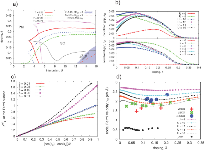
Figure 5: (Color online) a) Stability regime on plane interaction $U-$ doping$\delta$ for specified values of the parameters (in the lower right corner the BCS vs. non-BCS regimes, see main text); b) superconducting gap magnitude vs. $\delta$ for different $U$ (the lower panel: the convergence with the order $k$ of thr DE-GWF expansion) c) correction to the poor d-wave gap due to longer-range pairing components (the black solid line marks a purse d-wave character); d) Fermi velocity vs. $\delta$: the upper set of points are the are the some experimental data as in Fig. 4d, whereas the lower solid points represent DMFT results. For details see Ref. [82]

where $P_{\boldsymbol{i},\boldsymbol{j}}\equiv\langle\psi_{0}|\hat{c}_{i\sigma}^{\dagger}\,\hat{c}_{j\sigma}|\psi_{0}\rangle-\delta_{ij}\langle\Psi_{0}|\hat{n}_{i\sigma}|\Psi_{0}\rangle$, $S_{ij}\equiv\langle\psi_{0}|\hat{c}_{i,\uparrow}^{\dagger}\,\hat{c}_{j,\downarrow}^{\dagger}|\psi_{0}\rangle$ and $\mathcal{F}\equiv\langle\psi|\mathcal{H}|\psi\rangle_{G}-2\mu_{G}\,n_{G}$ with $n_{\sigma}\equiv\langle\Psi_{G}|\hat{n}_{i\sigma}|\Psi_{G}\rangle$ is the generalized grand-canonical potential in the GWE state. One see that (21) is the effective single-particle Hamiltonian with BCS-type pairing in the real space-language. This equation contains a number of parameters to be determined self-consistently: $P_{i,j},\Delta_{i,j},\mu$, and $n_{G}$ (for a detailed discussion see Refs. [82, 83]). In Fig. 5a-d we have assembled the principal results of the approach.

Explicitly, Fig 5a illustrates the two features of the solution. First, superconducting state appears only at sufficiently high $U$ ($U\equiv U/|t|\gtrsim 3$). This shows explicitly that in obtaining a stable superconducting solution the electron correlations must be taken into account, as there is no such solution in the Hartree-Fock approximation. Also, the BCS/non-BCS boundary specifies the shaded regime in the lower right-hand corner, where the kinetic energy ($\Delta E_{kin}$) is lowered in the superconducting phase. The line within the shaded regime marks the situation in which the potential energy gain forming SC phase is zero, a clearly non-BCS feature. In Fig. 5b we displayed evolution of the doping dependence of the correlated gap with the increasing $U$. We see that for sufficient high $U$-value, the system transforms into the Mott insulator at $\delta=0$, as it should be. The lower panel on that figure demonstrates the convergence of the results for $\Delta_{G}$ with the ascending order of the DE- GWF expansion. The results for $k=4$ and $k=5$ practically coincide, a rewarding feature in view of the intricacy of the expansion [85]. In Fig. 5c we draw the $\boldsymbol{k}$-dependence of the gap and, in particular, demonstrate the deviation from a pure $d$-wave solution for $\Delta_{\boldsymbol{k}}$ away from the optimal doping. This type of behavior is observed experimentally [86], though a quantitative comparison with experiment would involve also determination of the doping dependence of the pseudogap. Finally, in Fig. 5d the Fermi velocity is plotted against $\delta$, with the same experimental points, as in Fig. 4d. We see that the theory reflects now to much better extent the trend of the experimental data in the last Figure. Indeed, DE-GWE approach represents more advanced approach than SGA. It should be underlined though that while the plots Fig. 4 illustrate the SGA results for t-J model, those in Fig. 5 are obtained for the Hubbard model. What is important, SGA does not produce a stable superconducting state within the Hubbard model.

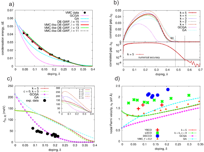
Figure 6: (Color online) Characteristics of the paired superconducting state coming from the t-J model and obtained in DE-GWF method [83] as a function of hole doping $x=\delta$: a) condensation energy compared with variational Monte-Carlo (VMC) and VMC-like results, the latter contain the diagrams with a $l=15,13$, and 11 lines; the lowest curve represents SGA results, whereas the black points those from VMC; b) the correlated gap in the different order of the DE-GWF expansion (the lowest one represents SGA results); the lower part shows the numerical accuracy of $\Delta_{G}$ evaluation in both $\delta\rightarrow 0$ and $\delta>0.4$; c) the gap amplitude in the antinodal direction in different orders (the lowest curve represents SGA results and is close to the experimental results; d) universal Fermi velocity in the nodal direction and its comparison to experiment.

Recently, we have also reanalyzed the t-J model within the DE-GWF approach (for details see [83]) and the results are of similar character as those for the Hubbard model. Explicitly, in Figs. 6a-d we summarize those results and compare them to those obtained in Variational Monte-Carlo (VMC) method (cf. Fig. 6a). Figs. 6b-d can be directly compared to those of Figs. 4b-d. Here SGA $\equiv$ GCGA (grand canonical Gutzwiller approximation). One can see that the $v_{F}(\delta)$ dependence is best reproduced within the Hubbard model (cf. Fig. 5d).

On the basis of the results depicted in Figs. 3-5 we see that the strong correlations are necessary to reproduce an overall behavior. Note that the lowest points in Fig. 4d are those obtained from DMFT approach [87] for the same values of the parameters. Additionally, the results presented here are of the same quality as those obtained from Variational Monte Carlo method [83]. All these features prove that the DE-GWF (starting from SGA as the lowest order) is a reliable method for treating the high-temperature superconductivity, at least its overall features.

4 From Anderson to Anderson-Kondo lattice

4.1 Anderson-Kondo lattice

At the end we overview briefly the evolution of the Anderson-lattice model from description of quasiparticle states in heavy-fermion systems and their magnetism to the discussion of paired superconducting states. To model the heavy fermion systems, such as the compounds with cerium (with approximate $4f^{1}$ configuration of Ce^3+δ ions), we start from the two-orbital Anderson lattice model, which is the real-space representation has the following form:

$$\mathcal{H}= \sum_{mn\sigma}\,t_{mn}\,\hat{c}^{\dagger}_{m\sigma}\,\hat{c}_{n\sigma}+\epsilon_{f}\sum_{i\sigma}\hat{N}_{i\sigma}+U\sum_{i\sigma}\hat{N}_{i\uparrow}\,\hat{N}_{i\downarrow}$$ (23)

$$+\sum_{im\sigma}\left(V_{im}\,\hat{f}^{\dagger}_{i\sigma}\,\hat{c}_{m\sigma}+\text{H.c.}\right)-\mu\left(\sum_{i\sigma}\hat{N}_{i\sigma}+\sum_{m\sigma}\hat{n}_{m\sigma}\right),$$

where $\hat{N}_{i\sigma}\equiv\hat{f}^{\dagger}_{i\sigma}\,\hat{f}_{i\sigma}$ is the number of $f$ electrons on site $i$ with spin $\sigma$, and $\hat{n}_{m\sigma}\equiv\hat{c}^{\dagger}_{m\sigma}\,\hat{c}_{m\sigma}$ is the corresponding number of the conduction ($c$) electrons. The meaning of the consecutive terms is as follows: the first term expresses band (hoping) energy of $c$-electrons; the second, the starting atomic energy of $f$ electrons (with their level position $\epsilon_{f}$); the third the $f$-$f$ intraatomic (Hubbard) interaction; the fourth the $f$-$c$ hybridization (with amplitude $V_{im}$); and the last, the corresponding chemical potential part, as we work in the grand-canonical formalism.

In the interesting us regime of strong correlations the parameter $U$ represents the highest energy scale in the system. In the regime, when the emerging quasi-particle states involve itineracy of $f$ electrons, neither the RKKY $f$-$f$ interaction [2] nor the Schrieffer-Wolff transformation [19] of the Anderson-lattice model to the effective Kondo-lattice model, are applicable. Instead, at best one can invoke the concept of the Anderson-Kondo lattice, which we explain in detail and apply subsequently to the description of paired states.

It is important to note that while the ratio $|V|/(U+\epsilon_{f})\ll 1$, the relative hybridization strength $V/\epsilon_{f}$ cannot be regarded as small and therefore transformed out, as would be the case in the situation with the Schrieffer-Wolff transformation. This circumstance leaves us always with a residual hybridization even when we transform canonically the starting Hamiltonian (23) into that containing the Kondo-type interaction in an explicit form. Leaving the details of such transformation aside [88, 23, 22], the effective Hamiltonian under these assumptions has the form

$$\mathcal{H}= \mathcal{\hat{P}}\left\{\sum_{mn\sigma}\left(t_{mn}\,\hat{c}^{\dagger}_{m\sigma}\,\hat{c}_{n\sigma}-\sum_{i}\frac{V_{im}^{*}\,V_{in}}{U+\epsilon_{f}}\,\hat{\nu}_{i\bar{\sigma}}\,\hat{c}^{\dagger}_{m\sigma}\,\hat{c}_{n\sigma}\right)\right\}\mathcal{\hat{P}}$$

$$+ \mathcal{\hat{P}}\left\{\sum_{imn\sigma}\frac{V_{im}^{*}\,V_{in}}{U+\epsilon_{f}}\,\hat{S}_{i}^{\sigma}\hat{c}^{\dagger}_{m\bar{\sigma}}\,\hat{c}_{n\sigma}+\sum_{i\sigma}{\epsilon_{f}}\,\hat{\nu}_{i\sigma}\right\}\mathcal{\hat{P}}$$

$$+ \mathcal{\hat{P}}\left\{\sum_{im\sigma}\left(1-\hat{N}_{i\bar{\sigma}}\right)\left(V_{im}\,\hat{f}^{\dagger}_{i\sigma}\,\hat{c}_{m\sigma}+\text{H.c.}\right)\right\}\mathcal{\hat{P}}$$

$$+ \mathcal{\hat{P}}\left\{\sum_{im\sigma}\frac{2|V_{im}|^{2}}{U+\epsilon_{f}}\left(\boldsymbol{\hat{S}}_{i}\cdot\boldsymbol{\hat{s}}_{m}-\frac{\hat{\nu}_{i}\,\hat{n}^{c}_{m}}{4}\right)\right\}\mathcal{\hat{P}}$$

$$+ \mathcal{\hat{P}}\left\{\sum_{ij}J_{ij}\left(\boldsymbol{\hat{S}}_{i}\cdot\boldsymbol{\hat{S}}_{j}-\frac{\hat{\nu}_{i}\,\hat{\nu}_{j}}{4}\right)\right\}\mathcal{\hat{P}}.$$ (24)

Note that in the hybridization term we have projected out only the processes with the double $f$-level occupancies (cf. third line), whereas both the effective Kondo ($f$-$c$) (the fourth line) and $f$-$f$ exchange (superexchange) interaction (the last line) appear in an explicit form as higher-order processes. One should underline that the form (24) should contain the same physics as (23) in the limit we call the Anderson-Kondo limit. However, as we see shortly, it provides physically appealing solutions already within a relatively simply approximation scheme.

Before discussing the results, we introduce explicitly the real-space pairing operators in the following manner

$$\left\{\begin{aligned} \hat{b}^{\dagger}_{im}&\equiv\frac{1}{\sqrt{2}}\left(\tilde{f}^{\dagger}_{i\uparrow}\,\hat{c}^{\dagger}_{m\downarrow}-\tilde{f}^{\dagger}_{i\downarrow}\,\hat{c}^{\dagger}_{m\uparrow}\right)\equiv(\hat{b}_{im})^{\dagger},\\ \hat{B}_{ij}^{\dagger}&\equiv\frac{1}{\sqrt{2}}\left(\tilde{f}_{i\uparrow}^{\dagger}\,\tilde{f}_{j\downarrow}^{\dagger}-\tilde{f}_{i\downarrow}^{\dagger}\,\tilde{f}_{j\uparrow}^{\dagger}\right)=\left(\hat{B}_{ij}^{\dagger}\right)^{\dagger},\end{aligned}\right.$$ (25)

where $\tilde{f}_{j\sigma}\equiv\hat{f}_{i\sigma}(1-\hat{N}_{i\bar{\sigma}})$ and $\hat{\nu}_{j\sigma}\equiv\hat{N}_{i\sigma}(1-\hat{N}_{i\bar{\sigma}})$. In effect, the Hamiltonian (24) can be rewritten in a closed form

$$\mathcal{H}= \sum_{mn\sigma}t_{mn}\,\hat{c}^{\dagger}_{m\sigma}\,\hat{c}_{n\sigma}+\epsilon_{f}\sum_{i\sigma}\hat{\nu}_{i\sigma}+\sum_{im\sigma}\left(V_{im}\,\tilde{f}^{\dagger}_{i\sigma}\,\hat{c}_{m\sigma}+\text{H.c.}\right)$$ (26)

$$-\sum_{imn}\frac{2V^{*}_{im}\,V_{in}}{U+\epsilon_{f}}\,\hat{b}^{\dagger}_{im}\,\hat{b}_{in}-\sum_{ij}J_{ij}\,\hat{B}^{\dagger}_{ij}\,\hat{B}_{ij}.$$

The first term in the second line represents the so-called hybrid real-space pairing and express the Kondo-type spin-singlet correlations, whereas the second the corresponding $f$-$f$ pairing of the type considered already in the context of t-J model. The real-space pairing parts diminishe the system energy in the spin-singlet paired state. The pairing $\hat{b}^{\dagger}\hat{b}$ introduces the hybrid ($f$-$c$) local-pair contribution and $\hat{B}^{\dagger}\hat{B}$ expresses the corresponding local $f$-$f$ binding. Those two types can compete and lead to a frustration effects in the paired state.

4.2 Magnetic and paired states: phase diagram

The Hamiltonian has been solved within the SGA scheme [22, 23] and some of the results (and the whole method) are over-viewed briefly in Fig. 7a-d. Namely, in Fig 7a we visualize the basis on which the transformation from (23) to (24) has been carried out. The high-energy processes lead to the $f$-$c$ and $f$-$f$ exchange interactions; the low-energy correspondants represent the residual hybridization. Fig. 7b illustrates that, strictly speaking, three physically distinct regimes in large-$U$ limit should be singled out, as specified, with the increasing ratio $V/\epsilon_{f}$. In Fig. 7c we show exemplary result in the Kondo-insulator regime (for $n_{e}=2$), where the quantum critical point (QCP) appears between the antiferromagnetic Kondo insulator (AKI) and the nonmagnetic Kondo insulator (PKI), the latter with totally compensated magnetic moments of $f$ ($m_{f}$) and $c$ ($m_{c}$) electrons. One should emphasize that such a completely compensated state is due to the two factors: the antiferromagnetic Kondo interaction from one side and the autocompensation of itinerant character of $f$ electrons combined with the antiferromagnetic kinetic exchange between them from the other. The inset shows the diminishing $f$-level occupancy $n_{f}\equiv\sum_{\sigma}\langle\hat{\nu}_{i\sigma}\rangle$ with the increasing strength of the (intraatomic in this case) hybridization.

Finally, in Fig. 7d we provide the overall phase diagram, this time for the case with hybridization between the nearest-neighboring pairs $\langle i,m\rangle$. The superconducting solution is of the $d$-wave type, both for the hybrid and $f$-$f$ Cooper pairs. The sequence of the phases with the increasing nearest-neighbor hybridization amplitude $|V|=|V_{\langle i,m\rangle}|$ is as follows. For small hybridization the strong (SFM) and the weak (WFM) ferromagnetic phases appear in this regime of practically localized $f$ electrons ($n_{f}>0.9$). A purely antiferromagnetic (AF) phase is sandwiched in between the mixed antiferromagnetic-superconducting (AF+SC) phases. For large enough $|V|$, a pure superconducting phase emerges in the fluctuating-valence regime, $n_{f}\simeq 0.8$. The sequence of the phases near QCP (the black solid dots in Figs. 7c and d) reflects (inverted $"V"$) quantum-critical behavior appearing in the quasi-two-dimensional heavy-fermion system [89] (the results are calculated for the case of square lattice), dividing the AF and SC phases, and with AF+SC phase inside.

Concluding this Section, the Anderson-Kondo lattice model leads to a number of magnetic and superconducting phases, both induced by the magnetic interactions and the interelectronic correlations combined. A separate question concerns the DE-GWF generalization for the Anderson-Kondo lattice [90], but this topic will not be touched upon here.

5 Outlook

In this brief overview we have put an emphasis on the connection between magnetic and superconducting states, both treated on the same footing and within a single model of correlated fermions. In other words, no extra fermion-boson interaction is necessary to introduce both magnetism and/or unconventional superconductivity. The question is to what extent the above models conceived more than 50 years ago convey still novel and relevant physics of many-particle systems. One may say that what wee still need is their systematic analysis for the case of periodic lattices, particularly for orbitally degenerate cases of $d$ and $f$ states. This goal should lead to a formulation of universality classes for continuous quantum phase transitions, definition of the upper and the lower critical dimensions for them, as well as a unified view of the spin correlations in strongly correlated fermionic systems and their relation to the pairing in high-temperature and heavy-fermion superconductors. The quantum Monte-Carlo methods in this respect provide a crucial testing ground for various approximate analytical/numerical solutions in the situation of small systems, but the final goal is to have the solution for extended (infinite) systems. Whether in achieving this goal we should have first a renormalized single-particle approach along the lines discussed here, remains still to be seen. For example, apart from a single result shown in Fig. 7c, no quantum criticality in the low-$U$ limit has has been touched upon here [91, 92, 93]. The consideration of quantum criticality leads to new physics (non-Fermi liquid behavior), for both models. Also, the particular questions of the pseudogap appearance [94] in high-$T_{c}$ systems and, e.g., the hidden-order existence in URu₂Si₂ [95], are not tackled here. Nonetheless, I firmly believe that the considerations touched upon here provide a first if not substantial step in understanding theoretically the superconductivity in the strong-correlation limit for the narrow-band fermions.

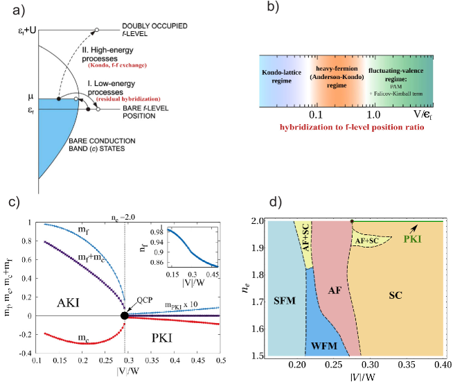
Figure 7: (Color online) a) Schematic representation of hybridization $c$-$f$ process division into the low- and high-energy processes; b) Various physical regimes for Anderson-lattice model with the increasing $V/\epsilon_{f}$ ratio; c) The compensation of the magnetic moment ($m_{f}$) by that of conduction electrons ($m_{c}$) in the state with itinerant $f$-quasiparticles; d) overall phase diagram on the plane number of electrons per pair of orbits ($n_{e}$) -hybridization strength ($|V|$). For details see main text and Ref. [23]

References

- [1] T. Holstein and H. Primakoff, Phys. Rev. 58 1098 (1940)
- [2] K. Yosida, Theory of Magnetism (Springer Verlag, Berlin, 1998) chapter 9
- [3] J. Schwinger, Quantum Theory of Angular Momentum, ed. by L. Biedenharn, (Academic, Press, New York, 1965) pp. 229-279
- [4] N. N. Bogoliubov. Lectures on Quantum Statistics (Gordon and Breach Sci. Publ., New York, 1967) vol. 1
- [5] J. Bardeen, L. N. Cooper, and J. R. Schrieffer, Phys. Rev. 108 (5), 1175 (1957)
- [6] BCS: 50 years, edited by L. N. Cooper, and D. Feldman (World Scientific, New Jersy, 2011)
- [7] H. Fröhlich, Proc. Phys. Soc. A 63, 778 (1950).
- [8] Bardeen and D. Pines Phys. Rev. 99, 1104 (1955)
- [9] S. Pekar, J. Phys. (U.S.S.R) 10, 341 (1946)
- [10] L. D. Landau Soviet Phys. JETP 3, 920 (1957).
- [11] A. A. Abrikosov, L. P. Gorkov, and IE. Dzialoshinski,Methods of Quantum Field Theory in Statistical Physics (Prentice - Hall, New Jerseay, 1975).
- [12] P. W. Anderson, Phys. Rev., 115, 2 (1959)
- [13] P. W. Anderson, in Solid State Physics, edited by F. Seitz and D. Turnbull (Academic Press, New York ,1963) vol. 14, pp. 99-214
- [14] P. W. Anderson, Phys. Rev., 124, 41 (1961)
- [15] N. F. Mott, Metal-Insulator Transitions (Taylor & Francis, London, 1990)
- [16] J. Hubbard, Proc. Roy. Soc. A, 276, 238 (1963)
- [17] J. Hubbard, Proc. Roy. Soc. A, 281, 401 (1964)
- [18] J. Hubbard, Proc. Roy. Soc. A, 285, 542 (1965)
- [19] J. R. Schrieffer, P. A. Wolff, Phys. Rev., 149, 491 (1966)
- [20] A. C. Hewson, The Kondo Problem to Heavy Fermions, Cambridge (University Press, 1997)
- [21] N. Read and D. M. Newns, Adv. Phys., 36, 799 (1987)
- [22] O. Howczak, J. Spałek, J. Phys.: Condensed Matter, 24, 205602, (2012)
- [23] O. Howczak, J. Kaczmarczyk, J. Spałek, Phys. Stat. Solidi B, 250, 609 (2013)
- [24] J. Hubbard, Proc. Roy. Soc. A 277, 237 (1964)
- [25] P. A. Lee, T. M. Rice, J. W. Serene, L. J. Sham, and J. W. Wilkins, Comments on Solid State Phys., 12, 99 (1986)
- [26] P. Fazekas, Lecture Notes on Electron Correlation and Magnetism (World Scientific, Singapore, 1999)
- [27] A. Auerbach and K. Levin, J. Appl. Phys. 61, 3162 (1987)
- [28] P. Fulde, J. Keller, and G. Zwicknagl, in Solid State Physics, vol. 41, p. 1 (Academic Press, New York, 1988)
- [29] J. Spałek, R. Podsiadły, W Wójcik, A. Rycerz, Phys. Rev. B 61, 15676 (2000)
- [30] J. Spałek, E. M. Görlich, A. Rycerz, and R. Zahorbeński, J. Phys.: Condens. Matter., 19, 255212 (2007)
- [31] J. Kurzyk, W. Wójcik , and J. Spałek, Eur. Phys. J. B 66, 385 (2008)
- [32] J. Spałek, J. Kurzyk, R. Podsiadły, and W. Wójcik, Eur. Phys. J. B, 74, 63 (2010)
- [33] T. Miyagawa and H. Yokoyama, Physica C 471, 738 (2011)
- [34] A. P. Ka̧dzielawa, J. Spałek, J. Kurzyk, and W. Wójcik, Eur. Phys. J. B, 86, 252 (2013)
- [35] J. Zaanen and G. A. Zawatzky, J. Sol. Chem., 88, 8 (1990)
- [36] J. Spałek and A. M. Oleś, Physica 86-88B, 375 (1977)
- [37] K. A. Chao, J. Spałek , and A. M. Oleś, J. Phys. C 10, L271 (1977)
- [38] K. A. Chao, J. Spałek , and A. M. Oleś, Phys. Rev. B 18, 3453 (1978)
- [39] A.E. Ruckenstein, P.J. Hirschfeld, and J. Appel, Phys. Rev. B 36, 857 (1987)
- [40] J. Spałek, Phys. Rev. B 37, 533 (1988)
- [41] F. C. Zhang, T. M. Rice, Phys. Rev., B 37, 3759 (1988)
- [42] J. Kanamori, Prog. Theor. Phys. 30, 275 (1963)
- [43] L. M. Roth, Phys. Rev. 149, 306 (1966)
- [44] V. I. Anisimov, J. Zaanen and O. K. Andersen, Phys. Rev. B 44, 943 (1991)
- [45] V. I. Anisimov, F. Aryasetiawan, A. I. Lichtenstein, J. Phys: Condens. Matter 9, 767 (1997)
- [46] G. Kotliar, S. Y. Savrasov, K. Haule, V. S. Oudovenko, O. Parcollet, and C. A. Marianetti, Rev. Mod. Phys. 78, 865 (2006)
- [47] D. Vollhardt, Ann. Phys. (Berlin), 524, 1 (2012)
- [48] M. C. Gutzwiller, Phys. Rev. Lett. 10, 159 (1963)
- [49] M. C. Gutzwiller, Phys. Rev. 137, A1726 (1965)
- [50] W. F. Brinkman and T. M. Rice, Phys. Rev. B 2, 4302 (1970)
- [51] W. Metzner and D. Vollhardt, Phys. Rev. Lett. 59, 121 (1987)
- [52] F. Gebhard, The Mott Metal-Insulator Transition: Models and Methods (Springer, Berlin, 1997)
- [53] P. Korbel, J. Spałek, W. Wójcik, and M. Acquarone, Phys. Rev. B, 52, (RC) R2213 (1995)
- [54] J. Spałek, A. Datta, and J. M. Honig, Phys. Rev. Lett., 59, 728 (1987)
- [55] J. Spałek, M. Kokowski, and J. M. Honig, Phys. Rev. B, 39, 4175 (1989)
- [56] J. Kaczmarczyk and J. Spałek, Phys. Rev. B, 79, 214519 (2009)
- [57] J. Spałek, Physica B, 378-380, 654 (2006)
- [58] A. Klejnberg and J. Spałek, Phys. Rev. B 57, 12041 (1998)
- [59] G. Kotliar and A. E. Ruckenstein, Phys. Rev. Lett. 57 1362 (1986)
- [60] R. Doradziński and J. Spałek, Phys. Rev. B 56, R14239 (1997)
- [61] J. Spałek, A. M. Oleś, and J. M. Honig, Phys. Rev. B 28, 6802 (1983)
- [62] J. Jȩdrak, J. Kaczmarczyk, and J. Spałek, ArXiv: 1008.0021 (2011)
- [63] P. W. Anderson, Science, 235, 1196 (1987)
- [64] J. Spałek, Acta Phys. Polon. A 111, 409 (2007); [ArXiv:0706.4236]
- [65] J. Spałek, Acta Phys. Polon. A 121, 764-784 (2012); [ArXiv: 1202.2833]
- [66] J. Jȩdrak and J. Spałek, Phys. Rev. B 83, 104512 (2011)
- [67] J. Spałek, A. M. Oleś, and K.A. Chao, Phys. Stat. Sol. (b) 108, 329 (1981)
- [68] M. Ogata, A. Himeda, J. Phys. Soc. Jpn. 72, 374 (2003)
- [69] M. Abram, J. Kaczmarczyk, J. Jȩdrak, and J. Spałek, Phys. Rev. B 88, 094502 (2013)
- [70] P.W. Anderson, in: Frontiers and Borderlines in Many-Particle Physics, edited by: R. A. Broglia, J. R. Schrieffer, (North-Holland, Amsterdam 1988) pp. 1-40
- [71] L. Balents, Nature 464, 199 (2010)
- [72] D. Scalapino, in Handbook of High-Temperature Superconductivity - Theory and Experiment, edited by J. Schrieffer and J. Brooks. (Springer New York, 2007), pp. 495-526
- [73] F.C. Zhang, C. Gros, T.M. Rice, and H. Shiba, Supercond. Sci. Tech. 1, 36 (1988)
- [74] J. Spałek and D. Goc-Jagło, Phys. Scr. 86 048301, (2012)
- [75] B. Edegger, V. N. Muthukumar, and C. Gross, Adv. Phys. 56, 927 (2007)
- [76] P. W. Anderson, P. A. Lee, M. Randeria, T. M. Rice, N. Trivedi, and F. C. Zhang, J. Phys. Condens. Matter 16, R755 (2004)
- [77] J. Jȩdrak and J. Spałek, Phys. Rev. B, 81, 073108 (2010)
- [78] J. Jȩdrak, Ph. D. Thesis (Jagiellonan Iniversity, Kraków, 2011), see: http://th-www.if.uj.edu.pl/ztms/download/phdTheses/Jakub_Jedrak_doktorat.pdf
- [79] W. Metzner, D. Vollhardt, Phys. Rev. B 37, 7382 (1988)
- [80] J. Kurzyk, J. Spałek, and W. Wójcik, Acta Phys. Polon. A 111, 603 (2007)
- [81] J. Bünemann, T. Schickling, and F. Gebhard, Europhys. Lett. 98, 27006 (2012)
- [82] J. Kaczmarczyk, J. Spałek, T. Schickling, and J. Bünemann, Phys. Rev. B 88, 115127 (2013)
- [83] J. Kaczmarczyk, J. Bünemann, and J. Spałek, New J. Phys. 16, 073018 (2014)
- [84] J. Bünemann, F. Gebhard, T. Schickling, and W. Weber, Phys. Status Solidi B, 249, 1282 (2012)
- [85] J. Kaczmarczyk, this issue
- [86] W. S. Lee, I. M. Vishik, K. Tanaka, D. H. Lu, T. Sasagawa, N. Nagaosa, T. P. Devereaux, Z. Hussain, and Z.-X. Shen, Nature (London) 450, 81 (2007)
- [87] M. Civelli, M. Capone, A. Georges, K. H., O. Parcollet, T. D. Stanescu, and G. Kotliar, Phys. Rev. Lett. 100, 046402 (2008)
- [88] J. Spałek and E. Ka̧dzielawa-Major, unpublished
- [89] G. Knebel, D. Aoki, J. P. Brison, L. Howald, G. Lapertot, J. Panarin, S. Raymond, and J. Flouquet, Physica Status Solidi B 247, 557 (2010)
- [90] M. Wysokiński et al., unpublished
- [91] J. A. Hertz, Phys. Rev. B 14, 1165 (1976)
- [92] A. J. Millis, Phys. Rev. B 48, 7183 (1993)
- [93] Understanding Quantum Phase Transitions, edited by L. D. Carr (Taylor & Francis, Boca Raton, 2011)
- [94] cf. e.g. A. Kamiński et al., this issue
- [95] P. Riseborough, this issue.