Image compression overview

Compression plays a significant role in a data storage and a transmission. If we speak about a generall data compression, it has to be a lossless one. It means, we are able to recover the original data 1:1 from the compressed file. Multimedia data (images, video, sound…), are a special case. In this area, we can use something called a lossy compression. Our main goal is not to recover data 1:1, but only keep them visually similar. This article is about an image compression, so we will be interested only in image compression. For a human eye, it is not a huge difference, if we recover RGB color with values [150,140,138] instead of original [151,140,137]. The magnitude of a difference determines the loss rate of the compression. The bigger difference usually means a smaller file, but also worse image quality and noticable differences from the original image.

We want to cover compression techniques mainly from the last decade. Many of them are variations of existing ones, only some of them uses new principes.

1 Introduction

Someone may ask the important question “Why compress data at all”. Well, lets dive into some facts. Single image at 1920x1080 resolution (with RGB colors) gives us the uncompressed (raw) size of 6075KB for a single image. Many of the digital cameras takes even larger pictures. To keep them uncompressed would be a waste of space and also energy (a bigger storage space consumes more electricity and produce more heat, that needs to be cooled down with another energy etc.).

The lossless compression is suitable for images, that will be later edited or need to keep fine details. Sometimes, we can accept a small change in a compressed data. Those methods are called near-lossless and are often used in medical images. The largest group is covered by a lossy compression.

The quality of the compression can be expressed by the compression ratio. For lossless methods, we can get the average of 3-4 times smaller files than the original ones. With lossy methods, we can obtain ratios up to 50:1 while maintain good perceptual quality of a reconstructed data. Rating factor of compression is not only in its efficiency in term of compression ratio. Very significant is also a compression time complexity. Many compression algorithms are asymmetric, which means that compression takes more time than decompression. That is usually not problem for images, since we compress file only once, but decompress it repeatedly. This could cause some problems in real time applications.

There are many different approaches for compression of different data types. Its not possible to cover all of them. In this paper we are going to focus on compressions of common images. We are not considerating special methods based on the prior knowledge of data types, such as medical images, satellite images, GIS. We decided to take wider range of approaches and each of them support with small example of existing algorithms. Our main interest is in the last ten years of research. Both, lossless and lossy methods are discussed.

2 Lossless methods

Lossless methods are very general. In theory, we can use any lossless compression algorithm and apply it to images. In practice, that is not usually the best idea. There are several approaches, that are designed to be more efficient with images. Compressions can be divided into several categories, based on algorithm main idea. There are three main directions – dictionary, prediction and wavelet based methods.

2.1 Dictionary based

Those algorithm are based on a dictionary methods. Most of them are variations of LZ-family algorithms (LZ77, LZ78, LZSS, LZW…) [36]. Main idea comes from LZ77 [48] algorithm. Superior version further improved compression ratio.

LZ77 is working with two parts of data at the same time – actual window and sliding window. We are searching for match from actual window in sliding window. If match is found, reference to the sliding window is stored. This first version is not optimal, because it has fixed structure of coded word [position, length, next character].

• example

• = [0,0,a][0,0,b][0,0,r][3,1,c][2,1,a][7,3,a]

There are two typical, well known, formats, where we can find that type of compression. Those are PNG [9] and GIF. While GIF is using LZW (patented), PNG uses open-source variant of original version of LZ77 algorithm.

Recently, LZW method in a combination with BCH codes (error correcting codes) for removal of repeating parts after the compression was proposed by [2].

2.2 Prediction based

Prediction methods use prediction of a next value based on a special predictor. There can be different versions of them. Those predictors are designed to be efficient with image data. Algorithm has two major steps:

1. Prediction of a next value from previous ones. The predicted values are very close to the original ones

2. Calculate an error of a prediction as a difference of the original and the predicted value. Only resulting error is coded, mostly by entropy coding.

There are many types of predictors.

2.2.1 Gradient Adaptive Predictor (GAP)

Firstly used in CALIC [46]. Its adaptive and non-linear. Due to its adaptivity its better than classic linear predictors. This improvement can be best seen along strong edges. Basic equation is simple and can recognize six types of edge - sharp, classic and weak in vertical or horizontal direction. Full equation to compute predicted value can be found in [46].

2.2.2 Adaptive Linear Prediction and Classification (ALPC)

Another adaptive and non-linear predictor was proposed by [23]. It uses weighted pixel values. Weights can be updated during compression process to improve prediction accuracy. This predictor is not based on a single equation, but it uses a simple algorithm to generate weights for the neighbouring pixels. The pseudo-code of the algorithm is clearly explained in [23].

2.2.3 Median Edge Detection predictor (MED)

Successor of GAP. Firstly used as a part of LOCO-I algorithm [43] known from JPEG-LS. The prediction scheme is presented in an equation 1.

$$\left[\begin{array}[]{cc}C&B\\ A&x\end{array}\right]$$

$$x_{i+1}=\left\{\begin{array}[]{c}min(A,B)\;\;if\>c\geq max(A,B)\\ max(A,B)\;\;if\>c\leq min(A,B)\\ A+B-C\;\;otherwise\end{array}\right.$$ (1)

This predictor was further improved. Predicted errors are decorrelated in their bit-planes using XOR operator and further reduced with logical minimization using Quine-McCluskey algorithm. This approach is described in [34].

2.2.4 Neural Network predictor

Fixed formula based on previous values in not used as a predictor. Feed forward neural network is used instead. Inputs are based on previous pixels values and the output is a predicted value. In the learning phase, the output is set to the correct value. The neural network is trained using back-propagation algorithm. This method was proposed by [3]. Similar method with neural predictor was proposed by [28]. This scheme is using larger area than [3], from which predicted value is calculated.

2.2.5 Gradient Edge Detection predictor (GED)

Combination of MED and GAP predictor was proposed by [5]. Their prediction template uses five neighbouring pixels, as shown on image X.

Prediction scheme is simple and very similar to MED as we can see from equation 2.

$$\left[\begin{array}[]{ccc}.&.&E\\ .&C&B\\ D&A&x\end{array}\right]$$

$$g_{v}=|C-A|+|E-B|$$

$$g_{h}=|D-A|+|C-B|$$

$$x_{i+1}=\left\{\begin{array}[]{c}A\;\;if\>(g_{v}-g_{h})>T\\ B\;\;if\>(g_{v}-g_{h})<-T\\ \frac{3(A+B)}{8}+\frac{C+D+E}{12}\end{array}\right.$$ (2)

2.3 Wavelet based

First a discrete wavelet transform (DWT) is applied. This results in a wavelet coefficients. There is no compression at that moment, because the count of coefficients is the same as of image pixels. However, values are more compressible, because they are concentrated in just few different coefficients. Those coefficients are further coded using ordering scheme and entropy coding.

Two main ordering algorithms are commonly used – Embedded Zerotrees of Wavelet (EZW) [40] and Set partitioning in hierarchical trees (SPIHT) [35]. EZW and SPIHT are both progressive algorithm and uses quad-tree scheme with a predefined scan order of coefficients, where the most important coefficients are encoded as first. SPIHT can be seen as an improved version of EZW.

Main disadvantage of DWT is its speed. Compression and decompression takes usually more time than prediction and dictionary based methods, but compression ratio results are often comparable. Well known format based on DWT is JPEG2000 [29]. In [6] better compression of DWT coefficients via improved SPIHT is proposed. Latest research proposed by [18] further improved compression ratio. There is also a binary version of this transform. Its faster than full DWT and used primary for binary images. [27] extend binary transform for grayscaled images.

2.4 Other

Apart from a classic and commonly used algorithms, there can be found other solutions. Many compressions can be improved by histogram update in preprocessing step. This improvement was discussed in article [13]. Method using binary trees and a prediction is described in [17]. Compression based on a bit-planes and context modelling is discussed in [16].

In 2011 [22] proposed method based on contour compression. They are traversing along contours with the same pixel brightness value and store resulting contours using the run length encoding (RLE) algorithm and an entropy coding.

3 Near-Lossless methods

Special category between lossless and lossy methods are near-lossless ones. They allow a small loss of quality, which is almost non-observable. Their PSNR (see section 5 for details) is usually very high (50+). For example, if two neighbouring pixels have values 159, 160, decompressed values can be 160, 160. Algorithms often proceed from lossless versions, with some modifications.

Very suitable are prediction-based methods, where prediction can include some kind of quality loss. The typical example is MED predictor and LOCO-I algorithm [43]. At the end, every predictor mentioned in a previous chapter can be updated to support near-lossless compression.

A different method for near-lossless mode only based on the prediction was proposed by [25]. Their algorithm uses prediction and graph of predicted errors (referred as trellis). For each row of an image, a graph is constructed. Its edges are labelled with the prediction error. The graph is later processed to found edges that has the same or similar error value. For those values, run length encoding (RLE) is used.

Another approach is described in [21]. First, pixels are divided by 2P (P is number of bits of loss) and rounded. Pixels are rearranged using different scan orders (Zig-Zag, Snake, Hilbert…). Only differences between consecutive values are stored and compressed with the Huffman coding. Best scan order is selected with brute-force, simple by trying all combinations and choose the best one.

Attempt to used dictionary based method (LZW) was proposed by [7]. LZW has been modified. Entries in dictionary are searched with error threshold. There can be more than one result. Selected entry is the one with minimal error. In decompression, different data are obtained, but their error is lower than threshold value. Article also contains comparison with quadtree based near-lossless method. Quadtree recursive division stop condition has been changed. If block error is within selected boundaries, no further division occurs and block is represented by its mean value.

4 Lossy methods

The lossy methods are of great importance in an image compression. Human eyes can be tricked and loss of details does not much affect the overall perception. If we are talking about lossy compressions, there is always a rate of loss. We can compress the whole image by only using one dominant color, but what the result will be? Important is to find a good trade off between the quality and overall image size. Most of the methods are transform based. Image is transformed to discrete spectrum and coefficients are quantized and truncated. Resulted data are losslessly compressed. Pipelined process can be seen on Figure 1.

Figure 1: Lossy compression / decompression pipeline

The typical representatives of these methods are discrete cosine transform (DCT), generalized Karhunen-Loewe transform (KLT) and wavelet based transform (DWT). Those are basically state-of-the art approaches.

4.1 Transform based methods

4.1.1 DCT

The most well-known methods are based on the discrete cosine transform (DCT). It was first presented in [42]. Basic version of the algorithm is very fast and simple. Image is divided to blocks of size MxM. Each block is transformed with DCT. Resulting coefficients are quantized with respect to the loss of quality. Quantized coefficients are finally compressed with the Huffman or Arithmetic coding. For its simplicity, a lot of improvements were proposed. [30] proposed different scheme based on 3D DCT. MxM blocks of image are grouped to sections of size M, which gives as „cube“. Values are than processed with 3D DCT. The rest of the algorithm is very similar to the classic DCT. Some research has also been done in a calculation of DCT matrix. Its approximation for faster compression and decompression was proposed by [39]. Another approach from [8] modifies classic matrix and replace its values with only -1, 0, 1. That leads to faster calculation, because no division or multiplication is needed. However, result image has a lower visual quality.

4.1.2 KLT (PCA)

Karhunen-Lowe transform is based on a principal component analysis (PCA). In its core, its same as DCT. The main difference is in a transform matrix. KLT matrix is obtained from eigen vectors of covariance matrix. Eigen vectors are reordered with respect to their eigen values. Ordered vectors are used as rows (or columns) of a transform matrix. More related information can be found in [33]. DCT can be considered as averaged KLT. KLT is, unlike DCT, optimal transform. That means, we can achieve better quality with smaller size. Main disadvantages comes from transform matrix. This matrix need to be stored along with a compressed image. Second, its computation can be slow. One solution to this problem is proposed in [47].

4.1.3 DWT

The main core is almost identical with the one used for lossless compression (as described before). Transformed values are quantized before final step (using EZW or SPIHT [35]). Apart integer transformation, the floating point version can be used for lossy compression. Well known format based on DWT is JPEG2000 [29]. Its result for lower bitrates were improved by [38]. Their method use image division similar to the one used by quadtree based methods. Division is done based on an error of the block reconstruction. For reconstruction, colors are interpolated with anisotropic diffusion.

4.2 Other methods

4.2.1 Neural Networks

Image can be compressed with an usage of artificial neural networks. Basic idea is to take a feed-forward neural network with the same number of inputs and outputs. The hidden layer of a network represents the compressed data. Simple network scheme can be seen on Figure 2. Apart from storing hidden layer, neural network weights must be stored as well.

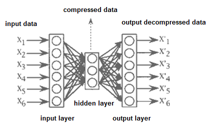
Figure 2: Scheme of feed-forward neural network for lossy compression

The compression process consist of two main steps. First, the neural network must be trained to adjust weights, that were randomly selected. With those adjusted weights, the result hidden layer is generated. Input image is usually divided into N dimensional vectors. Those vectors are inputs of an neural network. In the compression step, each of N vector is replaced with M values from the hidden layer. One of the main disadvantages is the compression time. Adjusting weights is a slow process. An improvement of a compression speed was proposed in [31]. Initialized weights are not randomly selected, but they are chose as a result from genetic algorithm. Later, weights are improved with traditional back-propagation. Another approach is to improve back-propagation [14] or use a different training method. One possibility is theLevenberg-Marquardt method as proposed in [26]. Use of this method can be significant speed up for the networks with only one hidden layer ([44], [45]). Improvement in compression ratio and quality can be achieved witch histogram equalization [12].

4.2.2 Contours

The main idea is to compress only important parts of an image. The reconstructed image is than very similar to a vector graphics representation of bitmap image. Level of details in image depends on the compression ratio. Those method achieves a very good results for a cartoon based images, where contours are the most important parts. Areas are usually filled with not much detail. Such method was described by [20]. Same author in [19] further improved method and test it also on natural images. They used the Marr-Hidreth detector to obtain image edges (but any other edge detector can be used as well). Obtained edges are filtered to preserve only those, that are important. Result is binary image, losslessly encoded with JBIG algorithm. For color compression is used quantization scheme. Colors from both sides of contours are obtained and quantized. Result is again losslessly saved with PAQ algorithm. Its computational cost is balanced with compression ratio. For decompression, quantized colors are interpolated with homogeneous diffusion. For targeting cartoon images, quality is very good (no artefacts like in transform based methods), but for natural ones, the quality is worse. The method for natural images was proposed in [37]. Edges are not obtained with an edge detector, but with a method similar to marching squares. Its advantage is, that we can obtain enclosed areas. For every brightness value in the image, set of contours is obtained. According to the threshold level, some of them are omitted and rest is stored with its brightness value. Level of detail can be also controlled. One possibility is to store only those contours that are longer than a certain threshold. Second possibility is to simplification using e.g. the Ramer–Douglas–Peucker algorithm [10]. A contour can be later stored by its significant points or using chain code. Chain codes can be more compact.

4.2.3 SVD

With an image representation as a matrix in a mathematical sort of view, work methods based on SVD (Singular Value Decomposition), first introduced in [4]. Image is decomposed to three matrices (equations 3 and 4).

$$A=U\Sigma V^{T}$$ (3)

$$A=\left[u_{1}.....u_{n}\right]\left[\begin{array}[]{ccccc}\sigma_{1}\\ &.\\ &&.\\ &&&.\\ &&&&\sigma_{n}\end{array}\right]\left[\begin{array}[]{c}v_{1}\\ .\\ .\\ .\\ v_{n}\end{array}\right]$$ (4)

There is no compression at this point, since we enlarged original 8bit values to floating point numbers. Matrix $\sum$ is diagonal, U and V members are vectors ($u_{n}$ with size M and $v_{n}$ N for MxN image). Compression can be achieved by removing columns and rows from matrices, as illustrated on Figure 3.

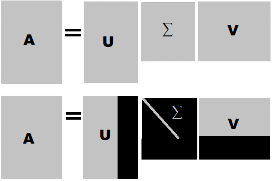
Figure 3: Process of SVD compression. First line are full SVD matrices. Second line represent compression form after removing unnecessary values in black areas.

Main disadvantage is a speed of the compression. Quality is also lower with comparison to DCT. SVD method was improved for example in [32], where image is preprocessed before SVD step. In this article can also be found comparison of SVD with KLT transform. SVD variation for color images can be found in [1].

4.2.4 Other

There are other methods that were researched. One of such approaches is based on a spline interpolation of image [24]. Only a few pixels of image are taken and those are interpreted with a cubic spline. Control points of a spline are selected to minimize overall error of approximation. One of possible approach can be bisection method. If error of section is lower than selected threshold, no further division occurs. Non-control points are set as empty value and image is stored. In a reconstruction, missing values are computed from a cubic spline interpolation. The proposed technique is tested on RGB images, but same approach also works in grayscale.

Quadtree based structures can also be used for image compression. One of the first algorithms with this approach was presented in [41]. In [15] improved algorithm was used. Quadtree leaf is further divided according to its analysis (high or low detail image block). Analysis is done using quantized histogram of difference block (mean is subtracted from each block value). Peaks bigger than threshold are found in histogram. Number of peaks is used as block classificator. If block is low-detailed, its mean value is stored, otherwise division continue. If block is 4x4, no further division is performed. Block is stored with binary mask instead. The best mask is chosen from predefined patterns.

Dictionary based methods are well known in a lossless image compression (PNG, GIF). Its modification for lossy compressions was proposed in [11]. Basic ideas is to create longer sequences of the same value using quantization. This can be best shown on simple example. Assuming data sequence 159, 160, 159, 157, 170, we quantize this and obtain 159, 159, 159, 159, 170. This can be better compressed using dictionary method. Second option is to used similarity of blocks. If difference error of two blocks is lower than threshold, block can be replaced one with another. That also improves compression. Dictionary based methods are similar to near-lossless ones and can also be used that way.

5 Comparison

In this section, comparison of earlier discussed methods is conducted. Compressed size is expressed in bits per pixel (bpp). Using this metric is more readable, because it is image dimension independent. This value can be very easily computed using equation 5.

$$bpp=\frac{8}{M\cdot N}\cdot size$$ (5)

$M$and $N$ refer to image dimensions, $size$ is size of compressed image in bytes.

Besides compressed size, visual quality of reconstructed image is very important for lossy compressions. As one of standards in this area is PSNR (Peak signal-to-noise ratio). We can found results using this metric in almost every article dealing with lossy image compression. PSNR is computed based on MSE (Mean Square Error). Full equation is shown in 6.

$$MSE=\frac{1}{M\cdot N}\sum_{i=0}^{M}\sum_{j=0}^{N}||I(i,j)-K(i,j)||^{2}$$

$$PSNR=10\cdot log\frac{255^{2}}{MSE}$$ (6)

$M$and $N$ refer to image dimensions, $I(i,j)$ signifies original pixel intensity at location (i,j) and $K(i,j)$ denotes pixel intensity in reconstructed image.

5.1 Lossless compression

Lossless compression was tested on the image set from Figure 4 (their histograms can be found on Figure 5). Results are taken directly from cited articles and compared to each other. Same methods can be often found in different articles for comparison with their methods. We collect all those data and created summarized table. Sometimes, tests for certain image were not provided, in that case value “$-$” is used. Collected results can be seen in Table 1.

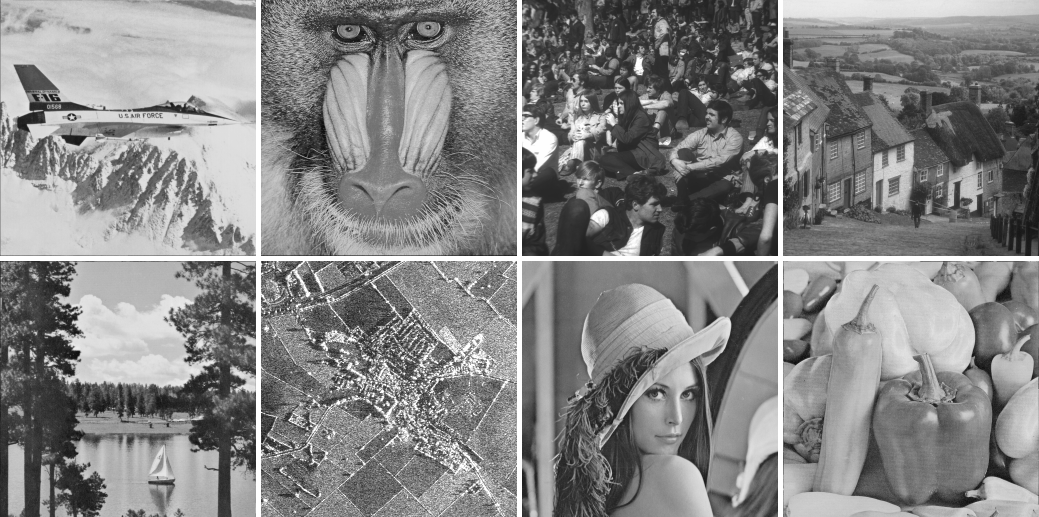
Figure 4: Test images used in Table 1. From left to right: Airplane, Crowd, Baboon (or Mandrill), Goldhill, Lake, Landsat, Lenna, Peppers.

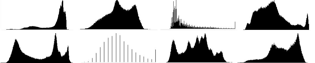
Figure 5: Histograms of test images from Figure 4. The order of images is same as in Figure 4.

	[9]	[35]	[46]	[23]	[43]	[29]	[27]	[6]	[16]	[28]	[5]	[2]	[18]
Airplane	5.69	3.97	3.51	3.62	3.78	3.98	3.92	4.03	3.90	-	4.23	4.39	-
Baboon	7.30	6.16	5.74	5.65	6.04	6.11	5.93	5.98	6.04	5.08	6.88	-	3.60
Crowd	5.84	-	3.76	4.03	3.91	4.19	-	-	-	-	-	-	-
Goldhill	6.66	4.63	4.63	4.66	4.71	4.84	4.54	-	4.48	-	4.73	5.08	4.30
Lake	6.84	-	4.90	4.93	4.92	5.90	-	-	-	8.53	5.37	5.35	-
Landsat	3.98	-	3.99	4.04	7.17	7.36	-	-	-	-	-	-	-
Lenna	6.84	4.18	4.11	4.05	4.23	4.31	4.15	4.44	4.24	5.07	4.54	5.09	3.80
Peppers	5.34	4.68	4.20	4.16	4.85	4.93	4.55	4.59	4.51	-	4.81	5.30	2.80
AVG	6.06	4.91	4.50	4.54	4.95	5.20	4.80	4.76	4.63	4.42	5.21	5.04	3.63

Table 1: Lossless compression sizes in bpp for standard set of images with resolution 512x512. PNG is [9], CALIC is [46], JPEG-LS is [43] and JPEG2000 is [29]. Other methods are not acknowledged as standards.

Even though there are some missing data, we can see the overall compression performance. The worst overall result came from the oldest tested algorithm, PNG ([9]). The only image, where this method is competitive, is landsat. Its because of its character - image has only 20 brightness values (see Figure 5). On the other hand, the best result is from the newest one, that is using DWT transform ([18]).

There can also be seen some kind of dependency between compressed size and histogram. If we look at image of Airplane and Crowd, they have very similar histograms (only reversed). Their compression ratios are also very similar for all tested methods.

5.2 Lossy compression

For the lossy compression test, standard image, that can be found in practically every publication, is Lenna (mostly in resolution 256x256). Our tests will be summarized in graph, because of its clarity. In lossless test, there was only one possible result. For lossy compression, we can get different PSNR values for different compressed size. In our tests we used images from Figure 6.

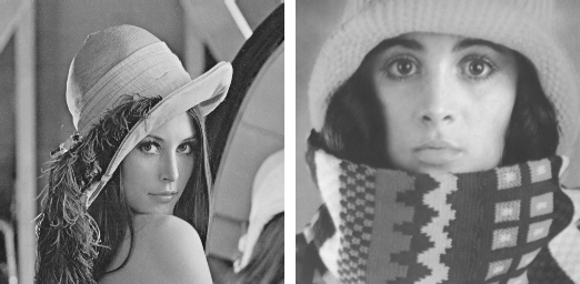
Figure 6: Test images used in Figure 7 and Figure 8. From left to right: Lenna, Trui

First test is using Lenna image in resolution 256x256. Results can be seen on Figure 7. Best result were achieved with JPEG2000 compression, that significantly outperforms other methods. Very similar results were achieved with JPG and both tested quadtree methods ([41] and [15]). For larger compression ratios, neural network from [31] is also competitive. The worst results were, as aspected, achieved with contour based compression ([37]). This method is more suitable for specialized images, mostly cartoon graphic (as was discussed in [19]).

We also added one of near-lossless methods for comparison. That is JPEG-LS, based on [43]. We set different quality loss and simulated classic lossy method. As we can see, for higher bitrates, the quality improves very fast, which is basic of near-lossless method.

We can see some strange behaviour for neural network based compression ([14]). For lower bitrate, we have better PSNR. This effect can be caused by learning problems with neural networks. We have tried to bypass this problem by taking the best results from several independent tests, but as we can see, problem still persist in a lower bitrates.

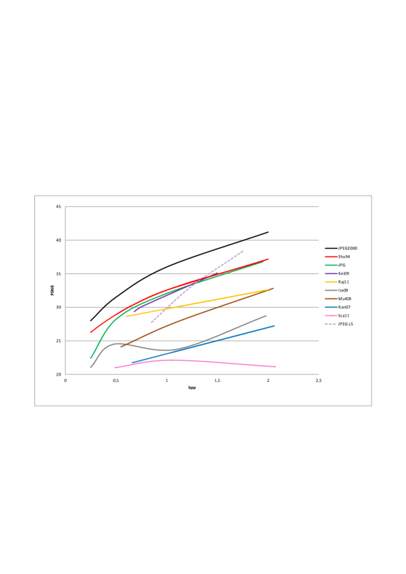
Figure 7: PSNR and compression in bpp for image Lenna in resolution of 256x256. Graph legend is sorted from the best to worst overall method.

Second test is using Trui image in resolution 256x256. Results can be seen on Figure 8. Results for our second image are similar to first one. The best method is again JPEG2000, but this time with lower lead. Improvement for lower bitrates of JPEG2000, [38], provides better results as expected. However, for larger bitrates, quality can be outperformed by JPG. Spline based method [24] provides better results, than for Lenna image. If we look at Trui, we can see the consequence of this behaviour. Trui has more smooth areas, and spline can better describe them. Lenna has more hard edges, were spline is not quite accurate.

Test with near-lossless JPEG-LS (based on [43]) behave similar to one with Lenna image. Only for now, the progress of quality loss is slower. The reason is similar to one, why spline methods works better.

The worst result is, again, achieved with [37].

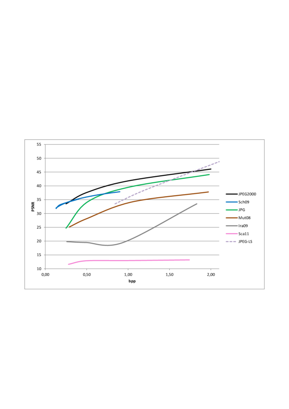
Figure 8: PSNR and compression in bpp for image Trui in resolution of 256x256. Graph legend is sorted from the best to worst overall method.

6 Conclusion

We have discussed and compared various image compression methods. There are many more techniques, that were not covered. The need for a better quality and compression ratio is very important. However, as we can see today, compression techniques commonly used for images are not very modern. The question of compression is much more complicated.

New compression algorithm is just the beginning. Second step, to carry through that method, is much more difficult. We can take simple example from our comparison. Prediction based method (JPEG-LS) has been developed in year 2000 and it is recognized as industrial standard. It outperforms PNG and lossless JPEG2000 (in both, quality and speed). And how common can we found images in this format?

References

- [1] Bethany Adams and Nina Manual. Using the singular value decomposition particularly for the compression of color images, 2005.
- [2] A. Alarabeyyat, S. Al-Hashemi, T. Khdour, M. Hjouj Btoush, S. Bani-Ahmad, R. Al-Hashemi, and S. Bani-Ahmad. Lossless image compression technique using combination methods. Journal of Software Engineering and Applications, 05(10):752–763, 2012.
- [3] Florin Alexa, Vasile Gui, Catalin Caleanu, and Corina Botoca. Lossless data compression using neural networks. In Proceedings of the 7th conference on Circuits, systems, electronics, control and signal processing, CSECS’08, pages 128–132, Stevens Point, Wisconsin, USA, 2008. World Scientific and Engineering Academy and Society (WSEAS).
- [4] Harry C. Andrews and III Patterson, C. Singular value decomposition (svd) image coding. Communications, IEEE Transactions on, 24(4):425–432, 1976.
- [5] A. Avramovic and B. Reljin. Gradient edge detection predictor for image lossless compression. In ELMAR, 2010 PROCEEDINGS, pages 131–134, 2010.
- [6] Tahar Brahimi, Ali Melit, and Fouad Khelifi. An improved {SPIHT} algorithm for lossless image coding. Digital Signal Processing, 19(2):220 – 228, 2009.
- [7] Macarie Breazu, Antoniu Pitic, Daniel Volovici, and Remus Brad. Near-lossless lzw image compression. In SINTES 10 Conference, Caiova, Romania, 2003.
- [8] R.J. Cintra and F.M. Bayer. A dct approximation for image compression. Signal Processing Letters, IEEE, 18(10):579–582, 2011.
- [9] Lee Daniel Crocker. PNG: The Portable Network Graphic format. Dr. Dobb’s Journal, 20(7):36–44, Jully 1995.
- [10] DAVID H DOUGLAS and THOMAS K PEUCKER. Algorithms for the reduction of the number of points required to represent a digitized line or its caricature. Cartographica: The International Journal for Geographic Information and Geovisualization, 10:112–122, 1973.
- [11] Gabriela Dudek, Przemyslaw Borys, and Zbigniew J. Grzywna. Lossy dictionary-based image compression method. Image and Vision Computing, 25(6):883 – 889, 2007.
- [12] S. Anna Durai and E. Anna Saro. Image compression with back-propagation neural network using cumulative distribution function, September 2006.
- [13] P.J.S.G. Ferreira and A.J. Pinho. Why does histogram packing improve lossless compression rates? Signal Processing Letters, IEEE, 9(8):259–261, 2002.
- [14] Saeid Iranmanesh. A differential adaptive learning rate method for back-propagation neural networks. In Proceedings of the 10th WSEAS international conference on Neural networks, NN’09, pages 30–34, Stevens Point, Wisconsin, USA, 2009. World Scientific and Engineering Academy and Society (WSEAS).
- [15] F. Keissarian. A new quadtree-based image compression technique using pattern matching algorithm. International Conference on Computational & Experimental Engineering and Sciences, 12:137–144, 2009.
- [16] H. Kikuchi, K. Funahashi, and S. Muramatsu. Simple bit-plane coding for lossless image compression and extended functionalities. In Picture Coding Symposium, 2009. PCS 2009, pages 1–4, 2009.
- [17] Juan Ignacio Larrauri. A new algorithm for lossless compression applied to two-dimensional static images. In Proceedings of the 6th international conference on Communications and Information Technology, and Proceedings of the 3rd World conference on Education and Educational Technologies, WORLD-EDU’12/CIT’12, pages 56–60, Stevens Point, Wisconsin, USA, 2012. World Scientific and Engineering Academy and Society (WSEAS).
- [18] Jia Li. An improved wavelet image lossless compression algorithm. Optik - International Journal for Light and Electron Optics, 124(11):1041 – 1044, 2013.
- [19] Markus Mainberger, Andrés Bruhn, Joachim Weickert, and SÞren Forchhammer. Edge-based compression of cartoon-like images with homogeneous diffusion. Pattern Recognition, 44(9):1859 – 1873, 2011. <ce:title>Computer Analysis of Images and Patterns</ce:title>.
- [20] Markus Mainberger and Joachim Weickert. Edge-based image compression with homogeneous diffusion. In Xiaoyi Jiang and Nicolai Petkov, editors, Computer Analysis of Images and Patterns, volume 5702 of Lecture Notes in Computer Science, pages 476–483. Springer Berlin Heidelberg, 2009.
- [21] A.S. Mamatha and V. Singh. Near lossless image compression system. In Microelectronics and Electronics (PrimeAsia), 2012 Asia Pacific Conference on Postgraduate Research in, pages 35–41, 2012.
- [22] T. Meyyappan, S.M. Thamarai, and N.M. Jeya Nachiaban. A new method for lossless image compression using recursive crack coding. In Dhinaharan Nagamalai, Eric Renault, and Murugan Dhanuskodi, editors, Advances in Digital Image Processing and Information Technology, volume 205 of Communications in Computer and Information Science, pages 128–135. Springer Berlin Heidelberg, 2011.
- [23] G. Motta, J.A. Storer, and B. Carpentieri. Lossless image coding via adaptive linear prediction and classification. Proceedings of the IEEE, 88(11):1790–1796, 2000.
- [24] R. Muthaian, K. NeelaKantan, Sharma V., and Arora A. Image compression and reconstruction using cubic spline interpolation technique. American Journal of Applied Sciences, 5:1562–1564, November 2008.
- [25] E. Nasr-Esfahani, S. Samavi, N. Karimi, and S. Shirani. Near-lossless image compression based on maximization of run length sequences. In Image Processing, 2007. ICIP 2007. IEEE International Conference on, volume 4, pages IV – 177–IV – 180, 2007.
- [26] N. Sreekumar P. Karthikeyan. A study on image compression with neural networks using modified levenberg maruardt method. Global Journal of Computer Science and Technology, 11, March 2011.
- [27] H. Pan, W. C Siu, and N.F. Law. Lossless image compression using binary wavelet transform. Image Processing, IET, 1(4):353–362, 2007.
- [28] E. Puthooran, R.S. Anand, and S. Mukherjee. Lossless image compression using bpnn predictor with contextual error feedback. In Multimedia, Signal Processing and Communication Technologies (IMPACT), 2011 International Conference on, pages 145–148, 2011.
- [29] Majid Rabbani and Rajan Joshi. An overview of the {JPEG} 2000 still image compression standard. Signal Processing: Image Communication, 17(1):3 – 48, 2002. <ce:title>JPEG 2000</ce:title>.
- [30] V.N.P. Raj and T. Venkateswarlu. A novel approach to medical image compression using sequential 3d dct. In Conference on Computational Intelligence and Multimedia Applications, 2007. International Conference on, volume 3, pages 146–152, 2007.
- [31] G G Rajput and Vrinda Shivashetty. Modeling of neural image compression using ga and bp : a comparative approach. IJACSA - International Journal of Advanced Computer Science and Applications, (Special Issue):26–34, 2011.
- [32] Abhiram Ranade, Srikanth S. Mahabalarao, and Satyen Kale. A variation on svd based image compression. Image and Vision Computing, 25(6):771 – 777, 2007.
- [33] Kamisetty Ramamohan Rao and Pat Yip, editors. The Transform and Data Compression Handbook. CRC Press, Inc., Boca Raton, FL, USA, 2000.
- [34] Vinay Rawat, Ravindra Singh, Mayank Pawar, and Raj Mishra. Lossless gray image compression using logic minimization. Recent Research in Science and Technology, 4(1), 2012.
- [35] A. Said and W.A. Pearlman. A new, fast, and efficient image codec based on set partitioning in hierarchical trees. Circuits and Systems for Video Technology, IEEE Transactions on, 6(3):243–250, 1996.
- [36] David Salomon. Data Compression: The Complete Reference. Second edition, 2000.
- [37] G. Scarmana. A contour-based approach to image compression. In Digital Image Computing Techniques and Applications (DICTA), 2011 International Conference on, pages 186–190, 2011.
- [38] Christian Schmaltz, Joachim Weickert, and Andres Bruhn. Beating the quality of jpeg 2000 with anisotropic diffusion. In Joachim Denzler, Gunther Notni, and Herbert Susse, editors, Pattern Recognition, volume 5748 of Lecture Notes in Computer Science, pages 452–461. Springer Berlin Heidelberg, 2009.
- [39] R.K. Senapati, U.C. Pati, and K.K. Mahapatra. A low complexity orthogonal 8x8 transform matrix for fast image compression. In India Conference (INDICON), 2010 Annual IEEE, pages 1–4, 2010.
- [40] J.M. Shapiro. Embedded image coding using zerotrees of wavelet coefficients. Signal Processing, IEEE Transactions on, 41(12):3445–3462, 1993.
- [41] E. Shusterman and M. Feder. Image compression via improved quadtree decomposition algorithms. Image Processing, IEEE Transactions on, 3(2):207–215, 1994.
- [42] G.K. Wallace. The jpeg still picture compression standard. Consumer Electronics, IEEE Transactions on, 38(1):xviii–xxxiv, 1992.
- [43] M.J. Weinberger, G. Seroussi, and G. Sapiro. The loco-i lossless image compression algorithm: principles and standardization into jpeg-ls. Image Processing, IEEE Transactions on, 9(8):1309–1324, 2000.
- [44] B.M. Wilamowski, Yixin Chen, and A. Malinowski. Efficient algorithm for training neural networks with one hidden layer. In Neural Networks, 1999. IJCNN ’99. International Joint Conference on, volume 3, pages 1725–1728 vol.3, 1999.
- [45] B.M. Wilamowski and Hao Yu. Improved computation for levenberg-marquardt training. Neural Networks, IEEE Transactions on, 21(6):930–937, 2010.
- [46] Xiaolin Wu and N. Memon. Calic-a context based adaptive lossless image codec. In Acoustics, Speech, and Signal Processing, 1996. ICASSP-96. Conference Proceedings., 1996 IEEE International Conference on, volume 4, pages 1890–1893 vol. 4, 1996.
- [47] Daoqiang Zhang and Songcan Chen. Fast image compression using matrix k-l transform. Neurocomput., 68:258–266, October 2005.
- [48] J. Ziv and A. Lempel. A universal algorithm for sequential data compression. Information Theory, IEEE Transactions on, 23(3):337–343, 1977.