Giant and pigmy dipole resonances in ⁴He, ^16,22O, and ⁴⁰Ca from chiral nucleon-nucleon interactions

Abstract

We combine the coupled-cluster method and the Lorentz integral transform for the computation of inelastic reactions into the continuum. We show that the bound–state–like equation characterizing the Lorentz integral transform method can be reformulated based on extensions of the coupled-cluster equation-of-motion method, and we discuss strategies for viable numerical solutions. Starting from a chiral nucleon-nucleon interaction at next-to-next-to-next-to-leading order, we compute the giant dipole resonances of ⁴He, ^16,22O and ⁴⁰Ca, truncating the coupled-cluster equation-of-motion method at the two-particle-two-hole excitation level. Within this scheme, we find a low-lying $E1$ strength in the neutron-rich ²²O nucleus, which compares fairly well with data from [Leistenschneider et al. Phys. Rev. Lett. 86, 5442 (2001)]. We also compute the electric dipole polariziability in ⁴⁰Ca. Deficiencies of the employed Hamiltonian lead to overbinding, too small charge radii and a too small electric dipole polarizability in ⁴⁰Ca.

I Introduction

The inelastic response of an $A$-body system due to its interaction with perturbative probes is a basic property in quantum physics. It contains important information about the dynamical structure of the system. For example, in the history of nuclear physics the study of photonuclear reactions lead to the discovery of giant dipole resonances (GDR) Baldwin and Klaiber (1947), originally interpreted as a collective motion of protons against neutrons. For neutron-rich nuclei far from the valley of stability, such collective modes exhibit a fragmentation with low-lying strength, also called pigmy dipole resonances (see, e.g., Ref. Leistenschneider et al. (2001)), typically interpreted as due to the oscillation of the excess neutrons against a core made by all other nucleons.

Recently, progress was made in computing properties of medium mass and some heavy nuclei from first-principles using a variety of methods such as the coupled-cluster method Kümmel et al. (1978); Bishop (1991); Hagen et al. (2013), in-medium similarity-renormalization-group method Tsukiyama et al. (2011); Hergert et al. (2013), the self-consistent Green’s function method Dickhoff and Barbieri (2004); Somà et al. (2013), and lattice effective field theory Lähde et al. (2014). Although most of these methods focused on bound-state properties of nuclei, there has been progress in describing physics of unbound nuclear states and elastic neutron/proton scattering with application to the neutron rich helium Hagen et al. (2007) and calcium isotopes Hagen et al. (2012a); Hagen and Michel (2012); Hagen et al. (2013). However, these continuum calculations are currently limited to states that are of single-particle like structure and below multi-nucleon breakup thresholds.

The microscopic calculation of final–state continuum wave functions of nuclei in the medium-mass regime constitutes still an open theoretical problem. This is due to the fact that at a given continuum energy the wave function of the system has many different components (channels) corresponding to all its partitions into different fragments of various sizes. Working in configuration space one has to find the solution of the many–body Schrödinger equation with the proper boundary conditions in all channels. The implementation of the boundary conditions constitutes the main obstacle to the practical solution of the problem. In momentum space the difficulty translates essentially into the proliferation with $A$ of the Yakubovsky equations as well as into the complicated treatment of the poles of the resolvents. For example, the difficulties in dealing with the three-body break-up channel for ⁴He have been overcome only very recently Deltuva and Fonseca (2012).

The Lorentz integral transform (LIT) method Efros et al. (1994) allows to avoid the complications of a continuum calculation, because it reduces the difficulties to those typical of a bound–state problem, where the boundary conditions are much easier to implement. The LIT method has been applied to systems with $A\leq 7$ using the Faddeev method Martinelli et al. (1995), the correlated hyperspherical-harmonics method Efros et al. (1997a, b, c, 1998, 2000), the EIHH method Bacca et al. (2002, 2004a, 2004b); Gazit et al. (2006a) or the NCSM Stetcu et al. (2007); Quaglioni and Navrátil (2007). All those methods, however, have been introduced for dealing with typical few–body systems and cannot be easily extended to medium–heavy nuclei. Therefore it is desirable to formulate the LIT method in the framework of other many–body methods. In the present work we present such a formulation for the coupled–cluster (CC) method Coester (1958); Coester and Kümmel (1960); Čížek (1966, 2007); Čížek and Paldus (1971); Kümmel et al. (1978), which is a very efficient bound-state technique applied with success on several medium–mass and a few heavy nuclei Dean and Hjorth-Jensen (2004); Kowalski et al. (2004); Gour et al. (2006); Hagen et al. (2008, 2010, 2012b, 2012a); Roth et al. (2012); Binder et al. (2013, 2014), and see Hagen et al. (2014) for a recent review. First pioneering calculations of the GDR in ¹⁶O obtained by combining the LIT with CC theory have been recently reported in a Letter Bacca et al. (2013). In this paper, we will explain the details of the approach and display comprehensive results on ⁴He, ¹⁶O, and new results on the neutron-rich nucleus of ²²O and on the heavier nucleus of ⁴⁰Ca.

The paper is organized as follows. In Section II a short review of the LIT method is presented. In Section III we formulate it in the framework of CC theory and discuss two possible strategies to solve the resulting equations. In Section IV we validate this method on ⁴He by benchmarking it against converged EIHH calculations. In Sections V, VI and VII we address the dipole response function of ¹⁶O, ²²O and ⁴⁰Ca, respectively. Finally, in Section VIII we draw our conclusions.

II The LIT method - a short review

In order to determine cross sections due to external perturbative probes one has to calculate various dynamical structure functions such as

$$S_{\alpha\beta}(\omega,q)=$$ (1)

$$\sum_{n}\langle 0|{\hat{\Theta}}^{\dagger}_{\alpha}(q)|{n}\rangle\langle{n}|{\hat{\Theta}}_{\beta}(q)|0\rangle\delta(E_{n}-E_{0}-\omega)\>\mbox{.}$$

Here $\omega$ and $q$ are energy and momentum transfer of the external probe, $|0\rangle$ and $|{n}\rangle$ denote ground and final state wave functions of the considered system with energies $E_{0}$ and $E_{n}$, respectively, while ${\hat{\Theta}}_{\alpha}$ denotes excitation operators inducing transitions labeled by $\alpha$. The $\sum_{n}$ indicates both the sum over discrete state and an integration over continuum Hamiltonian eigenstates.

For simplicity let us assume that ${\hat{\Theta}}_{\alpha}(q)={\hat{\Theta}}_{\beta}(q)={\hat{\Theta}}$ and consider the following inclusive structure function (also called response function)

$$S(\omega)=\sum_{n}\langle 0|{\hat{\Theta}}^{\dagger}|{n}\rangle\langle{n}|{\hat{\Theta}}|0\rangle\delta(E_{n}-E_{0}-\omega)\>\mbox{.}$$ (2)

For few or many–body reactions with mass number $A>2$ one very often faces the problem that $S(\omega)$ cannot be calculated exactly, since the microscopic calculation of $|{n}\rangle$ is too complicated, due to the necessity to solve the many-body scattering problem. However, via the LIT approach the problem can be reformulated in such a way that the knowledge of $|{n}\rangle$ is not necessary Efros et al. (1994). To this end the integral transform of the dynamical response function with a Lorentz kernel (LIT) is introduced

$${L}(\omega_{0},\Gamma)=\frac{\Gamma}{\pi}\int d\omega\frac{S(\omega)}{(\omega-\omega_{0})^{2}+\Gamma^{2}}\>\mbox{,}$$ (3)

where $\Gamma>0$. The LIT method proceeds in two steps. First ${L}(\omega_{0},\Gamma)$ is computed in a direct way, which does not require the knowledge of $S(\omega)$, and then in a second step the dynamical function is obtained from an inversion of the LIT Efros et al. (1999); Andreasi, D. et al. (2005).

The function ${L}(\omega_{0},\Gamma)$ can be calculated directly starting from the definition in Eq. (3), substituting the expression in (2) for $S(\omega)$, and using the completeness relation of the Hamiltonian eigenstates,

$$\sum_{n}|{n}\rangle\langle{n}|=1\>\mbox{.}$$ (4)

Thus,

$${L}(\omega_{0},\Gamma)=\frac{\Gamma}{\pi}\,\times$$ (5)

$$\langle 0|{\hat{\Theta}}^{\dagger}\frac{1}{\hat{H}-E_{0}-\omega_{0}+i\Gamma}\frac{1}{\hat{H}-E_{0}-\omega_{0}-i\Gamma}\hat{\Theta}|0\rangle\>\mbox{.}$$

The solutions $|\widetilde{\Psi}\rangle$ of the equation

$$(\hat{H}-z)|\widetilde{\Psi}\rangle=\hat{\Theta}|0\rangle$$ (6)

for different values of $\omega_{0}$ and $\Gamma$ lead directly to the transform

$${L}(z)=\frac{\Gamma}{\pi}\langle\widetilde{\Psi}|\widetilde{\Psi}\rangle\>\mbox{.}$$ (7)

Here we introduced the quantity $z=E_{0}+\omega_{0}+i\Gamma$. Since ${L}(z)$ is finite the solution $|\widetilde{\Psi}\rangle$ of Eq. (6) has the same asymptotic boundary conditions as a bound–state. Moreover the solution is unique. In fact if there were two solutions $|\widetilde{\Psi}_{1}\rangle$ and $|\widetilde{\Psi}_{2}\rangle$, the hermiticity of $\hat{H}$, ensures that the homogeneous equation

$$(\hat{H}-z)(|\widetilde{\Psi}_{1}\rangle-|\widetilde{\Psi}_{2}\rangle)=0$$ (8)

has only the trivial solution $(|\widetilde{\Psi}_{1}\rangle-|\widetilde{\Psi}_{2}\rangle)=0$.

From the inversion of the calculated ${L}(\omega_{0},\Gamma)$ one obtains the dynamical function $S(\omega)$. The LIT method leads to an exact response function as shown in benchmarks with other methods for two- and three-body systems Piana and Leidemann (2000); Golak et al. (2002). In the reviews Efros et al. (2007a); Bacca and Pastore (2014) the interested reader can find more details on the LIT method, on the generalizations to exclusive and hadronic processes as well as its application to various electro-weak interactions with light nuclei.

III The LIT in Coupled–Cluster Theory

In coupled-cluster theory we work with the similarity transformed Hamiltonian

$$\overline{H}=\exp(-T)\hat{H}_{N}\exp(T).$$ (9)

Here $H_{N}$ is normal-ordered with respect to a chosen uncorrelated reference state $|\Phi_{0}\rangle$, which is typically the Hartree-Fock state. Correlations are introduced through the cluster operator $T$ which is a linear combination of particle-hole ($ph$) excitation operators, i.e. $T=T_{1}+T_{2}+\ldots$, with the $1p$-$1h$ excitation operator $T_{1}$, the $2p$-$2h$ excitation operator $T_{2}$, and so on. The similarity transformed Hamiltonian (9) is non-Hermitian and has left- and right eigenstates which constitute a complete bi-orthogonal set according to

$$\langle{n}_{L}|{n^{\prime}}_{R}\rangle=\delta_{n,n^{\prime}},\>\>\>\sum_{n}|{n}_{R}\rangle\langle{n}_{L}|=1\,.$$ (10)

We note that the right ground-state is nothing but the reference state, i.e. $|0_{R}\rangle=|\Phi_{0}\rangle$, while the corresponding left ground-state is given by $\langle 0_{L}|=\langle\Phi_{0}|(1+\Lambda)$. Here $\Lambda$ is a linear combination of particle-hole de-excitation operators, see e.g. Bartlett and Musiał (2007).

Using the left and right eigenstates we can define the response function corresponding to the similarity-transformed Hamiltonian $\overline{H}$ analogous to Eq. (2)

$$S(\omega)=\sum_{n}\langle 0_{L}|\overline{\Theta^{\dagger}}|{n}_{R}\rangle\langle{n}_{L}|\overline{\Theta}|0_{R}\rangle\delta(E_{n}-E_{0}-\omega).$$ (11)

The similarity-transformed excitation operators

$$\overline{\Theta}=\exp(-T)\hat{\Theta}\exp(T),\>\>\overline{\Theta^{\dagger}}=\exp(-T)\hat{\Theta}^{\dagger}\exp(T)$$ (12)

enters in Eq. (11). The Baker-Campbell-Hausdorff expansion of $\overline{\Theta}$ terminates exactly at doubly nested commutators in the case of a one-body operator and at quadruply nested commutators in the case of a two-body operator (see, for example, Shavitt and Bartlett (2009) for more details). Substituting Eq. (11) in Eq. (3) and using the completeness relation (10), one obtains

$${L}(\omega_{0},\Gamma)=\frac{\Gamma}{\pi}\,\langle 0_{L}|{\overline{\Theta^{\dagger}}}\frac{1}{\overline{H}-z^{*}}\frac{1}{\overline{H}-z}\overline{\Theta}|0_{R}\rangle,$$ (13)

with $z=E_{0}+\omega_{0}+i\Gamma$, and in analogy with Eq. (7) one has

$${L}(z)\equiv\frac{\Gamma}{\pi}\,\langle\widetilde{\Psi}_{L}(z^{*})|\widetilde{\Psi}_{R}(z)\rangle\,.$$ (14)

Here $\langle\widetilde{\Psi}_{L}|$ and $|\widetilde{\Psi}_{R}\rangle$ satisfy the equations

$$(\overline{H}-z)|\widetilde{\Psi}_{R}(z)\rangle = \overline{\Theta}|0_{R}\rangle$$ (15)

$$\langle\widetilde{\Psi}_{L}(z^{*})|(\overline{H}-z^{*}) = \langle 0_{L}|\overline{\Theta^{\dagger}}\,.$$ (16)

Since $L(z)$ is finite, $|\widetilde{\Psi}_{R}(z)\rangle$ and $\langle\widetilde{\Psi}_{L}(z^{*})|$ must have bound-state like boundary conditions.

Eq. (13) can also be written as

$${L}(z)=-\frac{1}{2\pi}{\rm Im}\left\{\langle 0_{L}|{\overline{\Theta^{\dagger}}}\left(\frac{1}{\overline{H}-z^{*}}-\frac{1}{\overline{H}-z}\right)\overline{\Theta}|0_{R}\rangle\right\},$$ (17)

or as

$${L}(z)=-\frac{1}{2\pi}{\rm Im}\left\{\langle\widetilde{\Psi}_{L}(z^{*})|\overline{\Theta}|0_{R}\rangle-\langle 0_{L}|\overline{\Theta^{\dagger}}|\widetilde{\Psi}_{R}(z)\rangle\right\}\,.$$ (18)

One can also write $L(z)$ in function of $|\widetilde{\Psi}_{R}(z)\rangle$ only, or of $\langle\widetilde{\Psi}_{L}(z^{*})|$ only, as

$${L}(z)=-\frac{1}{2\pi}{\rm Im}\left\{\langle 0_{L}|\overline{\Theta^{\dagger}}\left(|\widetilde{\Psi}_{R}(z^{*})\rangle-|\widetilde{\Psi}_{R}(z)\rangle\right)\right\}$$ (19)

$${L}(z)=-\frac{1}{2\pi}{\rm Im}\left\{\left(\langle\widetilde{\Psi}_{L}(z^{*})|-\langle\widetilde{\Psi}_{L}(z)|\right)\overline{\Theta}|0_{R}\rangle\right\}\,.$$ (20)

Within the coupled–cluster theory, equations (15) and (16), to which we shall refer as the Lorentz-Integral-Transform Coupled-Cluster (LIT-CC) equations, are equivalent to Eq. (8) introduced in the previous Section. They are the key equations to solve to calculate $L(z)$ via either Eq. (14), or any of Eqs. (17)–(20). It is important to remark that in deriving Eqs. (14), (17)–(20) no approximation has been made.

III.1 Solving the LIT-CC equations

As we have seen in the previous Section, being able to solve Eqs. (15) and/or (16) to sufficient accuracy is the key for the success of the method. To solve the LIT-CC equations one may proceed in a way analogous to what is done in the equation-of-motion coupled-cluster method for excited states  Stanton and Bartlett (1993). We therefore write the wave function $|\widetilde{\Psi}_{R}(z)\rangle$ in the form,

$$|\widetilde{\Psi}_{R}(z)\rangle = {\cal R}(z)|\Phi_{0}\rangle\equiv\left(r_{0}(z)+\sum_{ia}r_{i}^{{a}}(z)\hat{c}^{\dagger}_{{a}}\hat{c}_{{i}}+\right.$$ (21)

$$+ \left.\frac{1}{4}\sum_{ijab}r_{ij}^{{ab}}(z)\hat{c}^{\dagger}_{a}\hat{c}^{\dagger}_{b}\hat{c}_{j}\hat{c}_{i}+\ldots\right)|\Phi_{0}\rangle\;,$$

and analogously for $\langle\widetilde{\Psi}_{L}(z^{*})|$ in the form,

$$\langle\widetilde{\Psi}_{L}(z^{*})| = \langle\Phi_{0}|{\mathcal{L}}(z^{*})\equiv\langle\Phi_{0}|\left(l_{0}(z^{*})+\sum_{ia}l_{i}^{{a}}(z^{*})\hat{c}^{\dagger}_{{i}}\hat{c}_{{a}}+\right.$$ (22)

$$+ \left.\frac{1}{4}\sum_{ijab}l_{ij}^{{ab}}(z^{*})\hat{c}^{\dagger}_{i}\hat{c}^{\dagger}_{j}\hat{c}_{b}\hat{c}_{a}+\ldots\right)\;.$$

Substituting $|\widetilde{\Psi}_{R}(z)\rangle$ in Eq. (15) yields

$$(\overline{H}-z){\cal R}(z)|{\Phi}_{0}\rangle=\overline{\Theta}|0_{R}\rangle\;\;,$$ (23)

and similarly for the left equation,

$$\langle\Phi_{0}|{\cal L}(z^{*})(\overline{H}-z^{*})=\langle 0_{L}|\overline{\Theta^{\dagger}}\;\;.$$ (24)

Projecting the last two equations on $n$-particle $n$-hole excited reference states we get a set of linear equations for the amplitude operators ${\mathcal{R}}(z)$ and ${\mathcal{L}}(z^{*})$. These equations are similar to the CC equations-of-motion Stanton and Bartlett (1993) up to the source term on the right–hand–side. As $\overline{H}$ is a scalar under rotatations, the amplitudes ${\mathcal{R}}(z)$ and ${\mathcal{L}}(z^{*})$ exhibit the same symmetries as the excitation operators $\overline{\Theta}$ and $\overline{\Theta^{\dagger}}$, respectively. Once these equations are solved one obtains the LIT as

$${L}(z)=\frac{\Gamma}{\pi}\langle\Phi_{0}|{\mathcal{L}}(z^{*}){\mathcal{R}}(z)|\Phi_{0}\rangle\,,$$ (25)

or

$${L}(z)=-\frac{1}{2\pi}{\rm Im}\left\{\langle\Phi_{0}|{\mathcal{L}}(z^{*})\overline{\Theta}|0_{R}\rangle-\langle 0_{L}|\overline{\Theta^{\dagger}}{\cal R}(z)|\Phi_{0}\rangle\right\}\,,$$ (26)

or

$${L}(z)=-\frac{1}{2\pi}{\rm Im}\left\{\langle 0_{L}|\overline{\Theta}^{\dagger}\left({\cal R}(z^{*})-{\cal R}(z)\right)|\Phi_{0}\rangle\right\}\,,$$ (27)

or

$${L}(z)=-\frac{1}{2\pi}{\rm Im}\left\{\langle\Phi_{0}|({\mathcal{L}}(z^{*})-{\mathcal{L}}(z))\overline{\Theta}|0_{R}\rangle\right\}\,.$$ (28)

We note that $L(z)$ can be computed by solving Eqs. (23)-(24) and any of the Eqs. (25)-(28). These equations provide different, but equivalent, ways of obtaining the LIT. This gives us a valuable tool to check the implamentation of the LIT-CC method. On test examples these different approaches gave identical numerical results.

To obtain $L(z)$ one is required to solve the equations of motion (25)-(28) for every different value of $z$, thus making it not very convenient, especially if the model space size is large. It is thus convenient to reformulate the solutions of these equations by using the Lanczos algorithm.

III.2 The Lanczos method

Here we generalize the Lanczos approach of Ref. Efros et al. (2007b) to non-Hermitian operators and thereby avoid solving Eqs. (23) and (24) for every different value of $z$. Starting, e.g., from Eq. (17) one can write the $L(z)$ in matrix form on the particle-hole basis as

$${L}(z) = -\frac{1}{2\pi}{\rm Im}\left[{\bf S}^{L}\left((\boldsymbol{M}-z^{*})^{-1}\right.\right.$$

$$\left.\left.-(\boldsymbol{M}-z)^{-1}\right)\boldsymbol{S}^{R}\right]\,,$$

where the matrix elements $M_{\alpha,\alpha^{\prime}}$ of $\boldsymbol{M}$ and the components $S^{R}_{\alpha}$ and $S^{L}_{\alpha}$ of the row- and column-vectors $\boldsymbol{S}^{L}$ and $\boldsymbol{S}^{R}$ are given by

$$M_{\alpha,\alpha^{\prime}} = \langle\Phi_{\alpha}|\overline{H}|\Phi_{\alpha^{\prime}}\rangle\,,$$ (30)

$$S^{R}_{\alpha} = \langle\Phi_{\alpha}|\overline{\Theta}|0_{R}\rangle\,,$$ (31)

$$S^{L}_{\alpha} = \langle 0_{L}|\overline{\Theta^{\dagger}}|\Phi_{\alpha}\rangle\,.$$ (32)

The indices $\alpha,\alpha^{\prime}$ run over the $0p$-$0h$,$1p$-$1h$,$2p$-$2h$,$\ldots$ states

$$|\Phi_{0}\rangle,|\Phi_{i}^{a}\rangle=\hat{c}_{a}^{\dagger}\hat{c}_{i}|\Phi_{0}\rangle,|\Phi_{ij}^{ab}\rangle=\hat{c}_{a}^{\dagger}\hat{c}_{b}^{\dagger}\hat{c}_{i}\hat{c}_{j}|\Phi_{0}\rangle,\ldots\;.$$ (33)

Notice that $\boldsymbol{S}^{L}\boldsymbol{S}^{R}=\langle 0_{L}|\overline{\Theta^{\dagger}}\,\overline{\Theta}|0_{R}\rangle=\langle 0|\Theta^{\dagger}\,\Theta|0\rangle$.

At this point we can make use of the Lanczos algorithm to evaluate $L(z)$. However, since the matrix $\boldsymbol{M}$ is nonsymmetric, we use its complex symmetric variant Collum (1995). To this end we define the left and the right vectors

$$\boldsymbol{v}_{0} = \boldsymbol{S}^{R}/\sqrt{\boldsymbol{S}^{L}\boldsymbol{S}^{R}}$$ (34)

$$\boldsymbol{w}_{0} = \boldsymbol{S}^{L}/\sqrt{\boldsymbol{S}^{L}\boldsymbol{S}^{R}}\,.$$ (35)

Equation (III.2) becomes

$${L}(z)=-\frac{1}{2\pi}\rm{Im}\left\{\left[\boldsymbol{S}^{L}\boldsymbol{S}^{R}\right]\right.$$ (36)

$$\left.{\boldsymbol{w}_{0}}\left[(\boldsymbol{M}-z^{*})^{-1}-(\boldsymbol{M}-z)^{-1}\right]\boldsymbol{u}_{0}\right\}\,.$$

One notices that the LIT depends on the matrix element

$$x_{00}\equiv\boldsymbol{w}_{0}(\boldsymbol{M}-z)^{-1}\boldsymbol{u}_{0}\>.$$ (37)

One can calculate $x_{00}$ applying Cramer’s rule to the solution of the linear system

$$\sum_{\beta}(\boldsymbol{M}-z)_{\alpha\beta}x_{\beta 0}=\delta_{\alpha 0}\,,$$ (38)

which arises from the identity

$$(\boldsymbol{M}-z)(\boldsymbol{M}-z)^{-1}=I$$ (39)

on the Lanczos basis $\{\boldsymbol{u}_{i},\boldsymbol{w}_{i}\mbox{,}i=0\mbox{,}\ldots\mbox{,}n-1\}$. In the Lanczos basis $\boldsymbol{M}$ takes on a tridiagonal form

$$\boldsymbol{M}=\left(\begin{array}[]{ccccc}a_{0}&b_{0}&0&0&\cdots\\ b_{0}&a_{1}&b_{1}&0&\cdots\\ 0&b_{1}&a_{2}&b_{2}&\cdots\\ 0&0&b_{2}&a_{3}&\cdots\\ \vdots&\vdots&\vdots&\vdots&\ddots\end{array}\right)\>\mbox{.}$$ (40)

In this way one is able to write $x_{00}$ as a continued fraction containing the Lanczos coefficients $a_{i}$ and $b_{i}$,

$$x_{00}(z)=\frac{1}{a_{0}-z+\frac{b^{2}_{1}}{a_{1}-z+\frac{b^{2}_{2}}{a_{2}-z+b^{2}_{3}\ldots}}}\>,$$ (41)

and thus also the LIT becomes a function of the Lanczos coefficients

$${L}(z)=-\frac{1}{2\pi}{\rm Im}\left\{\left[\boldsymbol{S}^{L}\boldsymbol{S}^{R}\right]\left[x_{00}(z^{*})-x_{00}(z)\right]\right\}\ .$$ (42)

This illustrates that the Lanczos method allows to determine $L(z)$ without inverting the Hamiltonian matrix.

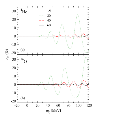
Figure 1: (Color online) The relative convergence of the LIT $L(\omega_{0},\Gamma)$ as a function of the number $N$ of Lanczos steps: ⁴He in panel (a) and ¹⁶O in panel (b). The LIT are calculated for $\Gamma=10$ MeV.

The Lanczos approach outlined above has few important advantages for the LIT method. First of all, the tridiagonalization of ${\bf M}$ has to be done only once regardless of the value of $\omega_{0}$ and $\Gamma$. Moreover, one can usually converge with reasonably few Lanczos vectors (depending on the nucleus and the excitation operator $\Theta$). This is expected since at low values of $\omega_{0}$ the LIT is dominated by the lowest eigenvalues of ${\bf M}$, and for $\omega_{0}\longrightarrow\infty$, $L(z)$ is dominated by the first Lanczos vector.

Figure 1 shows the fast convergence rate (for a dipole operator) by showing the ratio

$$r_{N}(\omega_{0},\Gamma)=[{L}_{N}(\omega_{0},\Gamma)-{L}(\omega_{0},\Gamma)]/{L}(\omega_{0},\Gamma)\times 100\,,$$ (43)

where ${L}_{N}(\omega_{0},\Gamma)$ is the LIT calculated with ${N}$ Lanczos steps and ${L}(\omega_{0},\Gamma)$ is the converged result. The curves are obtained with $\Gamma=10$ MeV. The convergence is indeed very fast and with 60 Lanczos steps one can reach a numerical precision which is below one percent, and about 90 Lanczos vectors are sufficient to reach convergence.

III.3 Removal of spurious states

In this paper, we will apply the LIT-CCSD method to the computation of the dipole response and use the excitation operator $\Theta\equiv\hat{\bf D}$ where $\hat{\bf D}$ is the translationally invariant dipole operator, see Eq. (46) below. The state $\hat{\bf D}|0_{R}\rangle$ is a $J^{\pi}=1^{-}$ state (and similar for the bra state) and therefore has the same quantum numbers as spurious center-of-mass excitations.

The coupled-cluster method employs the intrinsic Hamiltonian

$$H=T-T_{\rm CoM}+V\ .$$ (44)

Here, $T$ is the total kinetic energy, $T_{\rm CoM}$ is the kinetic energy of the center of mass, and $V$ is the translationally invariant potential. For the intrinsic Hamiltonian, coupled-cluster computations of ground and excited states avoid center-of-mass admixtures to a good precision for practical purposes Hagen et al. (2009, 2010). Spurious center-of-mass excitations can be identified as described by Jansen (2013). However, the coupled-cluster wavefunctions are not simply products of an intrinsic wavefunctions and a center-of-mass wavefunction. This is problematic when the Lanczos procedure is applied to the state $\hat{\bf D}|0_{R}\rangle$, because any small admixture of $\hat{\bf D}|0_{R}\rangle$ with a center-of-mass state gets amplified in the Lanczos iteration. As a consequence, the diagonalization of the complex symmetric Lanczos matrix $\boldsymbol{M}$ of Eq. (40) yields a very low-lying (and spurious) $J^{\pi}=1^{-}$ state. In sufficiently large model spaces of about 10 oscillator shells or so, this spurious state is below 1 MeV of excitation energy. The spurious state would be at exactly zero energy if the factorization of the intrinsic and center-of-mass wavefunction were perfect in the coupled-cluster method.

In order to remove spurious states, we follow a procedure which is similar to that used to remove the elastic contributions in electron scattering Bacca et al. (2007). As it was noticed in Efros et al. (2007b), when using any diagonalization method the LIT in Eq. (5) can be expressed as

$$L(z) = \frac{1}{\pi}{\rm Im}\left\{\sum_{\nu}\frac{|\langle\varphi_{\nu}^{N}|\Theta|0\rangle|^{2}}{\epsilon_{\nu}^{N}-z}\right\}$$ (45)

$$= \frac{\Gamma}{\pi}\sum_{\nu}\frac{|\langle\varphi_{\nu}^{N}|\Theta^{\dagger}|0\rangle|^{2}}{(\epsilon_{\nu}^{N}-E_{0}-\omega_{0})^{2}+\Gamma^{2})}\,.$$

Here the $\epsilon_{\nu}^{N}$ and $\varphi_{\nu}^{N}$ are eigenvalues and eigenfunctions of the diagonalized Hamiltonian matrix (the index $N$ reminds us that both quantities depend on the size of the basis). Thus, the LIT is a sum of Lorentzians centered at $\epsilon_{\nu}^{N}$ and of width $\Gamma$. Of course this is also the case when using the Lanczos diagonalization and the similarity transformed Hamiltonian. Therefore, a spurious state $\varphi_{\nu}^{N}$ can be removed by omitting it in the sum in Eq. (45).

IV Validation in ⁴He

By reformulating the LIT approach within the CC theory we have obtained a new method to tackle break-up observables in nuclei. As we have already stressed this method is in principle exact and approximations only enter through truncation of the $T$ operator in the similarity transformations in Eqs. (9) and (12), and through truncation at a given particle-hole excitation level in the excited states $|\tilde{\Psi}_{R}\rangle$ and $\langle\tilde{\Psi}_{L}|$ given in Eqs. (21) and (22). In what follows we will consider an expansion up to two-particle-two-hole excitations in both the cluster amplitude $T$ and the excitation operators $\mathcal{R}$ and $\mathcal{L}$, respectively. This approximation is analogous with the standard equation-of-motion coupled-cluster with singles-and-doubles excitations (EOM-CCSD) method Bartlett and Musiał (2007). In the following we label our approximation of the LIT-CC equations by LIT-CCSD. The computational cost of the LIT-CCSD scheme is the same as that of EOM-CCSD, namely $n_{o}^{2}n_{u}^{4}$ where $n_{o}$ is the number of occupied orbitals and $n_{u}$ is number of un-occupied orbitals. In order to reach model-space sizes large enough to obtain converged results we solve the LIT-CC equations in an angular momentum coupled scheme Hagen et al. (2008, 2010). The EOM-CCSD diagrams and their corresponding angular momentum coupled algebraic expressions can be found in Hagen et al. (2014).

We first want to benchmark this new method with a known solution of the problem. For the mass number $A=4$ extensive studies have been done with the accurate EIHH method Barnea et al. (2001). By comparing EIHH and CC results for ⁴He, where the same interaction and excitation operator are used, we can study the convergence pattern and assess the accuracy of the approximations introduced in the LIT-CCSD scheme.

In all the results shown for this benchmark, and in the following sections, we will use a chiral nucleon-nucleon force derived at next-to-next-to-next-to-leading order (N³LO) Entem and Machleidt (2003) and an excitation operator $\hat{\Theta}$ equal to the third component of the dipole operator written in a translational invariant form as in Ref. Bacca et al. (2013)

$$\hat{\bf D}=\sum_{i}^{A}P_{i}\left({\bf r}_{i}-{\bf R}_{\rm cm}\right)=\sum_{i}^{A}\left(P_{i}-\frac{Z}{A}\right){\bf r}_{i}\,,$$ (46)

where $P_{i}$ projects onto protons. This implies that the excited states $|\tilde{\Psi}_{R}\rangle$ and $\langle\tilde{\Psi}_{L}|$ in Eqs. (21) and (22) carry the quantum numbers $J^{\pi},T_{z}=1^{-},0$. Furthermore, in the case of non-scalar excitations we have that $r_{0}(z)=0=l_{0}(z^{*})$ in Eqs. (21) and (22).

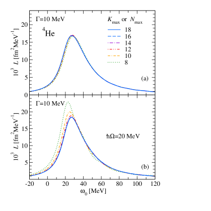
Figure 2: (Color online) Convergence of $L(\omega_{0},\Gamma)$ in ⁴He with $\Gamma=10$ MeV as a function of $K_{\rm max}$ in the EIHH expansion (a). Convergence of the LIT-CCSD equations with $\Gamma=10$ MeV as a function of $N_{\rm max}$ for an HO frequency of $\hbar\Omega=20$ MeV (b).

In Figure 2, the LIT of the ⁴He dipole response function is shown as a function of $\omega_{0}$ at fixed $\Gamma=10$ MeV. In panel (a) the EIHH results are presented for different model space sizes, represented by different values of the grandangular momentum $K_{\rm max}$. The convergence is fast and excellent. In panel (b) we show the results computed within the LIT-CCSD approach in model spaces of $N_{\rm max}=2n+l=8,10,12,\ldots 18$ and for a value of the underlying harmonic oscillator (HO) frequency of $\hbar\Omega=20$ MeV. Compared to the EIHH calculations, the LIT-CCSD approach shows a larger difference between the smallest and largest model space results. However, the LIT is well converged when $N_{\rm max}=18$ is used and does not change when varying the underlying HO frequency.

At this point it is interesting to compare both the EIHH and LIT-CCSD converged results. In Figure 3, we compare the LITs for the values of $\Gamma=20$ and 10 MeV in panel (a) and (b), respectively. The LIT-CCSD results are shown to overlap for two values of the harmonic oscillator frequency. They also agree very well with the EIHH result, especially for $\Gamma=20$ MeV. For the finer resolution scale of $\Gamma=10$ MeV, some slight differences are observed. It is known that calculations of the LIT with smaller $\Gamma$ tend to be more cumbersome. In fact as $\Gamma$ decreases the Lorentzian kernel approaches the $\delta-$function, facing again the continuum problem (for $\omega_{0}$ above the break-up threshold). Consequently the Lorentz state approaches the vanishing boundary condition at further and further distances. However, since the convergence of the LIT is very good, as also demonstrated by the $\hbar\Omega$-independence, we tend to attribute the small differences with respect to the EIHH result to the truncations inherent in the LIT-CCSD approximation.

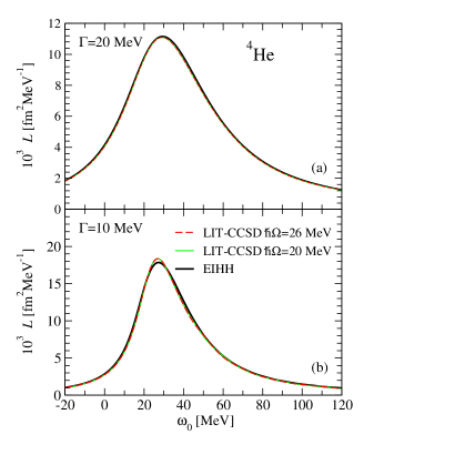
Figure 3: (Color online) Comparison of $L(\omega_{0},\Gamma)$ in ⁴He at $\Gamma=20$ (a), and $\Gamma=10$ (b), calculated in the LIT-CCSD scheme with $N_{\rm max}=18$ and two values of $\hbar\Omega=20$ and $26$ MeV against the LIT from EIHH.

To further quantify the role of the truncation, it is interesting to compare the dipole response functions obtained by the inversions of both the calculated LITs. For the inversions we use the method outlined in Refs. Efros et al. (1999); Andreasi, D. et al. (2005), which looks for the “regularized solution” of the integral transform equation. We regularize the solution by the following nonlinear ansatz

$$S(\omega)=\omega^{3/2}\exp\left(-\alpha\pi(Z-1)\sqrt{2\mu\over\omega}\right)\sum_{i}^{\nu}c_{i}e^{-\frac{\omega}{i\beta}}\,,$$ (47)

where $\beta$ is a nonlinear parameters. Since the first channel involves the Coulomb force between the emitted proton and the remaining nucleus with $(Z-1)$ protons a Gamow prefactor is included, $\alpha$ denotes the fine structure constant, and $\mu$ is the reduced mass of the proton and ${}^{15}N$ system. The coefficients $c_{i}$ and the parameter $\beta$ are obtained by a least square fit of the calculated LIT with the integral transform of the regularized ansatz in Eq. (47), requiring that the resulting response function is zero below the threshold energy $\omega_{\rm th}$, where particle emission starts. For the ⁴He case, where the first break-up channel is the proton-triton, $\omega_{\rm th}$ is obtained by the difference of the binding energies of ⁴He and ³H. The CCSD approximation and the particle-removed equation-of-motion method Gour et al. (2006); Hagen et al. (2010) lead to binding energies $23.97$ and $7.37$ MeV for ⁴He and ³H, respectively, leading to $\omega_{\rm th}=16.60$ MeV. With the N³LO two-body interaction precise binding energies are obtained from the EIHH method and are $25.39$ ($7.85$) MeV for ⁴He (³H), leading to a slightly different $\omega_{\rm th}=17.54$ MeV. Because for ⁴He we know the precise threshold results with the N³LO potential, we require the response function to be zero below 17.54 MeV, also when we invert the LIT-CCSD calculations.

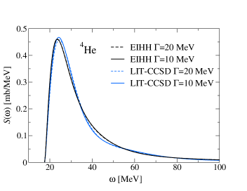
Figure 4: (Color online) Comparison of the ⁴He dipole response function calculated with LIT-CCSD ($\hbar\Omega=20$ MeV and $N_{\rm max}=18$) with the EIHH result. Inversions of the LITs with $\Gamma=10$ and 20 are performed.

Figure 4 shows the comparison of the response functions obtained by inverting the LIT from the LIT-CCSD and EIHH methods. For the LIT-CCSD calculations, we found that the inversions are insensitive to $\hbar\Omega$. In principle the inversion should also not depend on the parameter $\Gamma$. We employ $\Gamma=10$ MeV and $\Gamma=20$ MeV to gauge the quality of the inversions. For the EIHH, the inversions obtained from the LITs at $\Gamma=10$ and 20 MeV overlap very nicely, proving the precision of these calculations. In case of the LIT-CCSD, the two values of $\Gamma$ lead to slightly different inversion, as shown in Figure  4. Such a difference is small and can be viewed as a numerical uncertainty associated with the inversion. Overall, the LIT-CCSD response function is close to the virtually exact EIHH result. Apparently, the small deviations between the LIT-CCSD and the EIHH for the LIT in Figure 3 translates into small deviations in the response function for energies between about $\omega=30$ and $50$ MeV.

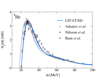
Figure 5: (Color online) Comparison of the ⁴He dipole cross section calculated with LIT-CCSD and experimental data from Arkatov et al. Arkatov et al. (1979), Nilsson et al. Nilsson et al. (2005) and Raut et al. Raut et al. (2012). The grey and blue bands differ simply by a shift of the theoretical threshold (grey) to the experimental one (dark/blue) (see text).

Finally, for completeness we present a comparison with experimental data on ⁴He. Extensive studies have been done in the past concerning the GDR in ⁴He, both from the theoretical and experimental point of view. Three-nucleon forces are typically included in the theory (see, e.g., Refs. Gazit et al. (2006a); Quaglioni and Navrátil (2007)), thus a comparison with data is not conclusive using two-body forces only. However, even a qualitative comparison is instructive, especially in the light of addressing heavier nuclei in the next sessions.

In Figure 5 we compare the photoabsorption cross section calculated in LIT-CCSD (the band width in the theoretical curves is obtained by filling the difference between the $\Gamma=10$ and 20 MeV inversions) with a selection of the available experimental data. The $E1$ photodisintegration cross section is related to the dipole response as

$$\sigma_{\gamma}^{E1}(\omega)=4\pi^{2}\alpha\omega S(\omega)\,,$$ (48)

with $\alpha$ being the fine structure constant. Arkatov et al. Arkatov et al. (1979) measured the photodisintegration cross section spanning a quite large energy range. More recent data by Nilsson et al. Nilsson et al. (2005) and Raut et al. Raut et al. (2012) cover a narrower range (see Ref. Bacca and Pastore (2014) for an update on all the measurements and calculations). In Figure 5, the grey curve represents the calculation where the theoretical threshold is used in the inversion. One notices that this is not as the experimental one, because the used Hamiltonian misses the contribution of the three-body force to the binding energies of ⁴He and³H. Thus, as typically done in the literature, to take this trivial binding effect into account we shift the theoretical (grey) curve to the experimental threshold (note that the consistent theoretical threshold is still used in the inversion procedure). It is evident that the theory describes the experimental data qualitatively, so it is interesting to address heavier nuclei.

V Application to ¹⁶O

The ⁴He benchmark suggests that the LIT-CCSD method can be employed for the computation of the dipole response, and that theoretical uncertainties with respect to the model space and the inversion of the LIT are well controlled. Thus, we turn our attention to a stable medium-mass nucleus, such as ¹⁶O.

First, we investigate the convergence of the LIT as a function of the model space size. In Figure 6, we present the LITs for $\Gamma=20$ MeV (panel (a)) and $\Gamma=10$ MeV (panel (b)) with $N_{\rm max}$ ranging from 8 up to 18. The convergence is rather good and it is better for the larger value of $\Gamma$. As indicated above, the smaller the width $\Gamma$, the more difficult is to converge in a LIT calculation. For $\Gamma=10$ a small difference of about about $2\%$ between $N_{\rm max}=16$ and $N_{\rm max}=18$ is found.

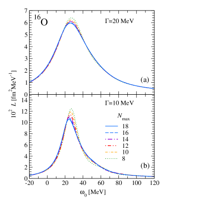
Figure 6: (Color online) Convergence of $L(\omega_{0},\Gamma)$ in ¹⁶O at $\Gamma=20$ MeV (a) and $\Gamma=10$ (b) for different values of $N_{\rm max}$ and an HO frequency of $\hbar\Omega=26$ MeV.

Before inverting the transform, it is first interesting to investigate the $\hbar\Omega$-dependence of our results and compare the theory with the integral transform of data. In Figure 7, LITs from our LIT-CCSD calculations with the largest model space size of $N_{\rm max}=18$ and two different HO frequencies of $\hbar\Omega=20$ and $26$ MeV are shown. As one can notice, there is a residual $\hbar\Omega$ dependence of roughly $4\%$, which is small and can be considered as the error bar of the numerical calculation. Overall, the theoretical error associated of our LIT for $\Gamma=10$ MeV in the LIT-CCSD scheme amounts to $5\%$.

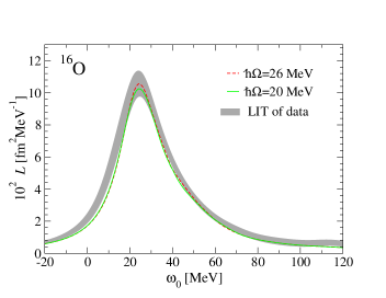
Figure 7: (Color online) Comparison of $L(\omega_{0},\Gamma)$ in ¹⁶O at $\Gamma=10$ calculated in the LIT-CCSD scheme with $N_{\rm max}=18$ and two values of $\hbar\Omega=20$ and $26$ MeV against the LIT of the experimental data from Ahrens et al. Ahrens et al. (1975).

The photodisintegration data measured by Ahrens et al. Ahrens et al. (1975) cover a broad energy range. Therefore it is possible to apply the LIT (Eq. (3)) on the response function extracted from the data by Eq. (48). This allows us to compare the experimental and theoretical results, as done in Figure 7 (the area between the grey lines represents the data error band). Our theoretical predictions agree with the experimental LIT within the uncertainties in almost all the $\omega_{0}$ range. Only from $\omega_{0}=0$ to about $15$ MeV, the theory slightly underestimates the data. Since the Lorentzian kernel in Eq. (3) is a representation of the $\delta$-function the integral in $\omega_{0}$ of $L(\omega_{0},\Gamma)$ is the same as the integral in $\omega$ of $S(\omega)$. Also peak positions are approximately conserved. Consequently, from Figure 7 we can infer that the LIT-CCSD calculation will reproduce the centroid of the experimental dipole response and the total strength.

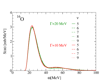
Figure 8: (Color online) The dipole response function of ¹⁶O obtained by inverting $L(\omega_{0},\Gamma)$ at $\Gamma=20$ and 10 MeV for different values $\nu$ of the basis functions in Eq. (47).

At this point, we perform the inversion of the computed LIT using the ansatz of Eq. (47), in order to compare with the cross section directly. Let us first investigate the stability of the inversions. In Figure 8 we show the inversions of the ¹⁶O LITs at $\Gamma=20$ and 10 MeV for different values $\nu$ of the basis functions in Eq. (47). Within the CCSD scheme, the binding energy of ¹⁶O is 107.24 MeV and with the more precise perturbative-triples approach, $\Lambda$-CCSD(T) Taube and Bartlett (2008); Hagen et al. (2010), it becomes 121.47 MeV. The threshold energy, in this case is the difference between the binding energy of ¹⁶O and ¹⁵N, and is computed using the particle-removed equation-of-motion theory. For the ¹⁶O photodisintegration reaction $\omega_{\rm th}$ becomes then $14.25$ MeV and in the inversion we require the response function to be zero below this threshold. For a fixed value of $\Gamma$, several choices of the number of basis states (from $\nu=5$ to 9) lead to basically the same inversion. For ¹⁶O the inversions obtained from the LIT at $\Gamma=10$ MeV are slightly different than those obtained from the LIT at $\Gamma=20$ MeV. This is due to the fact that the corresponding LITs themselves are converged only at a few-percent level and not to the sub-percent level. Because such a difference is very small, we will interpret it as a numerical error of the inversion and consider a band made by all of these inversions together as our final result in the LIT-CCSD scheme. The latter is presented in Figure 9 in comparison to the data by Ahrens et al. Ahrens et al. (1975) and also to the more recent evaluation by Ishkhanov et al. Ishkhanov et al. (2002); Ishkhanov and Orlin (2004). The grey curve represents the LIT-CCSD result plotted starting from the theoretical threshold and the dark/blue curve is plotted from the experimental threshold, in analogy to what is done in Fig. 5. The position of the GDR in ¹⁶O is rather well reproduced by our calculations. We find that the theoretical width of the GDR is larger than the experimental one, while the tail region between 40 and 100 MeV is well described within uncertainties.

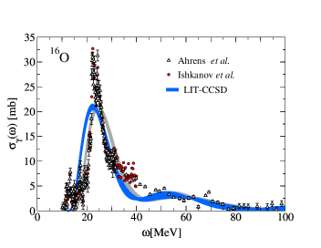
Figure 9: (Color online) Comparison of the ¹⁶O dipole cross section calculated in the LIT-CCSD scheme against experimental data by Ahrens et al. Ahrens et al. (1975) (triangles with error bars), and Ishkhanov et al. Ishkhanov et al. (2002) (red circles). The grey curve starts from the theoretical threshold, while the dark/blue curve is shifted to the experimental threshold.

In literature, the Thomas-Reiche-Kuhn sum rule is often discussed in relation to the the photoabsorption cross sections. It is obtained by the following integral

$$\int_{\omega_{\rm th}}^{\infty}d\omega\sigma(\omega)=59.74(NZ/A){\rm~{}MeVmb~{}}(1+\kappa)\,$$ (49)

and $\kappa$ is the so-called enhancement factor. The latter is related to the contribution of exchange terms in the nucleon-nucleon force and their induced correlations Orlandini and Traini (1991)). When integrating the theoretical photoabsorption cross section up to $100$ MeV we obtain an enhancement $\kappa=0.57-0.58$ of the Thomas-Reiche-Kuhn sum rule $\left[59.74\frac{NZ}{A}{\rm MeV~{}mb}(1+\kappa)\right]$.

VI Application to ²²O

It is interesting to apply the present method to the study of the dipole response function of the neutron-rich nucleus ²²O.

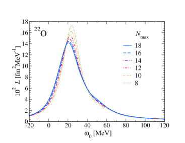
Figure 10: (Color online) Convergence of $L(\omega_{0},\Gamma)$ in ²²O at $\Gamma=10$ MeV as a function of $N_{\rm max}$ for an harmonic oscillator frequency of $\hbar\Omega=24$ MeV.

Figure 10 shows the convergence of the LIT, as a function of the model space size, presenting $L(\omega_{0},\Gamma)$ for $\Gamma=10$ MeV with $N_{\rm max}$ ranging from 8 up to 18. We observe that the convergence rate is comparable to that found in ¹⁶O.

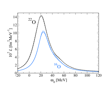
Figure 11: (Color online) Comparison of $L(\omega_{0},\Gamma)$ at $\Gamma=10$ MeV for ²²O and ¹⁶O. Different harmonic oscillator frequencies have been used: $\hbar\Omega$ = 20 and 24 MeV for ¹⁶O (dashed and full blue lines) and $\hbar\Omega$ = 24 and 26 MeV for ²²O (dashed and full black lines).

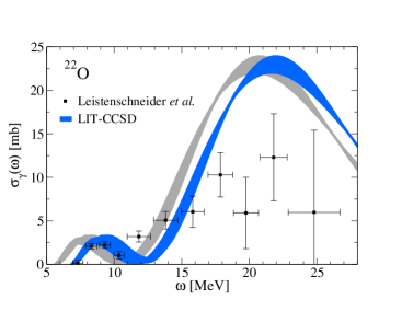
Figure 12: (Color online) Comparison of the LIT-CCSD dipole cross section of ²²O with the photoneutron data of Ref. Leistenschneider et al. (2001). The grey curve starts from the theoretical threshold, while the dark/blue curve is shifted to the experimental threshold.

In Fig. 11 we compare the LIT for ²²O versus ¹⁶O for the width $\Gamma=10$ MeV. One notices that the ²²O total strength is larger than that of ¹⁶O. The total dipole strength is the bremsstrahlung sum rule (BSR)

$${\rm BSR}\equiv\int_{\omega_{\rm th}}^{\infty}d\omega S(\omega)=\langle 0|{\hat{D_{0}}}^{\dagger}\hat{D_{0}}|0\rangle\,.$$ (50)

Using the definition of the LIT, Eq. (3), and the properties of the Lorentzian kernel the BSR can also be written as

$${\rm BSR}=\int_{-\infty}^{\infty}d\omega_{0}L(\omega_{0},\Gamma)\;.$$ (51)

In both ways we obtain a value of 4.6 and 6.7 fm² for ¹⁶O and ²²O, respectively.

We note that the BSR can also be written as Brink (1957)

$${\rm BSR}\propto\left(\frac{NZ}{A}\right)^{2}{R}_{PN}^{2}\ .$$ (52)

Here ${R}_{PN}$ is the difference between the proton and the neutron centers of mass. If one assumes that the two centers of mass do not differ much in ¹⁶O and ²²O, difference in the BSR between ¹⁶O and ²² O is explained by the different neutron numbers and mass numbers. This is indeed what we observe within 10%.

Inverting the LIT and imposing the strength to be zero below the N³LO threshold energy of 5.6 MeV, we find the cross section displayed in Fig. 12. In this case we did not include the Gamow prefactor of Eq. (47) in the inversion, because the first channel corresponds to the emission of a neutron. One notices the appearance of a small peak at low energy. The existence of such a peak is a stable feature, independent on the inversion uncertainties. The latter are represented by the band width of the curves, obtained by inverting LITs with $\Gamma=5,10$ and 20 MeV and varying the $\nu$ in Eq. (47). As before, the grey curve corresponds to the LIT-CCSD result starting from the theoretical threshold, while the dark/blue curve is shifted to the experimental threshold. After this shift is performed, it is even more evident that the strength of this low-lying peak reproduces the experimental one. Such low-energy peaks in the dipole response are debated as dipole modes of the excess neutrons against an ¹⁶O core, see, also Ref. Repko et al. (2013). However, like for the experimental result, the strength of this low energy peak only exhausts about 10% of the cluster sum rule Alhassid et al. (1982) inspired by that interpretation.

This is not the first time that the LIT approach suggests the existence of a low-energy dipole mode. In fact Ref. Bacca et al. (2002) predicts a similar, but much more pronounced peak in ⁶He for semirealistic interactions. In that case, however, due to the much bigger ratio of the neutron halo to the core, the cluster sum rule is fully exhausted.

When integrating the theoretical photo-absorption cross section up to $100$ MeV we obtain an enhancement $\kappa=0.54-0.57$ of the Thomas-Reiche-Kuhn sum rule.

VII Application to ⁴⁰Ca

The computational cost of the CC method scales mildly with respect to the mass number $A$ and the size of the model space. This allows us to tackle the GDR in ⁴⁰Ca, for which data by Ahrens et al. Ahrens et al. (1975) exist from photoabsorption on natural samples of calcium.

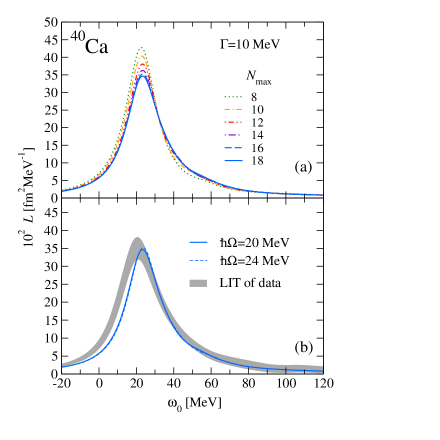
Figure 13: (Color online) Convergence of $L(\omega_{0},\Gamma)$ in ⁴⁰Ca at $\Gamma=10$ MeV as a function of $N_{\rm max}$ for an harmonic oscillator frequency of $\hbar\Omega=20$ MeV (a). Comparison of $L(\omega_{0},\Gamma)$ in ⁴⁰Ca at $\Gamma=10$ calculated in the LIT-CCSD scheme with $N_{\rm max}=18$ and two values of $\hbar\Omega=20$ and $24$ MeV against the LIT of the experimental data from Ahrens et al. Ahrens et al. (1975) (b).

In Fig. 13(a) we show the convergence of the LIT calculations as a function of $N_{\rm max}$ for a fixed value of the HO frequency $\hbar\Omega=20$ MeV and for $\Gamma=10$ MeV. It is apparent that the convergence is of the same quality as for the oxygen isotopes. In the bottom panel, a comparison of two LITs with different underlying HO parameter ($\hbar\Omega=20$ and 24 MeV) is presented, indicating that the residual $\hbar\Omega$-dependence is small. A comparison with the LIT of the experimental data by Ahrens et al. is also shown, where the error is represented by the bands. For ⁴⁰Ca the location of the GDR predicted using the N³LO nucleon-nucleon interaction is found at slightly larger excitation energy with respect to the experiment. This feature is also reflected when the LIT is inverted and the photoabsorption cross section is calculated in the dipole approximation, using Eq. (48). In this calculation we apply the ansatz of Eq. (47) using the threshold energy $\omega_{\rm th}=12.8$ MeV obtained with the particle-removed equation-of-motion method Gour et al. (2006); Hagen et al. (2010). By taking different widths of the LIT to invert ($\Gamma=5,10$ and 20 MeV) and by varying the number $\nu$ in Eq. (47), we obtain the grey band in Fig. 14. In comparison to the cross section data by Ahrens et al. Ahrens et al. (1975), the theoretical prediction of the GDR is quite encouraging. A giant resonance is clearly seen. However, it is slightly broader, lower in strength and situated at higher energy than the experimental GDR. Because the threshold energy with the N³LO nucleon-nucleon interaction is quite different than the experimental threshold, located at about 8.3 MeV, in Fig. 14, we also show (in dark blue) the theoretical curves shifted on the experimental threshold energy.

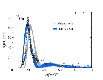
Figure 14: (Color online) Comparison of the LIT-CCSD dipole cross section of ⁴⁰Ca with the photoabsorption data of Ref. Ahrens et al. (1975). The grey curve starts from the theoretical threshold, while the dark/blue curve is shifted to the experimental threshold.

When integrating the theoretical photo-absorption cross section up to $100$ MeV we obtain an enhancement $\kappa=0.69-0.73$ of the Thomas-Reiche-Kuhn sum rule.

Let us also consider the dipole polarizability because of its considerable experimental and theoretical interest Tamii et al. (2011); Piekarewicz et al. (2012). From the dipole response function $S(\omega)$ one can obtain the electric dipole polarizability

$$\alpha_{E}=2\alpha\int_{\omega_{\rm th}}^{\infty}d\omega\frac{S(\omega)}{\omega}$$ (53)

as an inverse energy weighted sum rule. In analogy to Ref. Gazit et al. (2006b), electric dipole polarizability can be also obtained directly from the Lanczos approach  Goerke et al. (2012); Miorelli et al. (2014); Nevo Dinur et al. (2014), avoiding the inversion of the integral transform. The removal of center of mass spuriosities for this observable can be done in the same way as explained in Section III.3. In this case

$$\alpha_{E}=2\alpha\sum_{\nu}\frac{|\langle\varphi_{\nu}^{N}|\Theta|0\rangle|^{2}}{\epsilon_{\nu}^{N}}$$ (54)

and the spurious states can be removed from the sum. Both from the Lanczos approach and integrating the response function up to 100 MeV we obtain $\alpha_{E}=1.47$ fm³ within $5\%$. With the present N³LO nucleon-nucleon interaction we predict a polarizability for ⁴⁰Ca, which is rather low in comparison to the experimental value of $\alpha^{\rm exp}_{E}=2.23(3)$ fm³ Ahrens et al. (1975). If we integrate the strength after shifting it to the experimental threshold (dark/blue curve in Fig. 14) we obtain roughly $\alpha_{E}=1.82$ fm³, thus moving in the direction of the experimental value. We also note that if we integrate the cross section data by Ahrens et al. Ahrens et al. (1975) we obtain $1.95(26)$ fm³ for the dipole polarizability. It is worth to mention that with the present nucleon-nucleon interaction ⁴⁰Ca is about $20$ MeV overbound and with a charge radius $R_{\rm ch}=3.05$ fm, which is considerably smaller than the experimental value of $3.4776(19)$ fm Angeli and Marinova (2013). This points towards a general problem of the present Hamiltonian, which does not provide good saturation properties of nuclei, leading to too small radii and consequently too small polarizabilities.

VIII Conclusions

We presented in detail an approach that combines the Lorentz integral transform with the coupled-cluster method, named LIT-CC, for the computation of the dipole response function in ⁴He, ^16,22O and ⁴⁰Ca. The benchmark of this method against the EIHH in ⁴He gives us the necessary confidence for the computation in heavier nuclei. The LIT-CCSD approximation yielded results for the total photonuclear dipole cross section of oxygen and calcium isotopes that are in semi-quantitative agreement with data. This opens the way for interesting investigations of the response functions of heavier nuclei, also beyond the stability valley.

The comparison of the LITs of the response functions of ¹⁶O and ²²O shows a larger total area of the latter (corresponding to the relative bremsstrahlung sum rule) and a slight shift of the peak to lower energy. Such a shift already envisages the possibility of more strength in that region. This becomes manifest after the inversion. For ²²O we found a very interesting dipole cross section exhibiting two peaks: A small one at 8-9 MeV and a larger one at 21-22 MeV. We also extend our calculations further out in mass number, presenting first results on the GDR of ⁴⁰Ca. In this case we observe that, with respect to experiment, the N³LO nucleon-nucleon interaction leads to larger excitation energy of the GDR, which is consistent with the over-binding, the too small charge radius and dipole polarizability we obtain for ⁴⁰Ca. The results presented here also open the way to systematic investigations of more general electro-weak responses of medium-mass nuclei with an ab-initio approach.