Asymptotic goodness-of-fit tests for the Palm mark distribution of stationary point processes with correlated marks

Abstract

We consider spatially homogeneous marked point patterns in an unboundedly expanding convex sampling window. Our main objective is to identify the distribution of the typical mark by constructing an asymptotic $\chi^{2}$-goodness-of-fit test. The corresponding test statistic is based on a natural empirical version of the Palm mark distribution and a smoothed covariance estimator which turns out to be mean square consistent. Our approach does not require independent marks and allows dependences between the mark field and the point pattern. Instead we impose a suitable $\beta$-mixing condition on the underlying stationary marked point process which can be checked for a number of Poisson-based models and, in particular, in the case of geostatistical marking. In order to study test performance, our test approach is applied to detect anisotropy of specific Boolean models.

, and

1 Introduction

Marked point processes (MPPs) are versatile models for the statistical analysis of data recorded at irregularly scattered locations. The simplest marking scenario is independent marking, where marks are given by a sequence of independent and identically distributed random elements, which is also independent of the underlying point pattern of locations. A more complex class of models considers a so-called geostatistical marking, where the marks are determined by the values of a random field at the given locations. Although the random field usually exhibits intrinsic spatial correlations, it is assumed to be independent of the location point process (PP). However, in many real datasets interactions between locations and marks occur. Moreover, many marked point patterns arising in models from stochastic geometry such as edge centers in (anisotropic) Voronoi-tessellations marked by orientation or PPs marked by nearest-neighbour distances do not fit the setting of geostatistical marking. For recent asymptotic approaches to mark correlation analysis based on mark variogram and mark covariance functions, we refer to [7, 8, 10]. The main goal of this paper is to investigate estimators of the Palm mark distribution $P_{M}^{\mathbf{o}}$ in point patterns exhibiting correlations between different marks as well as between marks and locations. The probability measure $P_{M}^{\mathbf{o}}$ can be interpreted as the distribution of the typical mark which denotes the mark of a randomly chosen point of the pattern. For any mark set $C$, we consider the scaled deviations $Z_{k}(C)=\sqrt{|W_{k}|}((\widehat{P}{}^{\mathbf{o}}_{M})_{k}(C)-P_{M}^{\mathbf{o}}(C))$ as measure of the distance between $P_{M}^{\mathbf{o}}$ and an empirical Palm mark distribution $(\widehat{P}{}^{\mathbf{o}}_{M})_{k}$. In [12], we prove asymptotic normality of the scaled deviation vector $\mathbf{Z}_{k}=(Z_{k}(C_{1}),\ldots,Z_{k}(C_{\ell}))^{T}$ under appropriate strong mixing conditions when the observation window $W_{k}$ with volume $|W_{k}|$ grows unboundedly in all directions as $k\to\infty$. In this study, we in particular discuss consistent estimators for the covariance matrix of the Gaussian limit of $\mathbf{Z}_{k}$. This enables us to construct asymptotic $\chi^{2}$-goodness-of-fit tests for the Palm mark distribution $P_{M}^{\mathbf{o}}$. In a simulation study we apply our testing methodology to the directional analysis of random surfaces. For this purpose, we consider Cox processes on the boundary of Boolean models, mark them with the local outer normal direction and test for a hypothetical directional distribution. This allows to identify the rose of directions of the surface process associated with the Boolean model and represents an alternative to a Monte Carlo test for the rose of direction suggested in [1]. The occurring MPPs differ fundamentally from the setting of independent and geostatistical marking, for which functional central limit theorems (CLTs) and corresponding tests have been derived in [14, 19]. In general, they also do not represent $m$-dependent MPPs.

Our paper is organized as follows. Section 2 introduces basic notation and definitions. In Section 3, we present our main results, which are proved in Section 4. In Section 5, we briefly discuss some models satisfying the assumptions needed to prove our asymptotic results. In the final Section 6, we study the performance of the proposed tests by simulations.

2 Stationary marked point processes

An MPP $\mathbf{X}_{M}=\sum_{n\geq 1}\delta_{(X_{n},M_{n})}$ is a random locally finite counting measure (see [4], Volume II, Chapter 9.1) on the Borel sets of ${\mathbb{R}}^{d}\times\mathbb{M}$ with atoms $(X_{n},M_{n})$, where the mark space $\mathbb{M}$ is Polish endowed with its Borel $\sigma$-algebra $\mathcal{B}(\mathbb{M})$. Formally, $\mathbf{X}_{M}$ is a random element with values in the space $\mathsf{N}_{\mathbb{M}}$ of locally finite counting measures $\varphi(\cdot)$ on ${\mathcal{B}}({\mathbb{R}}^{d}\times{\mathbb{M}})$, where $\mathsf{N}_{\mathbb{M}}$ is equipped with the $\sigma$-algebra generated by all sets of the form $\{\varphi\in{\mathsf{N}}_{{\mathbb{M}}}\colon\ \varphi(B\times C)=j\}$ for $j\geq 0$, bounded $B\in\mathcal{B}({\mathbb{R}}^{d})$, and $C\in{\mathcal{B}}({\mathbb{M}})$. Throughout we assume that $\mathbf{X}_{M}$ is simple, that is, all locations $X_{n}$ in ${\mathbb{R}}^{d}$ have multiplicity $1$ regardless which mark they have. In what follows, we only consider stationary MPPs, which means that

$$\mathbf{X}_{M}\stackrel{{\scriptstyle\mathrm{D}}}{{=}}\sum_{n\geq 1}\delta_{(X_{n}-x,M_{n})}\qquad\mbox{for all }x\in{\mathbb{R}}^{d}.$$

We always assume that the intensity $\lambda={\mathbb{E}}\mathbf{X}_{M}([0,1)^{d}\times\mathbb{M})$ is finite.

2.1 Palm mark distribution

For a stationary MPP $\mathbf{X}_{M}$ the probability measure $P_{M}^{\mathbf{o}}$ on $\mathcal{B}(\mathbb{M})$ defined by

$$P_{M}^{\mathbf{o}}(C)=\frac{1}{\lambda}\mathbb{E}\mathbf{X}_{M}\bigl{(}[0,1)^{d}\times C\bigr{)},\qquad C\in\mathcal{B}(\mathbb{M}),$$ (1)

is called the Palm mark distribution of $\mathbf{X}_{M}$. It can be interpreted as the conditional distribution of the mark of an atom of $\mathbf{X}_{M}$ located at the origin $\mathbf{o}$. A random element $M_{0}$ in $\mathbb{M}$ with distribution $P_{M}^{\mathbf{o}}$ is called typical mark of $\mathbf{X}_{M}$.

Definition 2.1.

An increasing sequence $\{W_{k}\}$ of convex and compact sets in ${\mathbb{R}}^{d}$ such that $\varrho(W_{k})=\sup\{r>0\colon\ B(x,r)\subset W_{k}$ for some $x\in W_{k}\}\rightarrow\infty$ as $k\to\infty$ is called a convex averaging sequence (briefly CAS). Here $B(x,r)$ denotes the closed ball (w.r.t. the Euclidean norm $\|\cdot\|$) with midpoint at $x\in{\mathbb{R}}^{d}$ and radius $r\geq 0$.

In the following, $|\cdot|$ denotes $d$-dimensional Lebesgue measure and ${\cal H}_{d-1}$ is the surface content (i.e., $(d-1)$-dimensional Hausdorff measure). Some results from convex geometry applied to CAS $\{W_{k}\}$ yield the following inequalities (see [2] and [14])

$$\frac{1}{\varrho(W_{k})}\leq\frac{{\cal H}_{d-1}(\partial W_{k})}{|W_{k}|}\leq\frac{d}{\varrho(W_{k})}\quad\mbox{and}\quad 1-\frac{|W_{k}\cap(W_{k}-x)|}{|W_{k}|}\leq\frac{d\|x\|}{\varrho(W_{k})}$$ (2)

for $\|x\|\leq\varrho(W_{k})$. Moreover, using the notation ${\overline{H}}_{k}=\{z\in\mathbb{Z}^{d}\colon\ |E_{z}\cap W_{k}|>0\}$, where $E_{z}=[-1/2,1/2)^{d}+z$ for $z\in\mathbb{Z}^{d}$, we have shown in [11, 12] that for a CAS $\{W_{k}\}$

$$1\leq\frac{\#{\overline{H}}_{k}}{|W_{k}|}\leq 1+\frac{|W_{k}\oplus B(o,\sqrt{d})|-|W_{k}|}{|W_{k}|}\mathop{\longrightarrow}_{k\to\infty}1,$$ (3)

which follows from Steiner’s formula (see [20], page 197), and (2). If $\mathbf{X}_{M}$ is ergodic (for a precise definition see [4], Volume II, page 194), the individual ergodic theorem applied to MPPs (see Theorem 12.2.IV and Corollary 12.2.V in [4], Volume II) provides the $\mathbb{P}\mbox{-}\mathrm{a.s.}$ limits

$$\widehat{\lambda}_{k}=\frac{\mathbf{X}_{M}(W_{k}\times{\mathbb{M}})}{|W_{k}|}\,\displaystyle\mathop{\longrightarrow}^{\mathbb{P}\mbox{-}\mathrm{a.s.}}_{k\to\infty}\,\lambda\quad\mbox{and}\quad\bigl{(}\widehat{P}{}^{\mathbf{o}}_{M}\bigr{)}_{k}(C)=\frac{\mathbf{X}_{M}(W_{k}\times C)}{\mathbf{X}_{M}(W_{k}\times{\mathbb{M}})}\,\displaystyle\mathop{\longrightarrow}^{\mathbb{P}\mbox{-}\mathrm{a.s.}}_{k\to\infty}\,P^{\mathbf{o}}_{M}(C)$$ (4)

for any $C\in\mathcal{B}(\mathbb{M})$ and an arbitrary CAS $\{W_{k}\}$.

2.2 Factorial moment measures and the covariance measure

For any integer $m\geq 1$, the $m$th factorial moment measure $\alpha_{\mathbf{X}_{M}}^{(m)}$ of the MPP $\mathbf{X}_{M}$ is defined on $\mathcal{B}(({\mathbb{R}}^{d}\times{\mathbb{M}})^{m})$ by

$$\alpha_{\mathbf{X}_{M}}^{(m)}\Biggl{(}\mathop{\mbox{{$\!\times$}}}_{i=1}^{m}(B_{i}\times C_{i})\Biggr{)}={\mathbb{E}}{\sum^{\neq}_{n_{1},\ldots,n_{m}\geq 1}}\prod_{i=1}^{m}\bigl{(}\mathbh 1_{B_{i}}(X_{n_{i}})\mathbh 1_{C_{i}}(M_{n_{i}})\bigr{)},$$ (5)

where the sum $\sum_{n_{1},\ldots,n_{m}\geq 1}^{\neq}$ runs over all $m$-tuples of pairwise distinct indices $n_{1},\ldots,n_{m}\geq 1$ for bounded $B_{i}\in\mathcal{B}({\mathbb{R}}^{d})$ and $C_{i}\in\mathcal{B}(\mathbb{M}),i=1,\ldots,m$. We also need the $m$th factorial moment measure $\alpha_{\mathbf{X}}^{(m)}$ of the unmarked PP $\mathbf{X}(\cdot)=\mathbf{X}_{M}((\cdot)\times\mathbb{M})=\sum_{n\geq 1}\delta_{X_{n}}(\cdot)$ defined on $\mathcal{B}(({\mathbb{R}}^{d})^{m})$ by

$$\alpha_{\mathbf{X}}^{(m)}\Biggl{(}\mathop{\mbox{{$\!\times$}}}_{i=1}^{m}B_{i}\Biggr{)}=\alpha_{\mathbf{X}_{M}}^{(m)}\Biggl{(}\mathop{\mbox{{$\!\times$}}}_{i=1}^{m}(B_{i}\times\mathbb{M})\Biggr{)}\qquad\mbox{for bounded }B_{1},\ldots,B_{m}\in\mathcal{B}\bigl{(}{\mathbb{R}}^{d}\bigr{)}.$$

The stationarity of $\mathbf{X}_{M}$ implies that $\alpha_{\mathbf{X}}^{(m)}$ is invariant under diagonal shifts, which allows to define the $m$th reduced factorial moment measure $\alpha_{\mathbf{X},\mathrm{red}}^{(m)}$ uniquely determined by the following disintegration formula

$$\alpha_{\mathbf{X}}^{(m)}\Biggl{(}\mathop{\mbox{{$\!\times$}}}_{i=1}^{m}B_{i}\Biggr{)}=\lambda\int_{B_{1}}\alpha_{\mathbf{X},\mathrm{red}}^{(m)}\Biggl{(}\mathop{\mbox{{$\!\times$}}}_{i=2}^{m}(B_{i}-x)\Biggr{)}\,\mathrm{d}x\qquad\mbox{see \cite[cite]{[\@@bibref{}{Daley0307}{}{}]}, Volume II, Chapter 12.1}.$$ (6)

The weak correlatedness between parts of $\mathbf{X}$ over distant Borel sets may be expressed by the (factorial) covariance measure $\gamma_{\mathbf{X}}^{(2)}$ on $\mathcal{B}(({\mathbb{R}}^{d})^{2})$ defined by

$$\gamma_{\mathbf{X}}^{(2)}(B_{1}\times B_{2})=\alpha_{\mathbf{X}}^{(2)}(B_{1}\times B_{2})-\lambda^{2}|B_{1}||B_{2}|.$$

The reduced covariance measure $\gamma^{(2)}_{\mathbf{X},\mathrm{red}}\mathchoice{\nobreak\,\colon}{\nobreak\,\colon}{\nobreak\,\colon\;}{\nobreak\,\colon\;}\mathcal{B}({\mathbb{R}}^{d})\to[-\infty,\infty]$ is in general a signed measure defined in analogy to (6) with $\gamma_{\mathbf{X}}^{(2)}$ instead of $\alpha_{\mathbf{X}}^{(2)}$, which shows that

$$\gamma^{(2)}_{\mathbf{X},\mathrm{red}}(B)=\alpha^{(2)}_{\mathbf{X},\mathrm{red}}(B)-\lambda|B|\qquad\mbox{for bounded }B\in\mathcal{B}\bigl{(}{\mathbb{R}}^{d}\bigr{)}.$$

2.3 $m$-point Palm mark distribution

For fixed mark sets $C_{1},\ldots,C_{m}\in\mathcal{B}(\mathbb{M}),m\geq 1$, the $m$th factorial moment measure $\alpha_{\mathbf{X}_{M}}^{(m)}$ of the MPP (see (5)) can be regarded as a measure on $\mathcal{B}(({\mathbb{R}}^{d})^{m})$, which is absolutely continuous w.r.t. $\alpha_{\mathbf{X}}^{(m)}$. Thus, there exists a Radon–Nikodym density $P_{M}^{x_{1},\ldots,x_{m}}(C_{1}\times\cdots\times C_{m})$, such that for any $B_{1},\ldots,B_{m}\in\mathcal{B}({\mathbb{R}}^{d})$,

$$\alpha_{\mathbf{X}_{M}}^{(m)}\Biggl{(}\mathop{\mbox{{$\!\times$}}}_{i=1}^{m}(B_{i}\times C_{i})\Biggr{)}=\int_{\mathop{\times}_{i=1}^{m}B_{i}}P_{M}^{x_{1},\ldots,x_{m}}\Biggl{(}\mathop{\mbox{{$\!\times$}}}_{i=1}^{m}C_{i}\Biggr{)}\alpha_{\mathbf{X}}^{(m)}\bigl{(}\mathrm{d}(x_{1},\ldots,x_{m})\bigr{)}.$$ (7)

Since the mark space $\mathbb{M}$ is Polish, this Radon–Nikodym density can be extended to a regular conditional distribution of the mark vector $(M_{1},\ldots,M_{m})$ given that the corresponding atoms $X_{1},\ldots,X_{m}$ are located at pairwise distinct points $x_{1},\ldots,x_{m}$, that is,

$$P_{M}^{x_{1},\ldots,x_{m}}(C)=\mathbb{P}\bigl{(}(M_{1},\ldots,M_{m})\in C\mid X_{1}=x_{1},\ldots,X_{m}=x_{m}\bigr{)}\qquad\mbox{for }C\in\mathcal{B}\bigl{(}\mathbb{M}^{m}\bigr{)}.$$

For details we refer to [16], page 164. The above conditional distribution is called the $m$-point Palm mark distribution of $\mathbf{X}_{M}$. In case of a stationary simple MPP $\mathbf{X}_{M}$, it is easily checked that the one-point Palm mark distribution coincides with the Palm mark distribution defined in (1).

The next result is indispensable to study asymptotic properties of variance estimators for the empirical mark distribution. It extends a formula stated in [15] for unmarked PPs to the case of marked PPs. The proof of this extension relies essentially on (7). Details are left to the reader.

Lemma 2.1

Let $\mathbf{X}_{M}=\sum_{n\geq 1}\delta_{(X_{n},M_{n})}$ be an MPP satisfying ${\mathbb{E}}\mathbf{X}_{M}(B\times{\mathbb{M}})^{4}<\infty$ for all bounded $B\in\mathcal{B}({\mathbb{R}}^{d})$, and let $f\mathchoice{\nobreak\,\colon}{\nobreak\,\colon}{\nobreak\,\colon\;}{\nobreak\,\colon\;}{\mathbb{R}}^{d}\times{\mathbb{R}}^{d}\times\mathbb{M}^{2}\mapsto{\mathbb{R}}^{1}$ be a Borel-measurable function such that the second moment of $\sum_{p,q\geq 1}^{\neq}|f(X_{p},X_{q},M_{p},M_{q})|$ exists. Then,

$$\operatorname{Var}\Biggl{(}\sum^{\neq}_{p,q\geq 1}f(X_{p},X_{q},M_{p},M_{q})\Biggr{)}$$

$$\quad=\int_{({\mathbb{R}}^{d})^{2}}\int_{{{\mathbb{M}}}^{2}}f(x_{1},x_{2},u_{1},u_{2})\bigl{[}f(x_{1},x_{2},u_{1},u_{2})+f(x_{2},x_{1},u_{2},u_{1})\bigr{]}$$

$$\qquad\hskip 41.0pt{}\times P_{M}^{x_{1},x_{2}}\bigl{(}\mathrm{d}(u_{1},u_{2})\bigr{)}\alpha_{\mathbf{X}}^{(2)}\bigl{(}\mathrm{d}(x_{1},x_{2})\bigr{)}$$

$$\qquad{}+\int_{({\mathbb{R}}^{d})^{3}}\int_{{{\mathbb{M}}}^{3}}f(x_{1},x_{2},u_{1},u_{2})\bigl{[}f(x_{1},x_{3},u_{1},u_{3})+f(x_{3},x_{1},u_{3},u_{1})$$

$$\hskip 125.1pt\qquad{}+f(x_{2},x_{3},u_{2},u_{3})+f(x_{3},x_{2},u_{3},u_{2})\bigr{]}$$

$$\qquad\hskip 53.5pt{}\times P_{M}^{x_{1},x_{2},x_{3}}\bigl{(}\mathrm{d}(u_{1},u_{2},u_{3})\bigr{)}\alpha_{\mathbf{X}}^{(3)}\bigl{(}\mathrm{d}(x_{1},x_{2},x_{3})\bigr{)}$$

$$\qquad{}+\int_{({\mathbb{R}}^{d})^{4}}\int_{{{\mathbb{M}}}^{4}}f(x_{1},x_{2},u_{1},u_{2})f(x_{3},x_{4},u_{3},u_{4})$$

$$\qquad\hskip 54.0pt{}\times\bigl{[}P_{M}^{x_{1},x_{2},x_{3},x_{4}}\bigl{(}\mathrm{d}(u_{1},u_{2},u_{3},u_{4})\bigr{)}\alpha_{\mathbf{X}}^{(4)}\bigl{(}\mathrm{d}(x_{1},x_{2},x_{3},x_{4})\bigr{)}$$

$$\hskip 69.0pt\qquad{}-P_{M}^{x_{1},x_{2}}\bigl{(}\mathrm{d}(u_{1},u_{2})\bigr{)}P_{M}^{x_{3},x_{4}}\bigl{(}\mathrm{d}(u_{3},u_{4})\bigr{)}\alpha_{\mathbf{X}}^{(2)}\bigl{(}\mathrm{d}(x_{1},x_{2})\bigr{)}\alpha_{\mathbf{X}}^{(2)}\bigl{(}\mathrm{d}(x_{3},x_{4})\bigr{)}\bigr{]}.$$

2.4 $\beta$-mixing coefficient and covariance inequality

For any $B\in\mathcal{B}({\mathbb{R}}^{d})$, let ${\mathcal{A}}_{\mathbf{X}_{M}}(B)$ denote the sub-$\sigma$-algebra of ${\mathcal{A}}$ generated by the restriction of the MPP $\mathbf{X}_{M}$ to the set $B\times{\mathbb{M}}$. For any $B,B^{\prime}\in\mathcal{B}({\mathbb{R}}^{d})$, a natural measure of dependence between ${\mathcal{A}}_{\mathbf{X}_{M}}(B)$ and ${\mathcal{A}}_{\mathbf{X}_{M}}(B^{\prime})$ can be formulated in terms of the $\beta$-mixing (or absolute regularity, respectively, weak Bernoulli) coefficient

$$\beta\bigl{(}{\mathcal{A}}_{\mathbf{X}_{M}}(B),{\mathcal{A}}_{\mathbf{X}_{M}}\bigl{(}B^{\prime}\bigr{)}\bigr{)}=\frac{1}{2}\sup_{\{A_{i}\},\{A^{\prime}_{j}\}}\sum_{i,j}\bigl{|}\mathbb{P}\bigl{(}A_{i}\cap A_{j}^{\prime}\bigr{)}-\mathbb{P}(A_{i})\mathbb{P}\bigl{(}A_{j}^{\prime}\bigr{)}\bigr{|},$$ (9)

where the supremum is taken over all finite partitions $\{A_{i}\}$ and $\{A_{j}^{\prime}\}$ of $\Omega$ such that $A_{i}\in{\mathcal{A}}_{\mathbf{X}_{M}}(B)$ and $A_{j}^{\prime}\in{\mathcal{A}}_{\mathbf{X}_{M}}(B^{\prime})$ for all $i,j$, see [5] or [3] for a detailed discussion of this and other mixing coefficients. To quantify the degree of dependence of the MPP $\mathbf{X}_{M}$ on disjoint sets $K_{a}=[-a,a]^{d}$ and $K^{c}_{a+b}={\mathbb{R}}^{d}\setminus K_{a+b}$, where $b\geq 0$, we introduce non-increasing rate functions $\beta_{\mathbf{X}_{M}}^{*},\beta_{\mathbf{X}_{M}}^{**}\mathchoice{\nobreak\,\colon}{\nobreak\,\colon}{\nobreak\,\colon\;}{\nobreak\,\colon\;}[\frac{1}{2},\infty)\to[0,\infty)$ depending on some constant $c_{0}\geq 1$ such that

$$\beta\bigl{(}{\mathcal{A}}_{\mathbf{X}_{M}}(K_{a}),{\mathcal{A}}_{\mathbf{X}_{M}}\bigl{(}K^{c}_{a+b}\bigr{)}\bigr{)}\leq\cases{\beta_{\mathbf{X}_{M}}^{*}(b),&\quad for $\frac{1}{2}\leq a\leq b/c_{0}$,\vspace*{2pt}\cr a^{d-1}\beta_{\mathbf{X}_{M}}^{**}(b),&\quad for $\frac{1}{2}\leq b/c_{0}\leq a$.}$$ (10)

A stationary MPP $\mathbf{X}_{M}$ is called $\beta$-mixing or absolutely regular, respectively, weak Bernoulli if both $\beta$-mixing rates $\beta_{\mathbf{X}_{M}}^{*}(r)$ and $\beta_{\mathbf{X}_{M}}^{**}(r)$ tend to $0$ as $r\to\infty$. Note that any stationary $\beta$-mixing MPP $\mathbf{X}_{M}$ is mixing in the usual sense and thus also ergodic, see Lemma 12.3.II and Proposition 12.3.III in [4], Volume II, page 206. Our proofs of the asymptotic results in Section 3 require at least polynomial decay of $\beta_{\mathbf{X}_{M}}^{*}(r)$ and $\beta_{\mathbf{X}_{M}}^{**}(r)$ expressed by:

Condition $\bolds{\beta(\delta)}$.

Let the MPP $\mathbf{X}_{M}$ satisfy (10) and ${\mathbb{E}}\mathbf{X}_{M}([0,1]^{d}\times\mathbb{M})^{2+\delta}<\infty$ such that

$$\int_{1}^{\infty}r^{d-1}\bigl{(}\beta_{\mathbf{X}_{M}}^{*}(r)\bigr{)}^{\delta/(2+\delta)}\,\mathrm{d}r<\infty\quad\mbox{and}\quad r^{2d-1}\beta_{\mathbf{X}_{M}}^{**}(r)\,\displaystyle\mathop{\longrightarrow}_{r\to\infty}\,0\qquad\mbox{for some }\delta>0.$$

A condition of this type based on (9) and (10) has been first verified for stationary (Poisson-) Voronoi tessellations in [9]. It has proven adequate to derive CLTs via Bernstein’s blocking technique for spatial means related with these tessellations observed in expanding cubic observation windows. The proof of the below stated Theorem 3.1, which is given in [12], extends Bernstein’s method to observation windows forming a CAS. The following covariance bound in terms of the $\beta$-mixing coefficient (9) emerged first in [21], see also [3].

Lemma 2.2

Let $Y$ and $Y^{\prime}$ denote the restrictions of the MPP $\mathbf{X}_{M}$ to $B\times\mathbb{M}$ and $B^{\prime}\times\mathbb{M}$ for some $B,B^{\prime}\in\mathcal{B}({\mathbb{R}}^{d})$, respectively. Furthermore, let $\widetilde{Y}$ and $\widetilde{Y}^{\prime}$ be independent copies of $Y$ and $Y^{\prime}$, respectively. Then, for any ${\mathcal{N}}_{\mathbb{M}}\otimes{\mathcal{N}}_{\mathbb{M}}$-measurable function $f\mathchoice{\nobreak\,\colon}{\nobreak\,\colon}{\nobreak\,\colon\;}{\nobreak\,\colon\;}\mathsf{N}_{\mathbb{M}}\times\mathsf{N}_{\mathbb{M}}\to[0,\infty)$ and, for any $\eta>0$,

$$\bigl{|}{\mathbb{E}}f\bigl{(}Y,Y^{\prime}\bigr{)}-{\mathbb{E}}f\bigl{(}\widetilde{Y},\widetilde{Y}^{\prime}\bigr{)}\bigr{|}$$

$$\quad\leq 2\beta\bigl{(}{{\mathcal{A}}_{\mathbf{X}_{M}}(B)},{{\mathcal{A}}_{\mathbf{X}_{M}}}\bigl{(}B^{\prime}\bigr{)}\bigr{)}^{{\eta}/({1+\eta})}$$ (11)

$$\qquad{}\times\max\bigl{\{}\bigl{(}{\mathbb{E}}f^{1+\eta}\bigl{(}Y,Y^{\prime}\bigr{)}\bigr{)}^{{1}/({1+\eta})},\bigl{(}{\mathbb{E}}f^{1+\eta}\bigl{(}\widetilde{Y},\widetilde{Y}^{\prime}\bigr{)}\bigr{)}^{{1}/({1+\eta})}\bigr{\}}.$$

If $f$ is bounded, then (2.2) remains valid for $\eta=\infty$.

3 Results

3.1 Central limit theorem

We consider a sequence of set-indexed empirical processes $\{Y_{k}(C),C\in\mathcal{B}(\mathbb{M})\}$ defined by

$$Y_{k}(C) = \frac{1}{\sqrt{|W_{k}|}}\sum_{n\geq 1}\mathbh 1_{W_{k}}(X_{n})\bigl{(}\mathbh 1_{C}(M_{n})-P^{\mathbf{o}}_{M}(C)\bigr{)}$$

$$= \sqrt{|W_{k}|}\,\widehat{\lambda}_{k}\,\bigl{(}\bigl{(}\widehat{P}{}^{\mathbf{o}}_{M}\bigr{)}_{k}(C)-P_{M}^{\mathbf{o}}(C)\bigr{)},$$

where $\{W_{k}\}$ is a CAS of observation windows in ${\mathbb{R}}^{d}$. We will first state a multivariate CLT for the joint distribution of $Y_{k}(C_{1}),\ldots,Y_{k}(C_{\ell})$. For this, let “$\stackrel{{\scriptstyle\mathrm{D}}}{{\longrightarrow}}$” denote convergence in distribution and ${\mathcal{N}}_{\ell}(a,\bolds{\Sigma})$ be an $\ell$-dimensional Gaussian vector with expectation (column) vector $a\in{\mathbb{R}}^{\ell}$ and covariance matrix $\bolds{\Sigma}=(\sigma_{ij})_{i,j=1}^{\ell}$.

Theorem 3.1

Let $\mathbf{X}_{M}$ be a stationary MPP with $\lambda>0$ satisfying Condition ${\beta(\delta)}$. Then

$$\mathbf{Y}_{k}=\bigl{(}Y_{k}(C_{1}),\ldots,Y_{k}(C_{\ell})\bigr{)}^{\top}\,\displaystyle\mathop{\longrightarrow}^{\mathrm{D}}_{k\to\infty}\,{\mathcal{N}}_{\ell}(\mathbf{o}_{\ell},\bolds{\Sigma})\qquad\mbox{for any }C_{1},\ldots,C_{\ell}\in{\cal B}(\mathbb{M}),$$ (13)

where $\mathbf{o}_{\ell}=(0,\ldots,0)^{\top}$ and the asymptotic covariance matrix $\bolds{\Sigma}=(\sigma_{ij})_{i,j=1}^{\ell}$ is given by the limits

$$\sigma_{ij}=\lim_{k\to\infty}{\mathbb{E}}Y_{k}(C_{i})Y_{k}(C_{j}).$$ (14)

This CLT, which is proved in [12] in detail, can be reformulated for the empirical set-indexed process $\{Z_{k}(C),C\in\mathcal{B}(\mathbb{M})\}$, where

$$Z_{k}(C)=(\widehat{\lambda}_{k})^{-1}Y_{k}(C)=\sqrt{|W_{k}|}\bigl{(}\bigl{(}\widehat{P}{}^{\mathbf{o}}_{M}\bigr{)}_{k}(C)-P^{\mathbf{o}}_{M}(C)\bigr{)}.$$

In other words, as refinement of the ergodic theorem (4), we derive asymptotic normality of a suitably scaled deviation of the ratio-unbiased empirical Palm mark probabilities $(\widehat{P}{}^{\mathbf{o}}_{M})_{k}(C)$ from $P^{\mathbf{o}}_{M}(C)$ defined by (1) for any $C\in\mathcal{B}(\mathbb{M})$. Since Condition ${\beta(\delta)}$ ensures the ergodicity of $\mathbf{X}_{M}$, the first limiting relation in (4) combined with Slutsky’s lemma yields the following result as a corollary of Theorem 3.1.

Corollary 3.2

The conditions of Theorem 3.1 imply the CLT

$$\mathbf{Z}_{k}=\bigl{(}Z_{k}(C_{1}),\ldots,Z_{k}(C_{\ell})\bigr{)}^{\top}\,\displaystyle\mathop{\longrightarrow}^{\mathrm{D}}_{k\to\infty}\,{\mathcal{N}}_{\ell}\bigl{(}\mathbf{o}_{\ell},\lambda^{-2}\bolds{\Sigma}\bigr{)}.$$

3.2 $\beta$-mixing and integrability conditions

In this subsection, we give a condition in terms of the mixing rate $\beta_{\mathbf{X}_{M}}^{*}(r)$ which implies finite total variation of the reduced covariance measure $\gamma^{(2)}_{\mathbf{X},\mathrm{red}}$ and a certain integrability condition (16) which expresses weak dependence between any two marks located at far distant sites. Both of these conditions enable us to show the unbiasedness, respectively, asymptotic unbiasedness of two estimators for the asymptotic covariances (14). Note that the total variation measure $|\gamma^{(2)}_{\mathbf{X},\mathrm{red}}|$ of $\gamma^{(2)}_{\mathbf{X},\mathrm{red}}$ is defined as sum of the positive part $\gamma^{(2)+}_{\mathbf{X},\mathrm{red}}$ and negative part $\gamma^{(2)-}_{\mathbf{X},\mathrm{red}}$ of the Jordan decomposition of $\gamma^{(2)}_{\mathbf{X},\mathrm{red}}$, that is,

$$\gamma^{(2)}_{\mathbf{X},\mathrm{red}}=\gamma^{(2)+}_{\mathbf{X},\mathrm{red}}-\gamma^{(2)-}_{\mathbf{X},\mathrm{red}}\quad\mbox{and}\quad\bigl{|}\gamma^{(2)}_{\mathbf{X},\mathrm{red}}\bigr{|}=\gamma^{(2)+}_{\mathbf{X},\mathrm{red}}+\gamma^{(2)-}_{\mathbf{X},\mathrm{red}},$$

where the positive measures $\gamma^{(2)+}_{\mathbf{X},\mathrm{red}}$ and $\gamma^{(2)-}_{\mathbf{X},\mathrm{red}}$ are mutually singular, see [6], page 87.

Lemma 3.1

Let $\mathbf{X}_{M}$ be a stationary MPP satisfying

$${\mathbb{E}}\mathbf{X}_{M}\bigl{(}[0,1]^{d}\times\mathbb{M}\bigr{)}^{2+\delta}<\infty\quad\mbox{and}\quad\int_{1}^{\infty}r^{d-1}\bigl{(}\beta_{\mathbf{X}_{M}}^{*}(r)\bigr{)}^{\delta/(2+\delta)}\,\mathrm{d}r<\infty\qquad\mbox{for some }\delta>0$$

with $\beta$-mixing rate $\beta_{\mathbf{X}_{M}}^{*}(r)$ defined in (10). Then

$$\bigl{|}\gamma_{\mathbf{X},\mathrm{red}}^{(2)}\bigr{|}\bigl{(}{\mathbb{R}}^{d}\bigr{)}<\infty$$ (15)

and

$$\int_{{\mathbb{R}}^{d}}\bigl{|}P_{M}^{\mathbf{o},x}(C_{1}\times C_{2})-P_{M}^{\mathbf{o}}(C_{1})P_{M}^{\mathbf{o}}(C_{2})\bigr{|}\alpha^{(2)}_{\mathbf{X},\mathrm{red}}(\mathrm{d}x)<\infty\qquad\mbox{for any }C_{1},C_{2}\in\cal{B}(\mathbb{M}).$$ (16)

3.3 Representation of the asymptotic covariance matrix

In Theorem 3.1, we stated conditions for asymptotic normality of the random vector $\mathbf{Y}_{k}$. Clearly, (1) and (3.1) immediately imply that ${\mathbb{E}}Y_{k}(C)=0$ for any $C\in{\cal B}(\mathbb{M})$. A representation formula for the asymptotic covariance matrix ${\bolds\Sigma}$ is given in the following theorem.

Theorem 3.3

Let $\mathbf{X}_{M}$ be a stationary MPP satisfying (16) and let $\{W_{k}\}$ be a CAS. Then the limits in (14) exist and take the form

$$\sigma_{ij} = \lambda\bigl{(}P_{M}^{\mathbf{o}}(C_{i}\cap C_{j})-P_{M}^{\mathbf{o}}(C_{i})P_{M}^{\mathbf{o}}(C_{j})\bigr{)}$$

$${}+\lambda\int_{{\mathbb{R}}^{d}}\bigl{(}P_{M}^{\mathbf{o},x}(C_{i}\times C_{j})-P_{M}^{\mathbf{o},x}(C_{i}\times\mathbb{M})P_{M}^{\mathbf{o}}(C_{j})$$

$$\hskip 37.0pt{}-P_{M}^{\mathbf{o},x}(C_{j}\times\mathbb{M})P_{M}^{\mathbf{o}}(C_{i})+P_{M}^{\mathbf{o}}(C_{i})P_{M}^{\mathbf{o}}(C_{j})\bigr{)}\alpha^{(2)}_{\mathbf{X},\mathrm{red}}(\mathrm{d}x).$$

In particular, if $\mathbf{X}_{M}$ is marked independently, then

$$\sigma_{ij}=\lambda\bigl{(}P_{M}^{\mathbf{o}}(C_{i}\cap C_{j})-P_{M}^{\mathbf{o}}(C_{i})P_{M}^{\mathbf{o}}(C_{j})\bigr{)}.$$ (18)

3.4 Estimation of the asymptotic covariance matrix

In Section 6, we will exploit the normal convergence (13) for statistical inference of the typical mark distribution. More precisely, assuming that the asymptotic covariance matrix ${\bolds\Sigma}$ is invertible, we consider asymptotic $\chi^{2}$-goodness-of-fit tests, which are based on the distributional limit

$$T_{k}={\mathbf{Y}}_{k}^{\top}\widehat{\bolds\Sigma}_{k}^{-1}{\mathbf{Y}}_{k}\,\displaystyle\mathop{\longrightarrow}^{\mathrm{D}}_{k\to\infty}\,\chi^{2}_{\ell},$$ (19)

which is an immediate consequence of (3.2) and Slutsky’s lemma, provided that ${\widehat{\bolds\Sigma}}_{k}$ is a consistent estimator for ${\bolds\Sigma}$. As in (3.1), we use the notation ${\mathbf{Y}}_{k}=(Y_{k}(C_{1}),\ldots,Y_{k}(C_{\ell}))^{\top}$, and the random variable $\chi^{2}_{\ell}$ is $\chi^{2}$-distributed with $\ell$ degrees of freedom. In the following we will discuss several estimators for ${\bolds\Sigma}$. Our first observation is that the simple plug-in estimator $\widehat{\bolds\Sigma}_{k}^{(0)}=(Y_{k}(C_{i})Y_{k}(C_{j}))_{i,j=1}^{\ell}$ for ${\bolds\Sigma}$ is useless, since the determinant of $\widehat{\bolds\Sigma}_{k}^{(0)}$ vanishes. Instead of $\widehat{\bolds\Sigma}_{k}^{(0)}$ we take the edge-corrected estimator $\widehat{\bolds\Sigma}_{k}^{(1)}=((\widehat{\sigma}_{ij}^{(1)})_{k})_{i,j=1}^{\ell}$ with

$$\bigl{(}\widehat{\sigma}_{ij}^{(1)}\bigr{)}_{k} = \frac{1}{|W_{k}|}\sum_{p\geq 1}\mathbh 1_{W_{k}}(X_{p})\bigl{(}\mathbh 1_{C_{i}\cap C_{j}}(M_{p})-P_{M}^{\mathbf{o}}(C_{i})P_{M}^{\mathbf{o}}(C_{j})\bigr{)}$$

$${}+\sum^{\neq}_{p,q\geq 1}\frac{\mathbh 1_{W_{k}}(X_{p})\mathbh 1_{W_{k}}(X_{q})(\mathbh 1_{C_{i}}(M_{p})-P_{M}^{\mathbf{o}}(C_{i}))(\mathbh 1_{C_{j}}(M_{q})-P_{M}^{\mathbf{o}}(C_{j}))}{|(W_{k}-X_{p})\cap(W_{k}-X_{q})|}.$$

As an alternative, which can be implemented in a more efficient way, we neglect the edge correction and consider the naive estimator $\widehat{\bolds\Sigma}_{k}^{(2)}=((\widehat{\sigma}_{ij}^{(2)})_{k})_{i,j=1}^{\ell}$ for ${\bolds\Sigma}$ with

$$\bigl{(}\widehat{\sigma}_{ij}^{(2)}\bigr{)}_{k} = \frac{1}{|W_{k}|}\sum_{p\geq 1}\mathbh 1_{W_{k}}(X_{p})\bigl{(}\mathbh 1_{C_{i}\cap C_{j}}(M_{p})-P_{M}^{\mathbf{o}}(C_{i})P_{M}^{\mathbf{o}}(C_{j})\bigr{)}$$

$${}+\frac{1}{|W_{k}|}\sum^{\neq}_{p,q\geq 1}\mathbh 1_{W_{k}}(X_{p})\mathbh 1_{W_{k}}(X_{q})\bigl{(}\mathbh 1_{C_{i}}(M_{p})-P_{M}^{\mathbf{o}}(C_{i})\bigr{)}\bigl{(}\mathbh 1_{C_{j}}(M_{q})-P_{M}^{\mathbf{o}}(C_{j})\bigr{)}.$$

Theorem 3.4

Let $\mathbf{X}_{M}$ be a stationary MPP satisfying (16) and let $\{W_{k}\}$ be a CAS. Then $(\widehat{\sigma}_{ij}^{(1)})_{k}$ is an unbiased estimator, whereas $(\widehat{\sigma}_{ij}^{(2)})_{k}$ is an asymptotically unbiased estimator for $\sigma_{ij}$, where $i,j=1,\ldots,\ell$.

In general, neither $(\widehat{\sigma}_{ij}^{(1)})_{k}$ nor $(\widehat{\sigma}_{ij}^{(2)})_{k}$ are $L^{2}$-consistent estimators for $\sigma_{ij}$, even if stronger moment and mixing conditions are imposed. According to Lemma 3.1, the integrability condition (16) in Theorems 3.3 and 3.4 can be replaced by the stronger Condition ${\beta(\delta)}$. In order to obtain an $L^{2}$-consistent estimator, we introduce a smoothed version of the unbiased estimator in (3.4), which is based on some kernel function and a sequence of bandwidths depending on the CAS $\{W_{k}\}$.

Condition $\bolds{(wb)}$.

Let $w\mathchoice{\nobreak\,\colon}{\nobreak\,\colon}{\nobreak\,\colon\;}{\nobreak\,\colon\;}{\mathbb{R}}\mapsto{\mathbb{R}}$ be a non-negative, symmetric, Borel-measurable kernel function satisfying $w(x)\longrightarrow w(0)=1$ as $x\to 0$. In addition, assume that $w(\cdot)$ is bounded by $m_{w}<\infty$ and vanishes outside $B({\mathbf{o}},r_{w})$ for some $r_{w}\in(0,\infty)$. Further, associated with $w(\cdot)$ and some given CAS $\{W_{k}\}$, let $\{b_{k}\}$ be a sequence of positive bandwidths such that

$$\frac{\varrho(W_{k})}{2dr_{w}|W_{k}|^{1/d}}\geq b_{k}\mathop{\longrightarrow}_{k\to\infty}0,\qquad b_{k}^{d}|W_{k}|\mathop{\longrightarrow}_{k\to\infty}\infty\quad\mbox{and}\quad b_{k}^{{3}d/{2}}|W_{k}|\mathop{\longrightarrow}_{k\to\infty}0.$$ (21)

Theorem 3.5

Let $\{W_{k}\}$ be an arbitrary CAS and $w(\cdot)$ be a kernel function with an associated sequence of bandwidths $\{b_{k}\}$ satisfying Condition $(wb)$. If the stationary MPP $\mathbf{X}_{M}$ satisfies

$${\mathbb{E}}\mathbf{X}_{M}\bigl{(}[0,1]^{d}\times\mathbb{M}\bigr{)}^{4+\delta}<\infty\quad\mbox{and}\quad\int_{1}^{\infty}r^{d-1}\bigl{(}\beta_{\mathbf{X}_{M}}^{*}(r)\bigr{)}^{\delta/(4+\delta)}\,\mathrm{d}r<\infty$$ (22)

for some $\delta>0$ with $\beta$-mixing rate $\beta_{\mathbf{X}_{M}}^{*}(r)$ defined in (10), then ${\mathbb{E}}(\sigma_{ij}-(\widehat{\sigma}_{ij}^{(3)})_{k})^{2}\mathop{\longrightarrow}\limits_{k\to\infty}0$, where $(\widehat{\sigma}_{ij}^{(3)})_{k}$ is a smoothed covariance estimator defined by

$$\bigl{(}\widehat{\sigma}_{ij}^{(3)}\bigr{)}_{k} = \frac{1}{|W_{k}|}\sum_{p\geq 1}\mathbh 1_{W_{k}}(X_{p})\bigl{(}\mathbh 1_{C_{i}\cap C_{j}}(M_{p})-P^{\mathbf{o}}_{M}(C_{i})P^{\mathbf{o}}_{M}(C_{j})\bigr{)}$$

$${}+\sum^{\neq}_{p,q\geq 1}\frac{\mathbh 1_{W_{k}}(X_{p})\mathbh 1_{W_{k}}(X_{q})(\mathbh 1_{C_{i}}(M_{p})-P_{M}^{\mathbf{o}}(C_{i}))(\mathbh 1_{C_{j}}(M_{q})-P_{M}^{\mathbf{o}}(C_{j}))}{|(W_{k}-X_{p})\cap(W_{k}-X_{q})|}$$

$$\qquad\hskip 12.5pt{}\times w\biggl{(}\frac{\|X_{q}-X_{p}\|}{b_{k}|W_{k}|^{1/d}}\biggr{)}.$$

The full strength of condition (22) imposed on the $\beta$-mixing rate $\beta_{\mathbf{X}_{M}}^{*}(r)$ introduced in (10) is only needed to prove the consistency result of Theorem 3.5. In order to prove (15), (16), and Theorem 3.1 it suffices to take the somewhat smaller non-increasing rate function

$$\beta_{\mathbf{X}_{M}}^{*}(r)=\beta\bigl{(}{\mathcal{A}}_{\mathbf{X}_{M}}(K_{a}),{\mathcal{A}}_{\mathbf{X}_{M}}\bigl{(}K_{a+r}^{c}\bigr{)}\bigr{)}\qquad\mbox{for }r\geq a=1/2.$$ (23)

Moreover, as shown in [11], the assertions of Theorems 3.1 and 3.3 remain valid if in Condition ${\beta(\delta)}$ the rate functions $\beta_{\mathbf{X}_{M}}^{*}$ and $\beta_{\mathbf{X}_{M}}^{**}$ (defined by the $\beta$-mixing coefficient (9)) are replaced by the corresponding rate functions derived as in (10) from the smaller $\alpha$-mixing coefficient

$$\alpha\bigl{(}{\mathcal{A}}_{\mathbf{X}_{M}}(B),{\mathcal{A}}_{\mathbf{X}_{M}}\bigl{(}B^{\prime}\bigr{)}\bigr{)}=\sup\bigl{\{}\bigl{|}\mathbb{P}\bigl{(}A\cap A^{\prime}\bigr{)}-\mathbb{P}(A)\mathbb{P}\bigl{(}A^{\prime}\bigr{)}\bigr{|}\colon\ A\in{\mathcal{A}}_{\mathbf{X}_{M}}(B),A^{\prime}\in{\mathcal{A}}_{\mathbf{X}_{M}}\bigl{(}B^{\prime}\bigr{)}\bigr{\}},$$

which results in a slightly weaker mixing condition on $\mathbf{X}_{M}$, see [3] for a comparison of $\alpha$- and $\beta$-mixing. A covariance inequality for the $\alpha$-mixing case similar to (2.2) can be found in [5], see [11] for an improved version. Since for most of the MPP models the subtle differences between $\alpha$- and $\beta$-mixing are irrelevant we present our results under the unified assumptions of Condition ${\beta(\delta)}$ and (22) with $\beta$-mixing rate functions as defined in (10).

Concerning the shape of the observation windows $\{W_{k}\}$, the relations (2) and (3) are essential in the proofs of our results. However, there exist sequences of not necessarily convex sets $\{W_{k}\}$ which satisfy (2) and (3), see references in [11].

4 Proofs

4.1 Proof of Lemma 3.1

By definition of the signed measures $\gamma^{(2)}_{\mathbf{X}}$ and $\gamma^{(2)}_{\mathbf{X},\mathrm{red}}$ in Section 2.2 and using algebraic induction, for any bounded Borel-measurable function $g\mathchoice{\nobreak\,\colon}{\nobreak\,\colon}{\nobreak\,\colon\;}{\nobreak\,\colon\;}({\mathbb{R}}^{d})^{2}\to{\mathbb{R}}^{1}$ we obtain the relation

$$\lambda\int_{{\mathbb{R}}^{d}}\int_{{\mathbb{R}}^{d}}g(x,y)\gamma^{(2)}_{\mathbf{X},\mathrm{red}}(\mathrm{d}y)\,\mathrm{d}x=\int_{({\mathbb{R}}^{d})^{2}}g(x,y-x)\gamma^{(2)}_{\mathbf{X}}\bigl{(}\mathrm{d}(x,y)\bigr{)}.$$ (24)

Let $H^{+},H^{-}$ be a Hahn decomposition of ${\mathbb{R}}^{d}$ for $\gamma^{(2)}_{\mathbf{X},\mathrm{red}}$, that is,

$$\gamma^{(2)+}_{\mathbf{X},\mathrm{red}}(\cdot)=\gamma^{(2)}_{\mathbf{X},\mathrm{red}}\bigl{(}H^{+}\cap(\cdot)\bigr{)}\quad\mbox{and}\quad\gamma^{(2)-}_{\mathbf{X},\mathrm{red}}(\cdot)=-\gamma^{(2)}_{\mathbf{X},\mathrm{red}}\bigl{(}H^{-}\cap(\cdot)\bigr{)}.$$

We now apply (24) for $g(x,y)=\mathbh 1_{E_{\mathbf{o}}}(x)\mathbh 1_{H^{+}\cap E_{z}}(y)$, where $E_{z}=[-\frac{1}{2},\frac{1}{2})^{d}+z$ for $z\in\mathbb{Z}^{d}$. Combining this with the definition (6) of the (reduced) second factorial moment measures $\alpha^{(2)}_{\mathbf{X}}$ and $\alpha^{(2)}_{\mathbf{X},\mathrm{red}}$ of the unmarked PP $\mathbf{X}=\sum_{i\geq 1}\delta_{X_{i}}$ and using the relation

$$\gamma_{\mathbf{X}}^{(2)}(A\times B)=\alpha_{\mathbf{X}}^{(2)}(A\times B)-\lambda^{2}|A||B|\qquad\mbox{for all bounded }A,B\in\mathcal{B}\bigl{(}{\mathbb{R}}^{d}\bigr{)},$$

we obtain

$$\lambda\gamma^{(2)}_{\mathbf{X},\mathrm{red}}\bigl{(}H^{+}\cap E_{z}\bigr{)} = \int_{({\mathbb{R}}^{d})^{2}}\mathbh 1_{E_{\mathbf{o}}}(x)\mathbh 1_{H^{+}\cap E_{z}}(y-x)\alpha^{(2)}_{\mathbf{X}}\bigl{(}\mathrm{d}(x,y)\bigr{)}-\lambda^{2}|E_{\mathbf{o}}|\bigl{|}H^{+}\cap E_{z}\bigr{|}$$

$$= {\mathbb{E}}\sum^{\neq}_{i,j\geq 1}\mathbh 1_{E_{\mathbf{o}}}(X_{i})\mathbh 1_{H^{+}\cap E_{z}}(X_{j}-X_{i})-{\mathbb{E}}\mathbf{X}(E_{\mathbf{o}}){\mathbb{E}}\mathbf{X}\bigl{(}H^{+}\cap E_{z}\bigr{)}.$$

Since $\mathbf{o}\notin H^{+}\cap E_{z}$ for $z\in\mathbb{Z}^{d}$ with $|z|\geq 2$ we may continue with

$$\lambda\gamma^{(2)}_{\mathbf{X},\mathrm{red}}\bigl{(}H^{+}\cap E_{z}\bigr{)} = {\mathbb{E}}\sum_{i\geq 1}\delta_{X_{i}}(E_{\mathbf{o}})\mathbf{X}\bigl{(}\bigl{(}H^{+}\cap E_{z}\bigr{)}+X_{i}\bigr{)}-{\mathbb{E}}\mathbf{X}(E_{\mathbf{o}}){\mathbb{E}}\mathbf{X}\bigl{(}H^{+}\cap E_{z}\bigr{)}$$

$$= {\mathbb{E}}f\bigl{(}Y,Y^{\prime}_{z}\bigr{)}-{\mathbb{E}}f\bigl{(}\widetilde{Y},\widetilde{Y}^{\prime}_{z}\bigr{)}\qquad\mbox{for }|z|\geq 2,$$

where

$$f\bigl{(}Y,Y^{\prime}_{z}\bigr{)}=\sum_{i\geq 1}\delta_{X_{i}}(E_{\mathbf{o}})\mathbf{X}\bigl{(}\bigl{(}H^{+}\cap E_{z}\bigr{)}+X_{i}\bigr{)}\leq\mathbf{X}(E_{\mathbf{o}})\mathbf{X}(E_{z}\oplus E_{\mathbf{o}})$$ (26)

with $Y(\cdot)=\sum_{i\geq 1}\delta_{X_{i}}((\cdot)\cap E_{\mathbf{o}})$, respectively, $Y^{\prime}_{z}(\cdot)=\sum_{j\geq 1}\delta_{X_{j}}((\cdot)\cap(E_{z}\oplus E_{\mathbf{o}}))$ being restrictions of the stationary PP $\mathbf{X}=\sum_{i\geq 1}\delta_{X_{i}}$ to $E_{\mathbf{o}}$, respectively, $E_{z}\oplus E_{\mathbf{o}}=[-1,1)^{d}+z$. Further, let $\widetilde{Y}$ and $\widetilde{Y}^{\prime}_{z}$ denote copies of the PPs $Y$ and $Y^{\prime}_{z}$, respectively, which are assumed to be independent implying that ${\mathbb{E}}f(\widetilde{Y},\widetilde{Y}^{\prime}_{z})={\mathbb{E}}\mathbf{X}(E_{\mathbf{o}}){\mathbb{E}}\mathbf{X}(H^{+}\cap E_{z})$. Since $Y$ is measurable w.r.t. $\mathcal{A}_{\mathbf{X}}(E_{\mathbf{o}})$, whereas $Y^{\prime}_{z}$ is $\mathcal{A}_{\mathbf{X}}({\mathbb{R}}^{d}\setminus[-(|z|-1),|z|-1]^{d})$-measurable, we are in a position to apply Lemma 2.2 with $\beta(\mathcal{A}_{\mathbf{X}}(E_{\mathbf{o}}),\mathcal{A}_{\mathbf{X}}({\mathbb{R}}^{d}\setminus[-(|z|-1),|z|-1]^{d})\leq\beta_{\mathbf{X}_{M}}^{*}(|z|-\frac{3}{2})$ for $|z|\geq(c_{0}+3)/2\geq 2$. Hence, the estimate (2.2) together with (4.1) and (26) yields

$$\bigl{|}\lambda\gamma^{(2)}_{\mathbf{X},\mathrm{red}}\bigl{(}H^{+}\cap E_{z}\bigr{)}\bigr{|}\leq 2\biggl{(}\beta^{*}_{\mathbf{X}_{M}}\biggl{(}|z|-\frac{3}{2}\biggr{)}\biggr{)}^{{\eta}/({1+\eta})}\bigl{(}\max\bigl{\{}{\mathbb{E}}f^{1+\eta}\bigl{(}Y,Y^{\prime}_{z}\bigr{)},{\mathbb{E}}f^{1+\eta}\bigl{(}\widetilde{Y},\widetilde{Y}^{\prime}_{z}\bigr{)}\bigr{\}}\bigr{)}^{{1}/({1+\eta})},$$

where the maximum term on the rhs has the finite upper bound $2^{d(1+\eta)}{\mathbb{E}}\mathbf{X}(E_{\mathbf{o}})^{2+2\eta}$ for $\delta=2\eta>0$ in accordance with our assumptions. This is seen from (26) using the Cauchy–Schwarz inequality and the stationarity of $\mathbf{X}$ giving

$${\mathbb{E}}f^{1+\eta}\bigl{(}Y,Y^{\prime}_{z}\bigr{)}\leq\bigl{(}{\mathbb{E}}\mathbf{X}(E_{\mathbf{o}})^{2+2\eta}{\mathbb{E}}\mathbf{X}\bigl{(}[-1,1]^{d}\bigr{)}^{2+2\eta}\bigr{)}^{1/2}\leq 2^{d(1+\eta)}{\mathbb{E}}\mathbf{X}(E_{\mathbf{o}})^{2+2\eta}$$

and the same upper bound for ${\mathbb{E}}f^{1+\eta}(\widetilde{Y},\widetilde{Y}^{\prime}_{z})$. By combining all the above estimates with $\lambda\gamma^{(2)}_{\mathbf{X},\mathrm{red}}(H^{+}\cap[-\frac{3}{2},\frac{3}{2})^{d})\leq 3^{d}{\mathbb{E}}\mathbf{X}(E_{\mathbf{o}})^{2}$, we arrive at

$$\lambda\gamma^{(2)}_{\mathbf{X},\mathrm{red}}\bigl{(}H^{+}\bigr{)}$$

$$\quad\leq 3^{d}{\mathbb{E}}\mathbf{X}(E_{\mathbf{o}})^{2}+2^{d+1}\bigl{(}{\mathbb{E}}\mathbf{X}(E_{\mathbf{o}})^{2+\delta}\bigr{)}^{{2}/({2+\delta})}\sum_{z\in\mathbb{Z}^{d}:|z|\geq(c_{0}+3)/2}\biggl{(}\beta^{*}_{\mathbf{X}_{M}}\biggl{(}|z|-\frac{3}{2}\biggr{)}\biggr{)}^{{\delta}/({2+\delta})}.$$

By the assumptions of Lemma 3.1 the moments and the series on the rhs are finite and the same bound can be derived for $-\lambda\gamma^{(2)}_{\mathbf{X},\mathrm{red}}(H^{-})$ which shows the validity of (15).

The proof of (16) resembles that of (15). First, we extend the identity (24) to the (reduced) second factorial moment measure of the MPP $\mathbf{X}_{M}$ defined by (5) and (7) for $m=2$ which reads as follows:

$$\lambda\int_{{\mathbb{R}}^{d}}\int_{{\mathbb{R}}^{d}}g(x,y)P_{M}^{\mathbf{o},x}(C_{1}\times C_{2})\alpha_{\mathbf{X},\mathrm{red}}^{(2)}(\mathrm{d}y)\,\mathrm{d}x$$

$$\quad=\int_{({\mathbb{R}}^{d})^{2}}g(x,y-x)P_{M}^{x,y}(C_{1}\times C_{2})\alpha_{\mathbf{X}}^{(2)}\bigl{(}\mathrm{d}(x,y)\bigr{)}$$

$$\quad={\mathbb{E}}\sum^{\neq}_{i,j\geq 1}g(X_{i},X_{j}-X_{i})\mathbh 1_{C_{1}}(M_{i})\mathbh 1_{C_{2}}(M_{j}).$$

For the disjoint Borel sets $G^{+}$ and $G^{-}$ defined by

$$G^{+(-)}=\bigl{\{}x\in{\mathbb{R}}^{d}\colon\ P_{M}^{\mathbf{o},x}(C_{1}\times C_{2})\geq(<)P_{M}^{\mathbf{o}}(C_{1})P_{M}^{\mathbf{o}}(C_{2})\bigr{\}}$$

we replace $g(x,y)$ in the above relation by $g^{\pm}(x,y)=\mathbh 1_{E_{\mathbf{o}}}(x)\mathbh 1_{E_{z}^{\pm}}(y)$, where $E_{z}^{\pm}=G^{\pm}\cap E_{z}$ for $|z|\geq 2$, and consider the restricted MPPs $Y_{\mathbf{o}}(\cdot)=\mathbf{X}_{M}((\cdot)\cap(E_{\mathbf{o}}\times C_{1}))$, $Y^{\prime}_{z,\pm}(\cdot)=\mathbf{X}_{M}((\cdot)\cap((E_{z}^{\pm}\oplus E_{\mathbf{o}})\times C_{2}))$ and their copies $\widetilde{Y}_{\mathbf{o}}$ and $\widetilde{Y}^{\prime}_{z,\pm}$, which are assumed to be stochastically independent. Further, in analogy to (26), define

$$f\bigl{(}Y_{\mathbf{o}},Y^{\prime}_{z,\pm}\bigr{)}=\sum_{i\geq 1}\delta_{(X_{i},M_{i})}(E_{\mathbf{o}}\times C_{1})\mathbf{X}_{M}\bigl{(}\bigl{(}E_{z}^{\pm}+X_{i}\bigr{)}\times C_{2}\bigr{)}\leq\mathbf{X}(E_{\mathbf{o}})\mathbf{X}(E_{z}\oplus E_{\mathbf{o}}).$$

It is rapidly seen that for $|z|\geq 2$

$${\mathbb{E}}f\bigl{(}Y_{\mathbf{o}},Y^{\prime}_{z,\pm}\bigr{)}=\lambda\int_{E_{z}^{\pm}}P_{M}^{\mathbf{o},x}(C_{1}\times C_{2})\alpha^{(2)}_{\mathbf{X},\mathrm{red}}(\mathrm{d}x)$$

and

$${\mathbb{E}}f\bigl{(}\widetilde{Y}_{\mathbf{o}},\widetilde{Y}^{\prime}_{z,\pm}\bigr{)}={\mathbb{E}}\mathbf{X}_{M}(E_{\mathbf{o}}\times C_{1}){\mathbb{E}}\mathbf{X}_{M}\bigl{(}E_{z}^{\pm}\times C_{2}\bigr{)}=\lambda^{2}P_{M}^{\mathbf{o}}(C_{1})P_{M}^{\mathbf{o}}(C_{2})\bigl{|}E_{z}^{\pm}\bigr{|}$$

and in the same way as in the foregoing proof we find that, for $|z|\geq(c_{0}+3)/2$,

$$\bigl{|}{\mathbb{E}}f\bigl{(}Y_{\mathbf{o}},Y^{\prime}_{z,\pm}\bigr{)}-{\mathbb{E}}f\bigl{(}\widetilde{Y}_{\mathbf{o}},\widetilde{Y}^{\prime}_{z,\pm}\bigr{)}\bigr{|}\leq 2^{d+1}\bigl{(}{\mathbb{E}}\mathbf{X}(E_{\mathbf{o}})^{2+\delta}\bigr{)}^{{2}/({2+\delta})}\biggl{(}\beta^{*}_{\mathbf{X}_{M}}\biggl{(}|z|-\frac{3}{2}\biggr{)}\biggr{)}^{{\delta}/({2+\delta})}.$$

Finally, the decomposition $\alpha_{\mathbf{X},\mathrm{red}}^{(2)}(\cdot)=\gamma_{\mathbf{X},\mathrm{red}}^{(2)}(\cdot)+\lambda|\cdot|$ together with the previous estimate leads to

$$\lambda\int_{E_{z}}\bigl{|}P_{M}^{\mathbf{o},x}(C_{1}\times C_{2})-P_{M}^{\mathbf{o}}(C_{1})P_{M}^{\mathbf{o}}(C_{2})\bigr{|}\alpha^{(2)}_{\mathbf{X},\mathrm{red}}(\mathrm{d}x)$$

$$\quad={\mathbb{E}}f\bigl{(}Y_{\mathbf{o}},Y^{\prime}_{z,+}\bigr{)}-{\mathbb{E}}f\bigl{(}\widetilde{Y}_{\mathbf{o}},\widetilde{Y}^{\prime}_{z,+}\bigr{)}$$

$$\qquad{}-\bigl{(}{\mathbb{E}}f\bigl{(}Y_{\mathbf{o}},Y^{\prime}_{z,-}\bigr{)}-{\mathbb{E}}f\bigl{(}\widetilde{Y}_{\mathbf{o}},\widetilde{Y}^{\prime}_{z,-}\bigr{)}\bigr{)}-\lambda P_{M}^{\mathbf{o}}(C_{1})P_{M}^{\mathbf{o}}(C_{2})\bigl{(}\gamma^{(2)}_{\mathbf{X},\mathrm{red}}\bigl{(}E_{z}^{+}\bigr{)}-\gamma^{(2)}_{\mathbf{X},\mathrm{red}}\bigl{(}E_{z}^{-}\bigr{)}\bigr{)}$$

$$\quad\leq 2^{d+2}\bigl{(}{\mathbb{E}}\mathbf{X}(E_{\mathbf{o}})^{2+\delta}\bigr{)}^{{2}/({2+\delta})}\biggl{(}\beta_{\mathbf{X}_{M}}^{*}\biggl{(}|z|-\frac{3}{2}\biggr{)}\biggr{)}^{{\delta}/({2+\delta})}$$

$$\qquad{}+\lambda\bigl{|}\gamma^{(2)}_{\mathbf{X},\mathrm{red}}\bigr{|}(E_{z})\qquad\mbox{for }|z|\geq(c_{0}+3)/2.$$

Thus, the sum over all $z\in\mathbb{Z}^{d}$ is finite in view of our assumptions and the above-proved relation (15) which completes the proof of Lemma 3.1.

4.2 Proof of Theorem 3.3

It suffices to show (3.3), since independent marks imply that $P_{M}^{{\mathbf{o}},x}(C_{1}\times C_{2})=P^{\mathbf{o}}_{M}(C_{1})P^{\mathbf{o}}_{M}(C_{2})$ for $x\neq{\mathbf{o}}$ and any $C_{1},C_{2}\in{\cal B}(\mathbb{M})$ so that the integrand on the rhs of (3.3) disappears which yields (18) for stationary independently MPPs. By the very definition of $Y_{k}(C)$, we obtain that

$$\operatorname{Cov}\bigl{(}Y_{k}(C_{i}),Y_{k}(C_{j})\bigr{)}$$

$$\quad=\frac{1}{|W_{k}|}{\mathbb{E}}\sum_{p\geq 1}\mathbh 1_{W_{k}}(X_{p})\bigl{(}\mathbh 1_{C_{i}}(M_{p})-P_{M}^{\mathbf{o}}(C_{i})\bigr{)}\bigl{(}\mathbh 1_{C_{j}}(M_{p})-P_{M}^{\mathbf{o}}(C_{j})\bigr{)}$$ (27)

$$\qquad{}+\frac{1}{|W_{k}|}{\mathbb{E}}\sum_{p,q\geq 1}^{\neq}\mathbh 1_{W_{k}}(X_{p})\mathbh 1_{W_{k}}(X_{q})\bigl{(}\mathbh 1_{C_{i}}(M_{p})-P_{M}^{\mathbf{o}}(C_{i})\bigr{)}\bigl{(}\mathbh 1_{C_{j}}(M_{q})-P_{M}^{\mathbf{o}}(C_{j})\bigr{)}.$$

Expanding the difference terms in the parentheses leads to eight expressions which, up to constant factors, take either the form

$${\mathbb{E}}\sum_{p\geq 1}\mathbh 1_{W_{k}}(X_{p})\mathbh 1_{C}(M_{p})=\lambda|W_{k}|P^{\mathbf{o}}_{M}(C)$$

or

$${\mathbb{E}}\sum_{p,q\geq 1}^{\neq}\mathbh 1_{W_{k}}(X_{p})\mathbh 1_{W_{k}}(X_{q})\mathbh 1_{C_{i}}(M_{p})\mathbh 1_{C_{j}}(M_{q})$$

$$\quad=\int_{({\mathbb{R}}^{d})^{2}}\mathbh 1_{W_{k}}(x)\mathbh 1_{W_{k}}(y)P_{M}^{\mathbf{o},y-x}(C_{i}\times C_{j})\alpha_{\mathbf{X}}^{(2)}\bigl{(}\mathrm{d}(x,y)\bigr{)}$$

$$\quad=\lambda\int_{{{\mathbb{R}}}^{d}}P_{M}^{\mathbf{o},y}(C_{i}\times C_{j})\gamma_{k}(y)\alpha_{\mathbf{X},\mathrm{red}}^{(2)}(\mathrm{d}y),$$

where $y\mapsto\gamma_{k}(y)=|W_{k}\cap(W_{k}-y)|$ denotes the set covariance function of $W_{k}$. Summarizing all these terms gives

$$\operatorname{Cov}\bigl{(}Y_{k}(C_{i}),Y_{k}(C_{j})\bigr{)}$$

$$\quad=\lambda\bigl{(}P_{M}^{\mathbf{o}}(C_{i}\cap C_{j})-P_{M}^{\mathbf{o}}(C_{i})P_{M}^{\mathbf{o}}(C_{j})\bigr{)}$$

$$\qquad{}+\lambda\int_{{\mathbb{R}}^{d}}\frac{\gamma_{k}(x)}{|W_{k}|}\bigl{(}P_{M}^{\mathbf{o},x}(C_{i}\times C_{j})-P_{M}^{\mathbf{o}}(C_{i})P_{M}^{\mathbf{o},x}(C_{j}\times\mathbb{M})$$

$$\hskip 62.5pt\qquad{}-P_{M}^{\mathbf{o}}(C_{j})P_{M}^{\mathbf{o},x}(C_{i}\times\mathbb{M})+P_{M}^{\mathbf{o}}(C_{i})P_{M}^{\mathbf{o}}(C_{j})\bigr{)}\alpha_{\mathbf{X},\mathrm{red}}^{(2)}(\mathrm{d}x).$$

The integrand in the latter formula is dominated by the sum

$$\bigl{|}P_{M}^{\mathbf{o},x}(C_{i}\times C_{j})-P_{M}^{\mathbf{o}}(C_{i})P_{M}^{\mathbf{o}}(C_{j})\bigr{|}+\bigl{|}P_{M}^{\mathbf{o},x}(C_{j}\times\mathbb{M})-P_{M}^{\mathbf{o}}(C_{j})\bigr{|}+\bigl{|}P_{M}^{\mathbf{o},x}(C_{i}\times\mathbb{M})-P_{M}^{\mathbf{o}}(C_{i})\bigr{|},$$

which, by (16), is integrable w.r.t. $\alpha_{\mathbf{X},\mathrm{red}}^{(2)}$. Hence, (3.3) follows by (2) and Lebesgue’s dominated convergence theorem.

4.3 Proof of Theorem 3.4

We again expand the parentheses in the second term of the estimator $(\widehat{\sigma}_{ij}^{(1)})_{k}$ defined by (3.4) and express the expectations in terms of $P_{M}^{\mathbf{o},y}$ and $\alpha_{\mathbf{X},\mathrm{red}}^{(2)}$. Using the obvious relation $\gamma_{k}(y)=\int_{{\mathbb{R}}^{d}}\mathbh 1_{W_{k}}(x)\mathbh 1_{W_{k}}(y+x)\,\mathrm{d}x$ we find that, for any $C_{i},C_{j}\in{\cal B}(\mathbb{M})$,

$${\mathbb{E}}\sum^{\neq}_{p,q\geq 1}\frac{\mathbh 1_{W_{k}}(X_{p})\mathbh 1_{W_{k}}(X_{q})\mathbh 1_{C_{i}}(M_{p})\mathbh 1_{C_{j}}(M_{q})}{|(W_{k}-X_{p})\cap(W_{k}-X_{q})|}$$

$$\quad=\int_{({\mathbb{R}}^{d})^{2}}\frac{\mathbh 1_{W_{k}}(x)\mathbh 1_{W_{k}}(y)P_{M}^{x,y}(C_{i}\times C_{j})}{\gamma_{k}(y-x)}\alpha_{\mathbf{X}}^{(2)}\bigl{(}\mathrm{d}(x,y)\bigr{)}$$

$$\quad=\lambda\int_{{\mathbb{R}}^{d}}\frac{P_{M}^{\mathbf{o},y}(C_{i}\times C_{j})}{\gamma_{k}(y)}\int_{{\mathbb{R}}^{d}}\mathbh 1_{W_{k}}(x)\mathbh 1_{W_{k}}(y+x)\,\mathrm{d}x\alpha_{\mathbf{X},\mathrm{red}}^{(2)}(\mathrm{d}y)$$

$$\quad=\lambda\int_{{\mathbb{R}}^{d}}P_{M}^{\mathbf{o},y}(C_{i}\times C_{j})\alpha_{\mathbf{X},\mathrm{red}}^{(2)}(\mathrm{d}y).$$

As in the proof of Theorem 3.3 after summarizing all terms we obtain that

$${\mathbb{E}}\bigl{(}\widehat{\sigma}_{ij}^{(1)}\bigr{)}_{k} = \lambda\bigl{(}P_{M}^{\mathbf{o}}(C_{i}\cap C_{j})-P_{M}^{\mathbf{o}}(C_{i})P_{M}^{\mathbf{o}}(C_{j})\bigr{)}$$

$${}+\lambda\int_{{\mathbb{R}}^{d}}\bigl{(}P_{M}^{\mathbf{o},x}(C_{i}\times C_{j})-P_{M}^{\mathbf{o},x}(C_{i}\times\mathbb{M})P_{M}^{\mathbf{o}}(C_{j})$$

$$\hskip 36.0pt{}-P_{M}^{\mathbf{o},x}(C_{j}\times\mathbb{M})P_{M}^{\mathbf{o}}(C_{i})+P_{M}^{\mathbf{o}}(C_{i})P_{M}^{\mathbf{o}}(C_{j})\bigr{)}\alpha^{(2)}_{\mathbf{X},\mathrm{red}}(\mathrm{d}x),$$

which by comparison to (3.3) yields that ${\mathbb{E}}(\widehat{\sigma}_{ij}^{(1)})_{k}=\sigma_{ij}$. The asymptotic unbiasedness of $(\widehat{\sigma}_{ij}^{(2)})_{k}$ is rapidly seen by (14) and the equality ${\mathbb{E}}(\widehat{\sigma}_{ij}^{(2)})_{k}=\operatorname{Cov}(Y_{k}(C_{i}),Y_{k}(C_{j}))={\mathbb{E}}Y_{k}(C_{i})Y_{k}(C_{j})$, which follows directly from (4.2).

4.4 Proof of Theorem 3.5

Since ${\mathbb{E}}(\sigma_{ij}-(\widehat{\sigma}_{ij}^{(3)})_{k})^{2}=\operatorname{Var}(\widehat{\sigma}_{ij}^{(3)})_{k}+(\sigma_{ij}-{\mathbb{E}}(\widehat{\sigma}_{ij}^{(3)})_{k})^{2}$ we have to show that

$${\mathbb{E}}\bigl{(}\widehat{\sigma}_{ij}^{(3)}\bigr{)}_{k}\mathop{\longrightarrow}_{k\to\infty}\sigma_{ij}\quad\mbox{and}\quad\operatorname{Var}\bigl{(}\widehat{\sigma}_{ij}^{(3)}\bigr{)}_{k}\mathop{\longrightarrow}_{k\to\infty}0.$$ (28)

For notational ease, we put

$$m(u,v) = \bigl{(}\mathbh 1_{C_{i}}(u)-P_{M}^{\mathbf{o}}(C_{i})\bigr{)}\bigl{(}\mathbh 1_{C_{j}}(v)-P_{M}^{\mathbf{o}}(C_{j})\bigr{)},\qquad a_{k}=b_{k}|W_{k}|^{1/d},$$

$$r_{k}(x,y) = \frac{\mathbh 1_{W_{k}}(x)\mathbh 1_{W_{k}}(y)}{\gamma_{k}(y-x)}w\biggl{(}\frac{\|y-x\|}{a_{k}}\biggr{)}\quad\mbox{and}\quad\tau_{k}=\sum_{p,q\geq 1}^{\neq}r_{k}(X_{p},X_{q})m(M_{p},M_{q}).$$

Hence, together with (4) and (3.1) we may rewrite $(\widehat{\sigma}_{ij}^{(3)})_{k}$ as follows:

$$\bigl{(}\widehat{\sigma}_{ij}^{(3)}\bigr{)}_{k}=\frac{1}{\sqrt{|W_{k}|}}Y_{k}(C_{i}\cap C_{j})+\widehat{\lambda}_{k}\bigl{(}P_{M}^{\mathbf{o}}(C_{i}\cap C_{j})-P_{M}^{\mathbf{o}}(C_{i})P_{M}^{\mathbf{o}}(C_{j})\bigr{)}+\tau_{k}.$$ (29)

Using the definitions and relations (5)–(7) and $\int_{{\mathbb{R}}^{d}}r_{k}(x,y+x)\,\mathrm{d}x=w(\|y\|/a_{k})$ we find that the expectation ${\mathbb{E}}\tau_{k}$ can be expressed by

$$\int_{({\mathbb{R}}^{d}\times{\mathbb{M}})^{2}}r_{k}(x,y)m(u,v)\alpha_{\mathbf{X}_{M}}^{(2)}\bigl{(}\mathrm{d}(x,u,y,v)\bigr{)}$$

$$\quad=\lambda\int_{{\mathbb{R}}^{d}}\int_{{{\mathbb{M}}}^{2}}m(u,v)P_{M}^{\mathbf{o},y}\bigl{(}\mathrm{d}(u,v)\bigr{)}w\biggl{(}\frac{\|y\|}{a_{k}}\biggr{)}\alpha_{\mathbf{X},\mathrm{red}}^{(2)}(\mathrm{d}y).$$

The inner integral $\int_{{\mathbb{M}}^{2}}m(u,v)P_{M}^{\mathbf{o},y}(\mathrm{d}(u,v))$ coincides with the integrand occurring in (3.3) and this term is integrable w.r.t. $\alpha_{\mathbf{X},\mathrm{red}}^{(2)}$ due to (16) which in turn is a consequence of (22) and Lemma 3.1. Hence, by Condition $(wb)$ and the dominated convergence theorem, we arrive at

$${\mathbb{E}}\tau_{k} \displaystyle\mathop{\longrightarrow}_{k\to\infty} \lambda\int_{{\mathbb{R}}^{d}}\int_{{{\mathbb{M}}}^{2}}m(u,v)P_{M}^{\mathbf{o},y}\bigl{(}\mathrm{d}(u,v)\bigr{)}\alpha_{\mathbf{X},\mathrm{red}}^{(2)}(\mathrm{d}y)$$

$$= \sigma_{ij}-\lambda\bigl{(}P_{M}^{\mathbf{o}}(C_{i}\cap C_{j})-P_{M}^{\mathbf{o}}(C_{i})P_{M}^{\mathbf{o}}(C_{j})\bigr{)}.$$

The definitions of $\widehat{\lambda}_{k}$ and $Y_{k}(\cdot)$ by (4) and (3.1), respectively, reveal that ${\mathbb{E}}\widehat{\lambda}_{k}=\lambda$ and ${\mathbb{E}}Y_{k}(C_{i}\cap C_{j})=0$. This combined with the last limit and (29) proves the first relation of (28). To verify the second part of (28) we apply the Minkowski inequality to the rhs of (29) which yields the estimate

$$\bigl{(}\operatorname{Var}\bigl{(}\widehat{\sigma}_{ij}^{(3)}\bigr{)}_{k}\bigr{)}^{1/2}\leq|W_{k}|^{-1/2}\bigl{(}\operatorname{Var}Y_{k}(C_{i}\cap C_{j})\bigr{)}^{1/2}+(\operatorname{Var}\widehat{\lambda}_{k})^{1/2}+(\operatorname{Var}\tau_{k})^{1/2}.$$

The first summand on the rhs tends to 0 as $k\to\infty$ since ${\mathbb{E}}Y_{k}(C)^{2}$ has a finite limit for any $C\in{\mathcal{B}}({\mathbb{M}})$ as shown in Theorem 3.3 under condition (16). The second summand is easily seen to disappear as $k\to\infty$ if (15) is fulfilled, see, for example, [9, 14] or [15]. Condition (22) implies both (15) and (16), see Lemma 3.1. Therefore, it remains to show that $\operatorname{Var}\tau_{k}\longrightarrow 0$ as $k\to\infty$. For this purpose, we employ the variance formula (2.1) stated in Lemma 2.1 in the special case $f(x,y,u,v)=r_{k}(x,y)m(u,v)$. In this way, we get the decomposition $\operatorname{Var}\tau_{k}=I_{k}^{(1)}+I_{k}^{(2)}+I_{k}^{(3)}$, where $I_{k}^{(1)}$, $I_{k}^{(2)}$ and $I_{k}^{(3)}$ denote the three multiple integrals on the rhs of (2.1) with $f(x,y,u,v)$ replaced by the product $r_{k}(x,y)m(u,v)$. We will see that the integrals $I_{k}^{(1)}$ and $I_{k}^{(2)}$ are easy to estimate only by using (15) and (16) while in order to show that $I_{k}^{(3)}$ tends to $0$ as $k\to\infty$, the full strength of the mixing condition (22) must be exhausted. Among others we use repeatedly the estimate

$$\frac{1}{\gamma_{k}(a_{k}y)}\leq\frac{2}{|W_{k}|}\qquad\mbox{for }y\in B(\mathbf{o},r_{w}),$$ (30)

which follows directly from (2) and the choice of $\{b_{k}\}$ in (21). The definition of $I_{k}^{(1)}$ together with (30) and $\alpha_{\mathbf{X},\mathrm{red}}^{(2)}(\mathrm{d}x)=\gamma_{\mathbf{X},\mathrm{red}}^{(2)}(\mathrm{d}x)+\lambda\,\mathrm{d}x$ yields

$$\bigl{|}I_{k}^{(1)}\bigr{|} \leq 2\int_{({\mathbb{R}}^{d})^{2}}\bigl{(}r_{k}(x_{1},x_{2})\bigr{)}^{2}\alpha_{\mathbf{X}}^{(2)}\bigl{(}\mathrm{d}(x_{1},x_{2})\bigr{)}=2\lambda\int_{{\mathbb{R}}^{d}}\frac{1}{\gamma_{k}(y)}w^{2}\biggl{(}\frac{\|y\|}{a_{k}}\biggr{)}\alpha_{\mathbf{X},\mathrm{red}}^{(2)}(\mathrm{d}y)$$

$$\leq \frac{4\lambda}{|W_{k}|}\biggl{(}m_{w}^{2}\bigl{|}\gamma_{\mathbf{X},\mathrm{red}}^{(2)}\bigr{|}\bigl{(}{\mathbb{R}}^{d}\bigr{)}+\lambda a_{k}^{d}\int_{{\mathbb{R}}^{d}}w^{2}\bigl{(}\|y\|\bigr{)}\,\mathrm{d}y\biggr{)}\mathop{\longrightarrow}_{k\to\infty}0,$$

where the convergence results from Condition $(wb)$ and (22), which implies $|\gamma_{\mathbf{X},\mathrm{red}}^{(2)}|({\mathbb{R}}^{d})<\nolinebreak\infty$ by virtue of Lemma 3.1. Analogously, using besides (30) and Condition $(wb)$ the relations

$$w\biggl{(}\frac{\|x\|}{a_{k}}\biggr{)}\leq m_{w}\mathbh 1_{[-\lceil a_{k}r_{w}\rceil,\lceil a_{k}r_{w}\rceil]^{d}}(x)\quad\mbox{and}\quad W_{k}\subseteq\bigcup_{z\in{\overline{H}_{k}}}E_{z}$$

with the notation introduced in Section 2.1 we obtain that

$$\bigl{|}I_{k}^{(2)}\bigr{|} \leq 4\int_{({\mathbb{R}}^{d})^{3}}r_{k}(x_{1},x_{2})r_{k}(x_{1},x_{3})\alpha_{\mathbf{X}}^{(3)}\bigl{(}\mathrm{d}(x_{1},x_{2},x_{3})\bigr{)}$$

$$\leq \frac{16m_{w}^{2}}{|W_{k}|^{2}}\sum_{z\in{\overline{H}_{k}}}\alpha_{\mathbf{X}}^{(3)}\bigl{(}\bigl{(}E_{z}\oplus\bigl{[}-\lceil a_{k}r_{w}\rceil,\lceil a_{k}r_{w}\rceil\bigr{]}^{d}\bigr{)}\times\bigl{(}E_{z}\oplus\bigl{[}-\lceil a_{k}r_{w}\rceil,\lceil a_{k}r_{w}\rceil\bigr{]}^{d}\bigr{)}\times E_{z}\bigr{)}.$$

Since the cube $E_{z}\oplus[-\lceil a_{k}r_{w}\rceil,\lceil a_{k}r_{w}\rceil]^{d}$ decomposes into $(2\lceil a_{k}r_{w}\rceil+1)^{d}$ disjoint unit cubes and $\alpha_{\mathbf{X}}^{(3)}(E_{z_{1}}\times E_{z_{2}}\times E_{z_{3}})\leq{\mathbb{E}}(\mathbf{X}(E_{\mathbf{o}}))^{3}$ by Hölder’s inequality, we may proceed with

$$\bigl{|}I_{k}^{(2)}\bigr{|}\leq\frac{16m_{w}^{2}}{|W_{k}|^{2}}\#{\overline{H}}_{k}\bigl{(}2\lceil a_{k}r_{w}\rceil+1\bigr{)}^{2d}{\mathbb{E}}\bigl{(}\mathbf{X}(E_{\mathbf{o}})\bigr{)}^{3}\leq c_{1}b_{k}^{2d}|W_{k}|\mathop{\longrightarrow}_{k\to\infty}0.$$

Here we have used the moment condition in (22), (3), and the assumptions (21) imposed on the sequence $\{b_{k}\}$.

In order to prove that $I_{k}^{(3)}$ vanishes as $k\to\infty$, we first evaluate the inner integrals over the product $m(u_{1},u_{2})m(u_{3},u_{4})$ with $m(u,v)=(\mathbh 1_{C_{i}}(u)-P^{\mathbf{o}}_{M}(C_{i}))(\mathbh 1_{C_{j}}(v)-P^{\mathbf{o}}_{M}(C_{j}))$ so that $I_{k}^{(3)}$ can be written as linear combination of 16 integrals taking the form

$$J_{k} = \int_{({\mathbb{R}}^{d})^{2}}\int_{({\mathbb{R}}^{d})^{2}}r_{k}(x_{1},x_{2})r_{k}(x_{3},x_{4})$$

$$\hskip 48.4pt{}\times\Biggl{[}P^{x_{1},x_{2},x_{3},x_{4}}_{M}\Biggl{(}\mathop{\mbox{{$\!\times$}}}_{r=1}^{4}D_{r}\Biggr{)}\alpha_{\mathbf{X}}^{(4)}\bigl{(}\mathrm{d}(x_{1},x_{2},x_{3},x_{4})\bigr{)}$$

$$\hskip 65.5pt{}-P^{x_{1},x_{2}}_{M}(D_{1}\times D_{2})P^{x_{3},x_{4}}_{M}(D_{3}\times D_{4})\alpha_{\mathbf{X}}^{(2)}\bigl{(}\mathrm{d}(x_{1},x_{2})\bigr{)}\alpha_{\mathbf{X}}^{(2)}\bigl{(}\mathrm{d}(x_{3},x_{4})\bigr{)}\Biggr{]}$$

$$= \int_{\mathop{\times}_{r=1}^{4}({\mathbb{R}}^{d}\times D_{r})}r_{k}(x_{1},x_{2})r_{k}(x_{3},x_{4})\bigl{(}\alpha_{\mathbf{X}_{M}}^{(4)}-\alpha_{\mathbf{X}_{M}}^{(2)}\times\alpha_{\mathbf{X}_{M}}^{(2)}\bigr{)}\bigl{(}\mathrm{d}(x_{1},u_{1},\ldots,x_{4},u_{4})\bigr{)},$$

where the mark sets $D_{1},D_{3}\in\{C_{i},{\mathbb{M}}\}$ and $D_{2},D_{4}\in\{C_{j},{\mathbb{M}}\}$ are fixed in what follows and the signed measure $\alpha_{\mathbf{X}_{M}}^{(4)}-\alpha_{\mathbf{X}_{M}}^{(2)}\times\alpha_{\mathbf{X}_{M}}^{(2)}$ on ${\mathcal{B}}(({\mathbb{R}}^{d}\times{\mathbb{M}})^{4})$ (and its total variation measure $|\alpha_{\mathbf{X}_{M}}^{(4)}-\alpha_{\mathbf{X}_{M}}^{(2)}\times\alpha_{\mathbf{X}_{M}}^{(2)}|$) come into play by virtue of the definition (7) for the $m$-point Palm mark distribution in case $m=2$ and $m=4$.

As $|z_{1}-z_{2}|>\lceil a_{k}r_{w}\rceil$ (where, as above, $|z|$ denotes the maximum norm of $z\in{\mathbb{Z}}^{d}$) implies $\|x_{2}-x_{1}\|>a_{k}r_{w}$ and thus $r_{k}(x_{1},x_{2})=0$ for all $x_{1}\in E_{z_{1}},x_{2}\in E_{z_{2}}$, we deduce from (30) together with Condition $(wb)$ and the abbreviation $N(a_{k})=(1+c_{0})(\lceil a_{k}r_{w}\rceil+1)$ (where $c_{0}$ is from (10)) that

$$|J_{k}|\leq\frac{4m_{w}^{2}}{|W_{k}|^{2}}\Biggl{(}\sum_{n=0}^{\lceil N(a_{k})\rceil}+\sum_{n>\lceil N(a_{k})\rceil}\Biggr{)}\sum_{(z_{1},z_{2})\in S_{k}}\sum_{(z_{3},z_{4})\in S_{k,n}(z_{1})}V_{z_{1},z_{2},z_{3},z_{4}},$$ (31)

where $S_{k}=\{(u,v)\in{\overline{H}_{k}}\times{\overline{H}_{k}}\colon\ |u-v|\leq\lceil a_{k}r_{w}\rceil\},S_{k,n}(z)=\{(z_{1},z_{2})\in S_{k}\colon\ \min_{i=1,2}|z_{i}-z|=n\}$ and $V_{z_{1},z_{2},z_{3},z_{4}}=|\alpha_{\mathbf{X}_{M}}^{(4)}-\alpha_{\mathbf{X}_{M}}^{(2)}\times\alpha_{\mathbf{X}_{M}}^{(2)}|(\mathop{\mbox{{$\!\times$}}}_{r=1}^{4}(E_{z_{r}}\times D_{r}))$ for any $z_{1},\ldots,z_{4}\in{\mathbb{Z}}^{d}$. Obviously, for any fixed $z\in{\overline{H}_{k}}$, at most $2(\lceil N(a_{k})\rceil+1)^{d}(2\lceil N(a_{k})\rceil+1)^{d}$ pairs $(z_{3},z_{4})$ belong to $\bigcup_{n=0}^{\lceil N(a_{k})\rceil}S_{k,n}(z)$ and the number of pairs $(z_{1},z_{2})$ in $S_{k}$ does not exceed the product $\#{\overline{H}_{k}}(2\lceil a_{k}r_{w}\rceil+1)^{d}$. Finally, remembering that $a_{k}=b_{k}|W_{k}|^{1/d}$ and using the evident estimate $V_{z_{1},z_{2},z_{3},z_{4}}\leq 2{\mathbb{E}}(\mathbf{X}(E_{\mathbf{o}}))^{4}$ together with (3) and Condition $(wb)$, we arrive at

$$\frac{4m_{w}^{2}}{|W_{k}|^{2}}\sum_{(z_{1},z_{2})\in S_{k}}\sum_{n=0}^{\lceil N(a_{k})\rceil}\sum_{(z_{3},z_{4})\in S_{k,n}(z_{1})}V_{z_{1},z_{2},z_{3},z_{4}}\leq c_{2}\frac{\#{\overline{H}_{k}}}{|W_{k}|^{2}}\bigl{(}b_{k}^{d}|W_{k}|\bigr{)}^{3}\mathop{\longrightarrow}_{k\to\infty}0.$$

It remains to estimate the sums on the rhs of (31) running over $n>\lceil N(a_{k})\rceil$. For the signed measure $\alpha^{(4)}_{\mathbf{X}_{M}}-\alpha^{(2)}_{\mathbf{X}_{M}}\times\alpha^{(2)}_{\mathbf{X}_{M}}$ we consider the Hahn decomposition $H^{+},H^{-}\in{\mathcal{B}}(({\mathbb{R}}^{d}\times{\mathbb{M}})^{4})$ yielding positive (negative) values on subsets of $H^{+}$($H^{-}$). Recall that $K_{a}=[-a,a]^{d}$. For fixed $z_{1}\in{\overline{H}_{k}}$, $z_{2}\in{\overline{H}_{k}}\cap(K_{\lceil a_{k}r_{w}\rceil}+z_{1})$ and $(z_{3},z_{4})\in S_{k,n}(z_{1})$, we now consider the decompsition $V_{z_{1},z_{2},z_{3},z_{4}}=V^{+}_{z_{1},z_{2},z_{3},z_{4}}+V^{-}_{z_{1},z_{2},z_{3},z_{4}}$ with

$$V^{\pm}_{z_{1},z_{2},z_{3},z_{4}}=\pm\bigl{(}\alpha_{\mathbf{X}_{M}}^{(4)}-\alpha_{\mathbf{X}_{M}}^{(2)}\times\alpha_{\mathbf{X}_{M}}^{(2)}\bigr{)}\Biggl{(}H^{\pm}\cap\mathop{\mbox{{$\!\times$}}}_{r=1}^{4}(E_{z_{r}}\times D_{r})\Biggr{)}.$$

Since $(z_{3},z_{4})\in S_{k,n}(z_{1})$ means that $z_{3}\in{\overline{H}_{k}}\cap(K^{c}_{n}+z_{1})$, where $K^{c}_{a}={\mathbb{R}}^{d}\setminus K_{a}$, and $z_{4}\in{\overline{H}_{k}}\cap(K_{\lceil a_{k}r_{w}\rceil}+z_{3})\cap(K^{c}_{n}+z_{1})$, we define MPPs $Y_{k}$ and $Y_{n}^{\prime}$ as the restrictions of $\mathbf{X}_{M}$ to $(K_{\lceil a_{k}r_{w}\rceil+1/2}+z_{1})\times{\mathbb{M}}$ and $(K^{c}_{n-1/2}+z_{1})\times{\mathbb{M}}$, respectively. Let furthermore $\widetilde{Y}_{k}$ and $\widetilde{Y}_{n}^{\prime}$ be copies of $Y_{k}$ and $Y_{n}^{\prime}$ which are independent. Next, we define functions $f^{+}(Y_{k},Y_{n}^{\prime})$ and $f^{-}(Y_{k},Y_{n}^{\prime})$ by

$$f^{\pm}\bigl{(}Y_{k},Y_{n}^{\prime}\bigr{)}=\sum^{\neq}_{p,q\geq 1}\sum^{\neq}_{s,t\geq 1}\mathbh 1_{\pm}\bigl{(}X_{p},M_{p},X_{q},M_{q},X_{s}^{\prime},M_{s}^{\prime},X_{t}^{\prime},M_{t}^{\prime}\bigr{)},$$

where $\mathbh 1_{\pm}(\cdots)$ denote the indicator functions of the sets $H^{\pm}\cap\mathop{\mbox{{$\!\times$}}}_{r=1}^{4}(E_{z_{r}}\times D_{r})$ so that we get

$$V^{\pm}_{z_{1},z_{2},z_{3},z_{4}}={\mathbb{E}}f^{\pm}\bigl{(}Y_{k},Y_{n}^{\prime}\bigr{)}-{\mathbb{E}}f^{\pm}\bigl{(}\widetilde{Y}_{k},\widetilde{Y}_{n}^{\prime}\bigr{)}\qquad\mbox{for }(z_{1},z_{2})\in S_{k},(z_{3},z_{4})\in S_{k,n}(z_{1}).$$

Hence, having in mind the stationarity of $\mathbf{X}_{M}$, we are in a position to apply the covariance inequality (2.2), which provides for $\eta>0$ and $n>\lceil N(a_{k})\rceil$ that

$$V^{\pm}_{z_{1},z_{2},z_{3},z_{4}} \leq 2\bigl{(}\beta\bigl{(}{\mathcal{A}}(K_{\lceil a_{k}r_{w}\rceil+1/2}+z_{1}),{\mathcal{A}}\bigl{(}K^{c}_{n-1/2}+z_{1}\bigr{)}\bigr{)}\bigr{)}^{{\eta}/({1+\eta})}$$

$${}\times\Biggl{(}{\mathbb{E}}\Biggl{(}\prod_{r=1}^{2}\mathbf{X}_{M}(E_{z_{r}}\times D_{r})\Biggr{)}^{2+2\eta}{\mathbb{E}}\Biggl{(}\prod_{r=3}^{4}\mathbf{X}_{M}(E_{z_{r}}\times D_{r})\Biggr{)}^{2+2\eta}\Biggr{)}^{{1}/({2+2\eta})}\quad$$

$$\leq 2\bigl{(}\beta^{*}_{\mathbf{X}_{M}}\bigl{(}n-\lceil a_{k}r_{w}\rceil-1\bigr{)}\bigr{)}^{{\eta}/({1+\eta})}\bigl{(}{\mathbb{E}}\mathbf{X}(E_{\mathbf{o}})^{4+4\eta}\bigr{)}^{1/(1+\eta)}.$$

In the last step, we have used the Cauchy–Schwarz inequality and the definition of the $\beta$-mixing rate $\beta^{*}_{\mathbf{X}_{M}}$ together with constant $c_{0}$ in (10). Finally, setting $\eta=\delta/4$ with $\delta>0$ from (22) the estimate (4.4) enables us to derive the following bound of that part on the rhs of (31) connected with the series over $n>\lceil N(a_{k})\rceil$:

$$c_{3}\frac{\#{\overline{H}_{k}}}{|W_{k}|^{2}}\bigl{(}2\lceil a_{k}r_{w}\rceil+1\bigr{)}^{2d}\sum_{n>\lceil N(a_{k})\rceil}\bigl{(}(2n+1)^{d}-(2n-1)^{d}\bigr{)}\bigl{(}\beta^{*}_{\mathbf{X}_{M}}\bigl{(}n-\lceil a_{k}r_{w}\rceil-1\bigr{)}\bigr{)}^{{\delta}/({4+\delta})}.$$

Combining $a_{k}=b_{k}|W_{k}|^{1/d}$ and (3) with condition (22) and the choice of $\{b_{k}\}$ in (21), it is easily checked that the latter expression and thus $J_{k}$ tend to 0 as $k\to\infty$. This completes the proof of Theorem 3.5.

5 Examples

5.1 $m$-dependent marked point processes

A stationary MPP $\mathbf{X}_{M}$ is called $m$-dependent if, for any $B,B^{\prime}\in\mathcal{B}({\mathbb{R}}^{d})$, the $\sigma$-algebras $\mathcal{A}_{\mathbf{X}_{M}}(B)$ and $\mathcal{A}_{\mathbf{X}_{M}}(B^{\prime})$ are stochastically independent if $\inf\{|x-y|\colon\ x\in B,y\in B^{\prime}\}>m$ or, equivalently,

$$\beta\bigl{(}\mathcal{A}_{\mathbf{X}_{M}}(K_{a}),\mathcal{A}_{\mathbf{X}_{M}}\bigl{(}K^{c}_{a+b}\bigr{)}\bigr{)}=0\qquad\mbox{for }b>m\mbox{ and }a>0.$$

In terms of the corresponding mixing rates this means that $\beta_{\mathbf{X}_{M}}^{*}(r)=\beta_{\mathbf{X}_{M}}^{**}(r)=0$ if $r>m$. For $m$-dependent MPPs $\mathbf{X}_{M}$, it is evident that Condition ${\beta(\delta)}$ in Theorem 3.1 is only meaningful for $\delta=0$, that is, ${\mathbb{E}}\mathbf{X}([0,1]^{d})^{2}<\infty$. This condition also implies (15) and (16). Likewise, the assumption (22) of Theorem 3.5 reduces to ${\mathbb{E}}\mathbf{X}([0,1]^{d})^{4}<\infty$ which suffices to prove the $L^{2}$-consistency of the empirical covariance matrix $\widehat{\bolds\Sigma}_{k}^{(3)}$.

5.2 Geostatistically marked point processes

Let $\mathbf{X}=\sum_{n\geq 1}\delta_{X_{n}}$ be an unmarked simple PP on ${\mathbb{R}}^{d}$ and $M=\{M(x),x\in{\mathbb{R}}^{d}\}$ be a measurable random field on ${\mathbb{R}}^{d}$ taking values in the Polish mark space ${\mathbb{M}}$. Further assume that $\mathbf{X}$ and $M$ are stochastically independent over a common probability space $(\Omega,{\mathcal{A}},{\mathbb{P}})$. An MPP $\mathbf{X}_{M}=\sum_{n\geq 1}\delta_{(X_{n},M_{n})}$ with atoms $X_{n}$ of $\mathbf{X}$ and marks $M_{n}=M(X_{n})$ is called geostatistically marked. Equivalently, the random counting measure $\mathbf{X}_{M}\in{\mathsf{N}}_{\mathbb{M}}$ can be represented by means of the Borel sets $M^{-1}(C)=\{x\in{\mathbb{R}}^{d}\colon\ M(x)\in C\}$ (if $C\in{\mathcal{B}}({\mathbb{M}})$) by

$$\mathbf{X}_{M}(B\times C)=\mathbf{X}\bigl{(}B\cap M^{-1}(C)\bigr{)}\qquad\mbox{for }B\times C\in{\mathcal{B}}\bigl{(}{\mathbb{R}}^{d}\bigr{)}\times{\mathcal{B}}({\mathbb{M}}).$$ (33)

Obviously, if both the PP $\mathbf{X}$ and the mark field $M$ are stationary then so is $\mathbf{X}_{M}$ and vice versa. Furthermore, the $m$-dimensional distributions of $M$ coincide with the $m$-point Palm mark distributions of $\mathbf{X}_{M}$. The following lemma allows to estimate the $\beta$-mixing coefficient (9) by the sum of the corresponding coefficients of the PP $\mathbf{X}$ and the mark field $M$.

Lemma 5.1

Let the MPP $\mathbf{X}_{M}$ be defined by (33) with an unmarked PP and a random mark field $M$ being stochastically independent of each other. Then, for any $B,B^{\prime}\in\mathcal{B}({\mathbb{R}}^{d})$,

$$\beta\bigl{(}{\mathcal{A}}_{\mathbf{X}_{M}}(B),{\mathcal{A}}_{\mathbf{X}_{M}}\bigl{(}B^{\prime}\bigr{)}\bigr{)}\leq\beta\bigl{(}{\mathcal{A}}_{\mathbf{X}}(B),{\mathcal{A}}_{\mathbf{X}}\bigl{(}B^{\prime}\bigr{)}\bigr{)}+\beta\bigl{(}{\mathcal{A}}_{M}(B),{\mathcal{A}}_{M}\bigl{(}B^{\prime}\bigr{)}\bigr{)},$$ (34)

where the $\sigma$-algebras ${\mathcal{A}}_{\mathbf{X}}(B),{\mathcal{A}}_{\mathbf{X}}(B^{\prime})$ and ${\mathcal{A}}_{M}(B),{\mathcal{A}}_{M}(B^{\prime})$ are generated by the restriction of $\mathbf{X}$ and $M$, respectively, to the sets $B,B^{\prime}$.

To sketch a proof for (34), we regard the differences $\Delta(A_{i},A_{j}^{\prime})={\mathbb{P}}(A_{i}\cap A_{j}^{\prime})-{\mathbb{P}}(A_{i}){\mathbb{P}}(A_{j}^{\prime})$ for two finite partitions $\{A_{i}\}$ and $\{A^{\prime}_{j}\}$ of $\Omega$ consisting of events of the form

$$A_{i} = \bigcap_{p=1}^{k}\bigl{\{}\mathbf{X}_{M}(B_{p}\times C_{p})\in\Gamma_{p,i}\bigr{\}},$$

$$A_{j}^{\prime} = \bigcap_{q=1}^{{\ell}}\bigl{\{}\mathbf{X}_{M}\bigl{(}B_{q}^{\prime}\times C_{q}^{\prime}\bigr{)}\in\Gamma^{\prime}_{q,j}\bigr{\}}\qquad\mbox{with }\Gamma_{p,i},\Gamma^{\prime}_{q,j}\subseteq{\mathbb{Z}}_{+}$$

with pairwise disjoint bounded Borel sets $B_{1},\ldots,B_{k}\subseteq B$ and $B_{1}^{\prime},\ldots,B_{\ell}^{\prime}\subseteq B^{\prime}$. This suffices since the supremum in (9) does not change if the sets $A_{i}$ and $A_{j}^{\prime}$ belong to semi-algebras generating ${\mathcal{A}}_{\mathbf{X}_{M}}(B)$ and ${\mathcal{A}}_{\mathbf{X}_{M}}(B^{\prime})$, respectively. Making use of (33) combined with the independence assumption yields the identity

$$\Delta\bigl{(}A_{i},A_{j}^{\prime}\bigr{)} = \int_{\Omega}\int_{\Omega}({\mathbb{P}}_{{\mathcal{A}}_{\mathbf{X}}(B)\otimes{\mathcal{A}}_{\mathbf{X}}(B^{\prime})}-{\mathbb{P}}_{{\mathcal{A}}_{\mathbf{X}}(B)}\times{\mathbb{P}}_{{\mathcal{A}}_{\mathbf{X}}(B^{\prime})})\bigl{(}A_{i}\cap A_{j}^{\prime}\bigr{)}\,\mathrm{d}{\mathbb{P}}_{{\mathcal{A}}_{M}(B)\otimes{\mathcal{A}}_{M}(B^{\prime})}$$

$${}+\int_{\Omega}\int_{\Omega}{\mathbb{P}}_{{\mathcal{A}}_{\mathbf{X}}(B)}(A_{i}){\mathbb{P}}_{{\mathcal{A}}_{\mathbf{X}}(B^{\prime})}\bigl{(}A_{j}^{\prime}\bigr{)}\,\mathrm{d}({\mathbb{P}}_{{\mathcal{A}}_{M}(B)\otimes{\mathcal{A}}_{M}(B^{\prime})}-{\mathbb{P}}_{{\mathcal{A}}_{M}(B)}\times{\mathbb{P}}_{{\mathcal{A}}_{M}(B^{\prime})}),$$

which by (9) and the integral form of the total variation confirms (34).

5.3 Cox processes on the boundary of germ-grain models

Let $\Xi=\bigcup_{n\geq 1}(\Xi_{n}+Y_{n})$ be a germ-grain model, see, for example, [13], governed by some stationary unmarked PP ${\mathbf{Y}}=\sum_{n\geq 1}\delta_{Y_{n}}$ in ${\mathbb{R}}^{d}$ with intensity $\lambda>0$ and a sequence $\{\Xi_{n}\}_{n\geq 1}$ of independent copies of some random convex, compact set $\Xi_{0}$ (such that ${\mathbb{P}}(\mathbf{o}\in\Xi_{0})=1$) called typical grain. With the radius functional $\|\Xi_{0}\|=\sup\{\|x\|\colon\ x\in\Xi_{0}\}$, the condition ${\mathbb{E}}\|\Xi_{0}\|^{d}<\infty$ ensures that $\Xi$ is a random closed set. The germ-grain model is called Boolean model if the PP ${\mathbf{Y}}$ is Poisson. We consider a marked Cox process $\mathbf{X}_{M}$, where the unmarked Cox process $\mathbf{X}=\sum_{n\geq 1}\delta_{X_{n}}$ is concentrated on the boundary $\partial\Xi$ of $\Xi$ with random intensity measure being proportional to the $(d-1)$-dimensional Hausdorff measure $\mathcal{H}_{d-1}$ on $\partial\Xi$. As marks $M_{n}$ we take the outer unit normal vectors at the points $X_{n}\in\partial\Xi$, which are (a.s.) well defined for $n\geq 1$ due to the assumed convexity of $\Xi_{0}$. This example with marks given by the orientation of outer normals in random boundary points may occur rather specific. However, in this way our asymptotic results may be used to construct asymptotic tests for the fit of a Boolean model to a given dataset w.r.t. its rose of directions. For instance, if the typical grain $\Xi_{0}$ is rotation-invariant (implying the isotropy of $\Xi$), then the Palm mark distribution $P_{M}^{\mathbf{o}}$ of the stationary MPP $\mathbf{X}_{M}=\sum_{n\geq 1}\delta_{(X_{n},M_{n})}$ is the uniform distribution on the unit sphere ${\mathbb{S}}^{d-1}$ in ${\mathbb{R}}^{d}$. We will now discuss assumptions ensuring that Condition ${\beta(\delta)}$ and (22) hold, which are required for our CLT (13) and the consistent estimation of the covariances (14), respectively. Using Lemmas 5.1 and 5.2 in [13] (with improved constants), we obtain that

$$\beta\bigl{(}{\mathcal{A}}_{\mathbf{X}_{M}}(K_{a}),{\mathcal{A}}_{\mathbf{X}_{M}}\bigl{(}K^{c}_{a+b}\bigr{)}\bigr{)}$$

$$\quad\leq\beta\bigl{(}{\mathcal{A}}_{\mathbf{Y}}(K_{a+b/4}),{\mathcal{A}}_{\mathbf{Y}}\bigl{(}K^{c}_{a+3b/4}\bigr{)}\bigr{)}$$

$$\qquad{}+\lambda 2^{d+1}\biggl{(}\biggl{(}1+\frac{4a}{b}\biggr{)}^{d-1}+\biggl{(}3+\frac{4a}{b}\biggr{)}^{d-1}\biggr{)}{\mathbb{E}}\|\Xi_{0}\|^{d}\mathbh 1\biggl{\{}\|\Xi_{0}\|\geq\frac{b}{4}\biggr{\}}$$

for $a,b\geq 1/2$. According to (10) with $c_{0}=4$, we may thus define the $\beta$-mixing rates $\beta_{\mathbf{X}_{M}}^{*}(r)$ and $\beta_{\mathbf{X}_{M}}^{**}(r)$ for $r\geq 2$ to be

$$\beta_{\mathbf{X}_{M}}^{*}(r) = \beta_{\mathbf{Y}}^{*}\biggl{(}\frac{r}{2}\biggr{)}+c_{4}{\mathbb{E}}\|\Xi_{0}\|^{d}\mathbh 1\biggl{\{}\|\Xi_{0}\|\geq\frac{r}{4}\biggr{\}}\geq\sup_{a\in[1/2,r/4]}\beta\bigl{(}{\mathcal{A}}_{\mathbf{X}_{M}}(K_{a}),{\mathcal{A}}_{\mathbf{X}_{M}}\bigl{(}K^{c}_{a+r}\bigr{)}\bigr{)},$$

$$\beta_{\mathbf{X}_{M}}^{**}(r) = 2^{d-1}\beta_{\mathbf{Y}}^{**}\biggl{(}\frac{r}{2}\biggr{)}+c_{4}\frac{4^{d-1}}{r^{d-1}}{\mathbb{E}}\|\Xi_{0}\|^{d}\mathbh 1\biggl{\{}\|\Xi_{0}\|\geq\frac{r}{4}\biggr{\}}\geq\sup_{a\geq r/4}\frac{\beta({\mathcal{A}}_{\mathbf{X}_{M}}(K_{a}),{\mathcal{A}}_{\mathbf{X}_{M}}(K^{c}_{a+r}))}{a^{d-1}}$$

with $c_{4}=\lambda 4^{d}(1+2^{d-1})$ and rate functions $\beta_{\mathbf{Y}}^{*}(r),\beta_{\mathbf{Y}}^{**}(r)$ which are defined in analogy to (10) for $c_{0}=4$.

It is easily seen that

$${\mathbb{E}}\|\Xi_{0}\|^{2d}<\infty\quad\mbox{and}\quad{(A):}\quad r^{2d-1}\beta_{\mathbf{Y}}^{**}(r)\,\displaystyle\mathop{\longrightarrow}_{r\to\infty}\,0$$

imply $r^{2d-1}\beta_{\mathbf{X}_{M}}^{**}(r)\,\displaystyle\mathop{\longrightarrow}_{r\to\infty}\,0$. Moreover,

$${(B_{\delta,p}):}\quad{\mathbb{E}}\|\Xi_{0}\|^{2d(p+\delta)/\delta}<\infty\quad\mbox{and}\quad{(C_{\delta,p}):}\quad\int_{1}^{\infty}r^{d-1}\bigl{(}\beta^{*}_{{\mathbf{Y}}}(r)\bigr{)}^{\delta/(2p+\delta)}\,\mathrm{d}r<\infty$$

ensure $\int_{1}^{\infty}r^{d-1}(\beta^{*}_{\mathbf{X}_{M}}(r))^{\delta/(2p+\delta)}\,\mathrm{d}r<\infty$ for any $p\geq 0$ and $\delta>0$. Further, the random intensity measure of $\mathbf{X}$ on $E_{\mathbf{o}}$ and thus also $\mathbf{X}(E_{\mathbf{o}})$ has moments of order $q\geq 1$ if ${\mathbb{E}}{\mathbf{Y}}(E_{\mathbf{o}})^{q}<\infty$ and ${\mathbb{E}}\|\Xi_{0}\|^{d}<\infty$. Now we are in a position to express Condition ${\beta(\delta)}$ and (22) by conditions on $\Xi_{0}$ and ${\mathbf{Y}}$.

Lemma 5.2

For the above-defined stationary marked Cox process $\mathbf{X}_{M}$ on the boundary of the germ-grain model $\Xi$ generated by the PP ${\mathbf{Y}}$ and typical grain $\Xi_{0}$, the assumptions of Theorem 3.1, respectively, Theorem 3.5 are satisfied whenever, for some $\delta>0$,

$${\mathbb{E}}{\mathbf{Y}}(E_{\mathbf{o}})^{2+\delta}<\infty,{(A)},{(B_{\delta,1})},{(C_{\delta,1})}\mbox{, respectively, }{\mathbb{E}}{\mathbf{Y}}(E_{\mathbf{o}})^{4+\delta}<\infty,{(B_{\delta,2})},{(C_{\delta,2})}.$$

If the stationary PP ${\mathbf{Y}}$ of germs is Poisson the conditions ${\mathbb{E}}{\mathbf{Y}}(E_{\mathbf{o}})^{4+\delta}<\infty$, ${(A)}$ and ${(C_{\delta,2})}$ are trivially satisfied for any $\delta>0$. Thus, the assumptions on the marked Cox process $\mathbf{X}_{M}$ in Lemma 5.2 can be reduced to ${\mathbb{E}}\|\Xi_{0}\|^{d+\varepsilon}<\infty$, respectively, ${\mathbb{E}}\|\Xi_{0}\|^{2d+\varepsilon}<\infty$ for arbitrarily small $\varepsilon>0$. The fact that $\mathbf{X}_{M}$ is $m$-dependent if $\|\Xi_{0}\|$ is bounded allows us to apply an approximation technique with truncated grains as in [13], pages 299–302, showing that the conditions with $\varepsilon=0$ suffice. There exist substantial examples of $\beta$-mixing PPs (e.g., obtained by dependent thinning or clustering) which are far from being $m$-dependent. An example is formed by the vertices of Poisson–Voronoi cells yielding exponentially decaying $\beta$-mixing rates, see [9] for details.

6 Simulation study

Our aim was to find out whether the goodness-of-fit test for the Palm mark distribution suggested by (19) is suitable for the detection of anisotropy in Boolean models using directionally marked Cox processes on their boundary as defined in Section 5.3. This approach has been applied to quality control of tomographic reconstruction algorithms, see [17]. Such algorithms typically introduce elongation artifacts of objects when the input data suffers from a missing wedge of projection angles as typical for electron tomography, see [18]. The accuracy of data varies locally with the geometry of the specimen and may be reduced by use of appropriate reconstruction algorithms, see [17]. Our study is based on simulated 2D Boolean models formed by discs with gamma distributed radii (scale and shape parameter $4.5$ and $9$). These can be viewed as 2D slices of a 3D tomographic reconstruction of a complex foam-like material. Note that in the parallel beam geometry of electron tomography 3D volumes are stacks of 2D reconstructions generated from 1D projection data, which motivates this model choice in view of the application in [17]. Anisotropy artifacts were simulated by transformation of the discs into ellipsoids with axes parallel to the coordinate system. The major axis lengths were taken as multiples of the minor axis lengths for factors $c_{e}\in\{1.135,1.325\}$. These values are typical elongation factors of standard reconstruction algorithms for missing wedges of $30^{\circ}$ and $60^{\circ}$, respectively, see [17]. The intensity of the Poisson PP ${\mathbf{Y}}$ of germs was chosen as $1.5\cdot 10^{-4}$ and the intensity of the Poisson PP of boundary points as $0.1$.

Our asymptotic $\chi^{2}$-goodness-of-fit test is based on the test statistic $T_{k}$ defined in (19). If $(P_{M}^{\mathbf{o}})_{0}$ denotes a hypothetical Palm mark distribution, the hypothesis $H_{0}\colon\ P_{M}^{\mathbf{o}}=(P_{M}^{\mathbf{o}})_{0}$ is rejected, if $T_{k}>\chi^{2}_{\ell,1-\alpha}$, where $\alpha$ is the level of significance, and $\chi^{2}_{\ell,1-\alpha}$ denotes the $(1-\alpha)$-quantile of the $\chi^{2}_{\ell}$-distribution. The bins $C_{1},\ldots,C_{\ell}\in\mathcal{B}({\mathbb{S}}_{+}^{1})$ for the $\chi^{2}$-goodness-of-fit test were chosen as

$$C_{i}=\biggl{\{}(\cos\theta,\sin\theta)^{T}\colon\ \theta\in\biggl{[}(i-1)\frac{\uppi}{\ell+1},i\frac{\uppi}{\ell+1}\biggr{)}\biggr{\}},\qquad i=1,\ldots,\ell.$$

We will discuss the case $\ell=8$, where the bins had a width of $20^{\circ}$. If $(\widehat{\bolds\Sigma})_{k}$ in (19) is chosen as the $L^{2}$-consistent estimator $(\widehat{\sigma}_{ij}^{(3)})_{k}$, the test will be referred to as “test for the typical mark distribution” (TMD). The construction of $(\widehat{\sigma}_{ij}^{(3)})_{k}$ involves the sequence of bandwidths $\{b_{k}\}$ chosen as

$$b_{k}=c|W_{k}|^{-{3}/({4d})}\qquad\mbox{for some constant }c>0.$$ (35)

The constant $c$ is crucial for test performance, as discussed below. The asymptotic behavior of the tests was studied by considering squared observation windows corresponding to an expected number of $300$, $600,\ldots,3000$ points. Due to the corresponding side lengths of the observation windows, (35) entailed Condition $(wb)$ and hence $(\widehat{\sigma}_{ij}^{(3)})_{k}$ was $L^{2}$-consistent.

The choice of the bandwidths $\{b_{k}\}$ can be avoided if $\bolds\Sigma$ is not estimated from the data to be tested but incorporated into $H_{0}$. This means, we specify an MPP as null model, such that $\bolds\Sigma_{0}$ is either theoretically known or otherwise can be approximated by Monte Carlo simulation. By means of the combined null hypothesis $H_{0}\colon\ P_{M}^{\mathbf{o}}=(P_{M}^{\mathbf{o}})_{0}$ and ${\bolds\Sigma}={\bolds\Sigma}_{0}$, the test exploits not only information on the distribution of the typical mark but additionally considers asymptotic effects of spatial dependence. The test can thus be used to investigate if a given point pattern differs from the MPP null model w.r.t. the Palm mark distribution. We will therefore refer to it as “test for mark-oriented goodness of model fit” (MGM). By the strong law of large numbers and the asymptotic unbiasedness of $(\widehat{\sigma}_{ij}^{(2)})_{k}$, a strongly consistent Monte Carlo estimator for $\bolds\Sigma_{0}$ in an MPP model $\mathbf{X}_{M}$ is given by

$$\widehat{\bolds\Sigma}_{k,n}=\frac{1}{n}\sum_{\nu=1}^{n}\bigl{(}\widehat{\sigma}_{ij}^{(2)}\bigr{)}_{k}\bigl{(}\mathbf{X}_{M}^{(\nu)}\bigr{)},$$

where $\mathbf{X}_{M}^{(1)},\ldots,\mathbf{X}_{M}^{(n)}$ are independent realizations of $\mathbf{X}_{M}$. Thus, for large $k$ and $n$ the test statistic $T_{k,n}={\mathbf{Y}}_{k}^{\top}\widehat{\bolds\Sigma}_{k,n}^{-1}{\mathbf{Y}}_{k}$ has an approximate $\chi^{2}_{\ell}$ distribution. The estimator $\widehat{\bolds\Sigma}_{k,n}$ can also be used to construct a test for the typical mark distribution if independent replications of a point patterns are to be tested. In that case $\mathbf{X}_{M}^{(1)},\ldots,\mathbf{X}_{M}^{(n)}$ are the replications. Note that for replicated point patterns, $H_{0}$ does not incorporate an assumption on $\bolds\Sigma$ and hence the corresponding test differs from the MGM test. The edge-corrected unbiased estimator $(\widehat{\sigma}_{ij}^{(1)})_{k}$ was not used for the Monte Carlo estimates in our simulation study, since $(\widehat{\sigma}_{ij}^{(2)})_{k}$ can be computed more efficiently.

All simulation results are based on $1000$ model realizations per scenario. Type II errors were computed for Boolean models with elongated grains, which means that the mark distribution was not uniform on ${\mathbb{S}}_{+}^{1}$, whereas $H_{0}\colon\ P_{M}^{\mathbf{o}}=U({\mathbb{S}}_{+}^{1})$ hypothesized a uniform Palm mark distribution on ${\mathbb{S}}_{+}^{1}$.

The performance of the MGM test is visualized in Figure 1. Empirical type I errors of the MGM test were close to the theoretical $5\%$ level of significance, at which all tests were conducted. Experiments with the TMD test revealed that the choice of the bandwidth parameter $c$ in (35) is critical for test performance (Figure 1). Whereas large values of $c$ result in a correct level of type I errors, they decrease the power of the test. On the other hand, small values for $c$ lead to superior power but at least for small observation windows with a limited number of points increase type I errors (Figure 1).

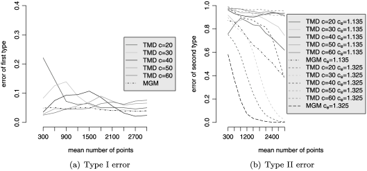
Figure 1: Empirical errors of types I and II for the TMD and the MGM test plotted against the mean number of points in the observation window ($\alpha=0.5$). The constant $c$ is a bandwidth parameter for covariance estimation in the TMD test, whereas $c_{e}$ denotes the elongation factor of ellipses forming the Boolean model used as input data for the analysis of type II errors.

The relatively high errors of second type for the small elongation factor of $c_{e}=1.135$ are to be expected, since the investigated structures are only slightly anisotropic. Nevertheless, for an expected number of $3000$ points the MGM and TMD tests achieve a power of $\sim 60\%$ and $40\%$, respectively, for $c_{e}=1.135$ and reject the null hypothesis with probabilty $1$ for $c_{e}=1.325$. In summary, our simulation results indicate that the MGM test outperforms the TMD test especially with respect to power. This result is plausible since the additional information incorporated into $H_{0}$ by specification of a model covariance matrix can be expected to result in a more specific test.

References

- [1] {barticle}[auto:STB—2013/06/05—13:45:01] \bauthor\bsnmBeneš, \bfnmV.\binitsV., \bauthor\bsnmHlawiczková, \bfnmM.\binitsM., \bauthor\bsnmGokhale, \bfnmA.\binitsA. &\bauthor\bsnmVander Voort, \bfnmG.\binitsG. (\byear2001). \btitleAnisotropy estimation properties for microstructural models. \bjournalMater. Charact. \bvolume46 \bpages93–98. \bptokimsref \endbibitem
- [2] {barticle}[mr] \bauthor\bsnmBöhm, \bfnmS.\binitsS. &\bauthor\bsnmSchmidt, \bfnmV.\binitsV. (\byear2004). \btitleAsymptotic properties of estimators for the volume fractions of jointly stationary random sets. \bjournalStat. Neerl. \bvolume58 \bpages388–406. \biddoi=10.1111/j.1467-9574.2004.00267.x, issn=0039-0402, mr=2106346 \bptokimsref \endbibitem
- [3] {bbook}[mr] \bauthor\bsnmBradley, \bfnmRichard C.\binitsR.C. (\byear2007). \btitleAn Introduction to Strong Mixing Conditions. Vols 1, 2, 3. \blocationHeber City, UT: \bpublisherKendrick Press. \bptokimsref \endbibitem
- [4] {bbook}[auto:STB—2013/06/05—13:45:01] \bauthor\bsnmDaley, \bfnmD.\binitsD. &\bauthor\bsnmVere-Jones, \bfnmD.\binitsD. (\byear2003/2008). \btitleAn Introduction to the Theory of Point Processes. Vols I, II, \bedition2nd ed. \blocationNew York: \bpublisherSpringer. \bptokimsref \endbibitem
- [5] {bbook}[mr] \bauthor\bsnmDoukhan, \bfnmPaul\binitsP. (\byear1994). \btitleMixing: Properties and Examples. \bseriesLecture Notes in Statistics \bvolume85. \blocationNew York: \bpublisherSpringer. \biddoi=10.1007/978-1-4612-2642-0, mr=1312160 \bptokimsref \endbibitem
- [6] {bbook}[mr] \bauthor\bsnmFolland, \bfnmGerald B.\binitsG.B. (\byear1999). \btitleReal Analysis: Modern Techniques and Their Applications, \bedition2nd ed. \bseriesPure and Applied Mathematics (New York). \blocationNew York: \bpublisherWiley. \bidmr=1681462 \bptokimsref \endbibitem
- [7] {barticle}[mr] \bauthor\bsnmGuan, \bfnmYongtao\binitsY., \bauthor\bsnmSherman, \bfnmMichael\binitsM. &\bauthor\bsnmCalvin, \bfnmJames A.\binitsJ.A. (\byear2004). \btitleA nonparametric test for spatial isotropy using subsampling. \bjournalJ. Amer. Statist. Assoc. \bvolume99 \bpages810–821. \biddoi=10.1198/016214504000001150, issn=0162-1459, mr=2090914 \bptokimsref \endbibitem
- [8] {barticle}[mr] \bauthor\bsnmGuan, \bfnmYongtao\binitsY., \bauthor\bsnmSherman, \bfnmMichael\binitsM. &\bauthor\bsnmCalvin, \bfnmJames A.\binitsJ.A. (\byear2007). \btitleOn asymptotic properties of the mark variogram estimator of a marked point process. \bjournalJ. Statist. Plann. Inference \bvolume137 \bpages148–161. \biddoi=10.1016/j.jspi.2005.10.004, issn=0378-3758, mr=2292847 \bptokimsref \endbibitem
- [9] {barticle}[mr] \bauthor\bsnmHeinrich, \bfnmLothar\binitsL. (\byear1994). \btitleNormal approximation for some mean-value estimates of absolutely regular tessellations. \bjournalMath. Methods Statist. \bvolume3 \bpages1–24. \bidissn=1066-5307, mr=1272628 \bptokimsref \endbibitem
- [10] {barticle}[auto:STB—2013/06/05—13:45:01] \bauthor\bsnmHeinrich, \bfnmL.\binitsL., \bauthor\bsnmKlein, \bfnmS.\binitsS. &\bauthor\bsnmMoser, \bfnmM.\binitsM. (\byear2014). \btitleEmpirical mark covariance and product density function of stationary marked point processes – A survey on asymptotic results. \bjournalMethodol. Comput. Appl. Probab. \bvolume16 \bpages283–293. \biddoi=10.1016/j.jspi.2005.10.00410.1007/s11009-012-9314-7,mr=3199047 \bptokimsref \endbibitem
- [11] {barticle}[auto:STB—2013/06/05—13:45:01] \bauthor\bsnmHeinrich, \bfnmL.\binitsL., \bauthor\bsnmLück, \bfnmS.\binitsS., \bauthor\bsnmNolde, \bfnmM.\binitsM. &\bauthor\bsnmSchmidt, \bfnmV.\binitsV. (\byear2014). \btitleOn strong mixing, Bernstein’s blocking method and a CLT for spatial marked point processes. \bjournalYokohama Math. J. \bnoteTo appear. \bptokimsref \endbibitem
- [12] {bmisc}[auto:STB—2013/06/05—13:45:01] \bauthor\bsnmHeinrich, \bfnmL.\binitsL., \bauthor\bsnmLück, \bfnmS.\binitsS. &\bauthor\bsnmSchmidt, \bfnmV.\binitsV. (\byear2012). \bhowpublishedNon-parametric asymptotic statistics for the Palm mark distribution of -mixing marked point processes. Available at \arxivurlarXiv:1205.5044v1 [math.ST]. \bptokimsref \endbibitem
- [13] {barticle}[mr] \bauthor\bsnmHeinrich, \bfnmLothar\binitsL. &\bauthor\bsnmMolchanov, \bfnmIlya S.\binitsI.S. (\byear1999). \btitleCentral limit theorem for a class of random measures associated with germ-grain models. \bjournalAdv. in Appl. Probab. \bvolume31 \bpages283–314. \biddoi=10.1239/aap/1029955136, issn=0001-8678, mr=1724553 \bptokimsref \endbibitem
- [14] {barticle}[mr] \bauthor\bsnmHeinrich, \bfnmLothar\binitsL. &\bauthor\bsnmPawlas, \bfnmZbyněk\binitsZ. (\byear2008). \btitleWeak and strong convergence of empirical distribution functions from germ-grain processes. \bjournalStatistics \bvolume42 \bpages49–65. \biddoi=10.1080/02331880701538531, issn=0233-1888, mr=2396675 \bptokimsref \endbibitem
- [15] {barticle}[mr] \bauthor\bsnmHeinrich, \bfnmLothar\binitsL. &\bauthor\bsnmProkešová, \bfnmMichaela\binitsM. (\byear2010). \btitleOn estimating the asymptotic variance of stationary point processes. \bjournalMethodol. Comput. Appl. Probab. \bvolume12 \bpages451–471. \biddoi=10.1007/s11009-008-9113-3, issn=1387-5841, mr=2665270 \bptokimsref \endbibitem
- [16] {bbook}[mr] \bauthor\bsnmKallenberg, \bfnmOlav\binitsO. (\byear1986). \btitleRandom Measures. \blocationLondon: \bpublisherAcademic Press. \bptokimsref \endbibitem
- [17] {barticle}[auto:STB—2013/06/05—13:45:01] \bauthor\bsnmLück, \bfnmS.\binitsS., \bauthor\bsnmKupsch, \bfnmA.\binitsA., \bauthor\bsnmLange, \bfnmA.\binitsA., \bauthor\bsnmHentschel, \bfnmM.\binitsM. &\bauthor\bsnmSchmidt, \bfnmV.\binitsV. (\byear2012). \btitleStatistical analysis of tomographic reconstruction algorithms by morphological image characteristics. \bjournalMater. Res. Soc. Symp. Proc. \bvolume1421. \bnoteDOI:\doiurl10.1557/opl.2012.209. \bptokimsref \endbibitem
- [18] {barticle}[pbm] \bauthor\bsnmMidgley, \bfnmP. A.\binitsP.A. &\bauthor\bsnmWeyland, \bfnmM.\binitsM. (\byear2003). \btitle3D electron microscopy in the physical sciences: The development of Z-contrast and EFTEM tomography. \bjournalUltramicroscopy \bvolume96 \bpages413–431. \biddoi=10.1016/S0304-3991(03)00105-0, issn=0304-3991, pii=S0304-3991(03)00105-0, pmid=12871805 \bptokimsref \endbibitem
- [19] {barticle}[mr] \bauthor\bsnmPawlas, \bfnmZbyněk\binitsZ. (\byear2009). \btitleEmpirical distributions in marked point processes. \bjournalStochastic Process. Appl. \bvolume119 \bpages4194–4209. \biddoi=10.1016/j.spa.2009.10.002, issn=0304-4149, mr=2565564 \bptokimsref \endbibitem
- [20] {bbook}[mr] \bauthor\bsnmSchneider, \bfnmRolf\binitsR. (\byear1993). \btitleConvex Bodies: The Brunn–Minkowski Theory. \bseriesEncyclopedia of Mathematics and Its Applications \bvolume44. \blocationCambridge: \bpublisherCambridge Univ. Press. \biddoi=10.1017/CBO9780511526282, mr=1216521 \bptokimsref \endbibitem
- [21] {barticle}[mr] \bauthor\bsnmYoshihara, \bfnmKen-Ichi\binitsK.I. (\byear1976). \btitleLimiting behavior of -statistics for stationary, absolutely regular processes. \bjournalZ. Wahrsch. Verw. Gebiete \bvolume35 \bpages237–252. \bidmr=0418179 \bptokimsref \endbibitem