POISSON project

Abstract

Context. As part of the POISSON project (Protostellar Optical-Infrared Spectral Survey on NTT), we present the results of the analysis of low-resolution near-IR spectroscopic data (0.9-2.4 $\mu$m) of two samples of young stellar objects in the Lupus (52 objects) and Serpens (17 objects) star-forming clouds, with masses in the range of 0.1 to 2.0 M_⊙ and ages spanning from 10⁵ to a few 10⁷ yr.

Aims. After determining the accretion parameters of the targets by analysing of their H i near-IR emission features, we added the results from the Lupus and Serpens clouds to those from previous regions (investigated in POISSON with the same methodology) to obtain a final catalogue (143 objects) of mass accretion rate values ($\dot{M}_{acc}$) derived in a homogeneous and consistent fashion. Our final goal is to analyse how $\dot{M}_{acc}$ correlates with the stellar mass ($M_{\mathrm{*}}$) and how it evolves in time in the whole POISSON sample.

Methods. We derived the accretion luminosity ($L_{\mathrm{acc}}$) and $\dot{M}_{acc}$ for Lupus and Serpens objects from the Br$\gamma$ (Pa$\beta$ in a few cases) line by using relevant empirical relationships available in the literature that connect H i line luminosity and $L_{\mathrm{acc}}$. To minimise the biases that arise from adopting literature data that are based on different evolutionary models and also for self-consistency, we re-derived mass and age for each source of the POISSON samples using the same set of evolutionary tracks.

Results. We observe a correlation $\dot{M}_{acc}$$\sim$$M_{\mathrm{*}}$^2.2 between mass accretion rate and stellar mass, similarly to what has previously been observed in several star-forming regions. We find that the time variation of $\dot{M}_{acc}$ is roughly consistent with the expected evolution of the accretion rate in viscous disks, with an asymptotic decay that behaves as $t^{-1.6}$. However, $\dot{M}_{acc}$ values are characterised by a large scatter at similar ages and are on average higher than the predictions of viscous models.

Conclusions. Although part of the scattering may be related to systematics due to the employed empirical relationship and to uncertainties on the single measurements, the general distribution and decay trend of the $\dot{M}_{acc}$ points are real. These findings might be indicative of a large variation in the initial mass of the disks, of fairly different viscous laws among disks, of varying accretion regimes, and of other mechanisms that add to the dissipation of the disks, such as photo-evaporation.

1 Introduction

A significant fraction of the mass of a star is accumulated by accretion from a circumstellar disk. After a short period of intense accretion, during which the star acquires most of its mass (the so-called Class 0 phase), the material continues to be channelled from the inner disk onto the central star along the stellar magnetic field lines. Although the rate of mass accretion decreases with time, this process plays a crucial role in removing material from the disk along with mass loss, and in this way it influences the disk dissipation time-scales and eventually the formation of planets.

The infalling material landing on the stellar surface produces strong shocks and creates a so-called hot spot, where the accretion luminosity ($L_{\mathrm{acc}}$) is radiatively released as continuum and line emission. Therefore, by observing this emission one can infer quantitative information on the stellar accretion process. In particular, $L_{\mathrm{acc}}$ can be directly measured for example by modelling the excess of UV continuum emission shortward of the Balmer and Paschen jumps (e.g. Calvet & Gullbring 1998). Mass accretion rates ($\dot{M}_{acc}$) can then be inferred from $L_{\mathrm{acc}}$  if the stellar mass and radius are known, in the assumption that the accretion energy is entirely converted into radiation. It has been found that accretion luminosity derived from the UV continuum excess obeys empirical relationships with several emission lines such as optical and IR hydrogen lines, CaII, and HeI (e.g. Herczeg & Hillenbrand 2008; Calvet et al. 2000, 2004). The discovery of these correlations has triggered a significant observational effort to measure the mass accretion rate of large populations of young stars, with the aim of defining its dependence on the stellar mass and its time evolution.

Following first observations concentrated on the population of the Taurus molecular cloud (e.g. Muzerolle et al. 1998; Herczeg & Hillenbrand 2008), recent studies have been conducted in other star-forming regions with the aim of addressing the dependence of mass accretion on the overall age of the stellar population and environment, such as in $\rho$ Oph (Natta et al. 2004), L1641 (Fang et al. 2009; Caratti o Garatti et al. 2012), Chamaeleon, (Antoniucci et al. 2011), $\sigma$ Ori (Rigliaco et al. 2011), and Lupus (Alcalá et al. 2014). These works have shown that there is a general dependence of $\dot{M}_{acc}$  on both the stellar mass and age, although with a large scatter. Some of the reasons for this scatter rely on accretion variability and uncertainty on the stellar parameters (especially the mass of the objects). A significant source of scatter also originates from the choice of tracers used to derive $\dot{M}_{acc}$ in the various studies, however. Indeed, accretion values measured on the same object may differ by more than one order of magnitude, which can be only partially justified by variability alone (e.g. Costigan et al. 2012). One way to reduce the biases induced by comparing $\dot{M}_{acc}$ values derived with different instrumentations and in different periods is to perform large spectroscopic surveys of young stars using (quasi)-simultaneous observations of tracers at different wavelengths (e.g Alcalá et al. 2014).

For the POISSON (Protostellar Objects IR-optical Spectral Survey On NTT) project, we have acquired optical/near-IR low-resolution spectra (R$\sim$700) of Spitzer-selected samples of sources in different nearby molecular clouds. In the first paper of the project (Antoniucci et al. 2011, hereafter Paper I) the $L_{\mathrm{acc}}$ of sources in the ChaI/II molecular clouds was derived from the line luminosity of several optical/IR tracers, and the different determinations were then compared. In the second paper (Caratti o Garatti et al. 2012, hereafter Paper II), a sample of young sources in the L1641 was characterised and their accretion properties were studied, addressing in particular the dependence of the accretion rate on the age.

The results so far obtained confirmed that some of the optical tracers commonly adopted to derive $L_{\mathrm{acc}}$ (e.g. H$\alpha$ and Ca II) present larger discrepancies than other lines, indicating that their luminosity might be contaminated by contributions in addition to the accretion, such as emission from jets and winds. Similar results were recently found by Rigliaco et al. (2012). Among the different tracers, we found that Br$\gamma$ and Pa$\beta$ luminosities provide the most reliable value for $L_{\mathrm{acc}}$in low-mass stars, because they require higher excitation conditions than other lines such as H$\alpha$, [O i], or Ca ii  and they are thus less likely to be contaminated by different contributions such as those coming from photosphere, winds, and jets. In addition, these near-infrared lines are less dependent on extinction than optical tracers and are particularly suited to derive the properties of younger and more embedded sources.

In the framework of the POISSON survey, we present here the near-infrared spectra (from 0.9 to 2.4$\mu$m) of two samples of young stellar objects (YSOs): one in Lupus (52 objects) and one in Serpens (17 sources). These clouds, which are located at a distance of 150-200 pc and 259 pc (see Comeron 2008; Straižys et al. 1996, 2003, and references therein), have been extensively investigated at various wavelengths in recent years: Hughes et al. (1994), Merín et al. (2008), Comerón et al. (2009), Mortier et al. (2011), Alcalá et al. (2014) for Lupus, and Winston et al. (2007, 2009), Gorlova et al. (2010) for Serpens. These works have provided information about the characterisation and properties of the young stellar population of these regions, which have been used in conjunction with the accretion luminosities and mass accretion rates, mostly derived from the Br$\gamma$ detected in emission in our spectra. By combining the Lupus and Serpens YSOs presented here with the previous samples of the POISSON survey, we obtain a general catalogue of 143 YSOs with accretion properties derived in an homogeneous way from near-IR lines.

The paper is structured as follows: in Sect. 2 we present the observations of the two samples of Lupus and Serpens and derive the accretion parameters of the sources in Sect. 3. Then, in Sect. 4 we consider the entire POISSON sample (five star-forming regions) and focus our attention on the temporal evolution of $\dot{M}_{acc}$ and on its dependence on the stellar mass. Our results are then discussed in Sects. 4.4 and 4.5. The main conclusions are summarised in Sect. 5.

Table 1: Observed Lupus targets and their main properties. All parameters are taken from the literature, except for $M_{\mathrm{*}}$, which was recomputed (see text).

ID	Name	RA	DEC	Other names	$L_{\mathrm{*}}$a	$T_{\mathrm{eff}}$a	$M_{\mathrm{*}}$a	$A_{V}$	$L^{b}_{\mathrm{disk}}$	$L_{\mathrm{bol}}$	ref.
		(2000)	(2000)		L⊙	K	M⊙	mag	L⊙	L⊙
LupIc
01	Sz65	15:39:27.77	-34:46:17.14	IK Lup	0.85	3800	0.52	0.2	1.01	1.86	2,4
02	Sz66	15:39:28.28	-34:46:18.03	[MJS2008] 6	0.20	3415	0.31	1.0	0.94	1.14	1,2
03	[MJS2008] 14	15:45:08.87	-34:17:33.34	…	0.70	4600	1.15	8.9	0.47	1.17	2,5
04	Sz68 A	15:45:12.86	-34:17:30.60	HT Lup	4.82	4955	2.00	1.5	0.66	5.48	2
05	Sz69	15:45:17.41	-34:18:28.33	HW Lup	0.09	3197	0.19	0.	0.35	0.44	1,2
06	[MJS2008] 17	15:45:18.52	-34:21:24.62	…	0.09	2700	0.06	1.6	0.01	0.10	2,5
07	Sz71	15:46:44.73	-34:30:35.50	GW Lup	0.31	3632	0.42	0.5	…	…	1
08	Sz72	15:47:50.62	-35:28:35.34	HM Lup	0.25	3560	0.38	0.75	…	…	1
09	Sz73	15:47:56.94	-35:14:34.66	HBC600	0.42	4060	0.80	3.5	…	…	1
10	Sz75	15:49:12.10	-35:39:05.12	GQ Lup	1.50	3900	0.59	0.95	…	…	4
LupIIc
11	Sz82	15:56:09.22	-37:56:05.78	IM Lup	1.29	3800	0.52	0.98	…	…	4
12	Sz83	15:56:42.30	-37:49:15.41	RU Lup	1.31	4060	0.74	0	…	…	1
13	Sz84	15:58:02.53	-37:36:02.69	…	0.12	3125	0.18	0	…	…	1
LupIVc
14	RY Lup	15:59:28.38	-40:21:51.30	…	1.26	4590	1.3	0.65	…	…	4
15	[MJS2008] 146	16:00:07.42	-41:49:48.42	IRAS15567-4141	2.74	2935	0.18	2	1.93	4.67	3
16	[MJS2008] 149	16:00:34.40	-42:25:38.62	…	1.45	2820	0.15	2	1.18	…	2
17	[HHC93] F403	16:00:44.53	-41:55:31.00	MY Lup,[MJS2008] 150	1.79	5152	1.39	0	0.17	…	2
18	EX Lup	16:03:05.49	-40:18:25.44	HD325367,HBC253	0.47	3802	0.53	3.1	…	…	3,6
19	Sz133	16:03:29.39	-41:40:01.83	…	0.36	4400	0.93	5.8	0.06	…	5
LupIIIc
20	Sz88 A	16:07:00.54	-39:02:19.30	HO Lup	0.49	3850	0.57	0.25	…	…	1
21	Sz88 B	16:07:00.62	-39:02:18.10	HO Lup B	0.12	3197	0.21	0	…	…	1
22	[MJS2008] 20	16:07:08.63	-39:47:21.90	…	0.30	4590	0.86	1	0.08	0.38	2
23	Sz90	16:07:10.07	-39:11:03.30	[KWS97] Lupus 3 23	1.10	3900	0.60	3.2	0.46	1.56	2,5
24	Sz95	16:07:52.30	-38:58:05.93	[MJS2008] 28	0.26	3400	0.31	0.7	0.07	0.33	2,5
25	[MJS2008] 36	16:08:06.18	-39:12:22.54	…	2.09	2935	0.18	5.3	0.61	2.7	3
26	Sz96	16:08:12.64	-39:08:33.48	[MJS2008] 37	0.82	3560	0.39	1.43	0.27	1.09	3
27	Sz97	16:08:21.80	-39:04:21.48	[MJS2008] 40	0.16	3270	0.25	0	0.06	0.22	1,3
28	Sz98	16:08:22.49	-39:04:46.46	HK Lup,V1279 Sco	2.35	4350	1.11	2.5	1.18	3.53	3
29	Sz99	16:08:24.04	-39:05:49.42	…	0.07	3270	0.21	0	0.07	0.14	1,3
30	Sz100	16:08:25.76	-39:06:01.19	[MJS2008] 43	0.17	3057	0.17	0	0.2	0.37	1,3
31	Sz103	16:08:30.27	-39:06:11.16	[MJS2008] 49	0.18	3270	0.25	0.7	0.08	0.26	1,3
32	[MJS2008] 50	16:08:30.70	-38:28:26.85	…	3.03	5000	1.79	1	0.65	3.68	2
33	Sz104	16:08:30.82	-39:05:48.87	…	0.10	3125	0.17	0	0.06	0.16	1,3
34	HR5999	16:08:34.28	-39:06:18.16	V856 Sco	48.3	7890	2.55	0.85	33.99	82.28	2,4
35	Sz106	16:08:39.76	-39:06:25.32	…	0.10	3777	0.51	1	0.11	0.21	1,2
36	Sz107	16:08:41.80	-39:01:37.02	[MJS2008] 58	0.15	2935	0.12	0	0.01	0.16	3
37	Sz109	16:08:48.16	-39:04:19.25	V1191 Sco	0.14	2800	0.09	0.2	0.06	0.20	2,5
38	[CFB2003] Par-Lup3-3	16:08:49.40	-39:05:39.34	…	0.23	3270	0.26	2.2	0.05	0.28	1,2
39	Sz110	16:08:51.57	-39:03:17.74	V1193 Sco,[MJS2008] 67	0.28	3270	0.27	0	0.07	0.35	1,3
40	[MJS2008] 68	16:08:53.24	-39:14:40.17	[G2006] 86	0.44	3900	0.62	3.3	-0.08d	0.36	2,5
41	Sz111	16:08:54.69	-39:37:43.11	Hen 3-1145,[MJS2008] 71	0.33	3750	0.50	0	0.2	0.53	1,2
42	Sz112	16:08:55.53	-39:02:33.95	[MJS2008] 73	0.19	3125	0.20	0	0.1	0.29	1,2
43	Sz113	16:08:57.80	-39:02:22.79	[MJS2008] 74	0.06	3197	0.17	1	0.09	0.15	1,3
44	Sz114	16:09:01.85	-39:05:12.42	[MJS2008] 80,V908 Sco	0.31	3175	0.23	0.3	0.4	0.71	1,3
45	Sz117	16:09:44.35	-39:13:30.10	[MJS2008] 102	0.47	3700	0.46	1.5	0	0.47	2,5
46	Sz118	16:09:48.65	-39:11:16.95	[MJS2008] 103	0.92	4060	0.75	2.6	0.56	1.48	3
47	[MJS2008] 113	16:10:18.58	-38:36:12.51	…	0.05	2900	0.09	0.2	0.03	0.08	2,5
48	[MJS2008] 114	16:10:19.85	-38:36:06.52	…	0.03	2990	0.09	0.4	0	0.03	3
49	Sz123	16:10:51.59	-38:53:13.77	[MJS2008] 121	0.20	3705	0.46	1.25	-0.01d	0.19	1,2
50	[MJS2008] 133	16:12:11.20	-38:32:19.74	…	1.00	4400	1.20	7	-0.27d	0.73	2,5
51	[MJS2008] 136	16:12:22.69	-37:13:27.65	…	2.87	5300	1.57	6	0.36	3.23	2
52	[MJS2008] 137	16:12:43.73	-38:15:03.15	…	0.60	4400	1.10	1	-0.01d	0.59	2,5

^a Typical relative uncertainties for the parameters are as follows (see text): $L_{\mathrm{*}}$ 40%, $T_{\mathrm{eff}}$ 20%, $M_{\mathrm{*}}$ 40%.
^b $L_{\mathrm{disk}}$ is computed as $L_{\mathrm{bol}}$– $L_{\mathrm{*}}$ (see Sect. 2.2).
^c Assumed sub-cloud distances are: 150 pc for Lup I, II, and IV and 200 pc for Lup III (Comeron 2008).
^d $L_{\mathrm{disk}}$ is assumed to be 0 in these sources because $L_{\mathrm{bol}}$–$L_{\mathrm{*}}$ gives a negative value (see text).
References. 1: Alcalá et al. (2014), 2: Merín et al. (2008), 3: Mortier et al. (2011), 4: Hughes et al. (1994), 5: Comerón et al. (2009), 6: Lorenzetti et al. (2012).

Table 2: Observed Serpens targets and their main properties. All parameters are taken from the literature, except for $M_{\mathrm{*}}$, which was recomputed (see text).

ID	Name	RA	DEC	Other Names	$L_{\mathrm{*}}$a	$T_{\mathrm{eff}}$a	$M_{\mathrm{*}}$a	$A_{V}$	$L^{b}_{\mathrm{disk}}$	$L_{\mathrm{bol}}$	ref.
.	.	(2000)	(2000)	.	L⊙	K	M⊙	mag	L⊙	L⊙
01	[WMW2007]103	18:29:41.472	01:07:37.90	…	1.37	4832	1.39	6.2	0.13	1.5	1,2
02	[WMW2007]65	18:29:43.932	01:07:20.80	…	0.21	4060	0.77	8.0	0.08	0.29	1,2
03	[WMW2007]7	18:29:49.602	01:17:05.83	EC76	1.90	3400	0.32	9.6	-0.8c	1.1	1,4
04	[WMW2007]81	18:29:53.608	01:17:01.73	EC67	0.48	3560	0.38	7.4	0.31	0.79	1,2
05	[WMW2007]38	18:29:55.711	01:14:31.50	GEL4,EC74	1.00	3199	0.24	18.5d	0.2	1.2	1,3
06	[WMW2007]80	18:29:56.553	01:12:59.65	GEL5,SVS4-2,EC79	0.49	…	…	14.2	0.1	0.59	1,3
07	[WMW2007]85	18:29:56.967	01:12:47.83	EC84	2.00	2965	0.18	19.4d	…	…	2,3
08	[WMW2007]35	18:29:57.737	01:14:05.69	GEL10,EC90	0.27	3270	0.26	9.6	47.73	48	1,5
09	[WMW2007]83	18:29:57.816	01:15:31.86	CK13,EC93	4.40	4900	2.00	24.4d	-1.6c	2.8	1,2
10	[WMW2007]70	18:29:57.819	01:12:28.05	[ACA2003]SerA4,EC91	1.00	3600	0.40	40.0d	0.8	1.8	1,4
11	[WMW2007]37	18:29:57.849	01:12:37.90	EC94	4.30	4000	0.70	40.0d	1.8	6.1	1,4
12	[WMW2007]2	18:29:57.858	01:12:51.40	EC92	…	…	…	9.6	…	4.8	1
13	[WMW2007]27	18:29:58.205	01:15:21.68	GEL12,CK4,EC97	0.96	3997	0.69	12.8	1.64	2.6	1,2
14	[WMW2007]4	18:29:58.765	01:14:25.78	EC103	…	…	…	9.6	…	1.6	1
15	[WMW2007]10	18:30:02.747	01:12:28.06	EC129	9.50	3872	0.68	24.0d	-3.7c	5.8	1,3
16	[WMW2007]78	18:30:03.413	01:16:19.14	EC135	0.54	3850	0.57	5.9	0.2	0.74	1,2
17	[WMW2007]73	18:30:07.708	01:12:04.32	…	0.78	3487	0.35	7.4	0.42	1.2	1,2

Assumed distance is 259 pc (Straižys et al. 1996).
^a Typical relative uncertainties for the parameters are as follows (see text): $L_{\mathrm{*}}$ 40%, $T_{\mathrm{eff}}$ 20%, $M_{\mathrm{*}}$ 40%.
^b $L_{\mathrm{disk}}$ is computed as $L_{\mathrm{bol}}$– $L_{\mathrm{*}}$ (see Sect. 2.2).
^c $L_{\mathrm{disk}}$ is assumed to be 0 in these sources because $L_{\mathrm{bol}}$–$L_{\mathrm{*}}$ gives a negative value.
^d For these high-extinction objects the stellar parameters must be considered to be less reliable.
References. 1: Evans et al. (2009), 2: Winston et al. (2007, 2009), 3: Gorlova et al. (2010), 4: Doppmann et al. (2005), 5: Oliveira et al. (2009).

2 Lupus and Serpens observations

2.1 Sample selection

Analogously to previous star-forming clouds analysed by POISSON (paper I and II), most of the targets in Lupus and Serpens were chosen from the young populations of ClassI/II objects identified through Spitzer surveys.

We used the works by Merín et al. (2008) and Winston et al. (2007, 2009) as the main reference articles to select Lupus and Serpens targets. We selected sources with a $K$-band magnitude $\lesssim$ 12 mag (which was basically imposed by the sensitivity offered by La Silla instruments) and with a spectral energy distribution (SED) spectral index between 2 and 24 $\mu$m $\alpha_{2-24}\gtrsim-1.6$, so as to include the Class II sources as classically defined by Lada & Wilking (1984) (see also Greene et al. 1994). A few sources with $-1.6<\alpha_{2-24}<-1.9$ or $K$-band magnitude $>$ 12 mag, which were located very close to selected targets, were observed with the same slit acquisition and were eventually included in the sample. By using these selection criteria, which were chosen to also ensure a high detection rate for H i lines, we initially selected 60 objects in Lupus and 30 objects in Serpens, of which we eventually observed 43 in Lupus and 17 in Serpens. Finally, we added to the sample nine bright T Tauri objects in Lupus with known disks, taken from the sample of van Kempen et al. (2007), which were not present in the list of Merín et al. (2008). The final sample consists of 52 (17) sources in Lupus (Serpens), namely: 1 (3) Class I, 3 (2) flat, and 48 (12) Class II.

Almost all sources in Lupus are Class II objects, consistent with the relatively old average age of 3-4 Myr estimated for the Lupus YSOs (Hughes et al. 1994; Mortier et al. 2011). The percentage of younger Class I/flat sources is somewhat higher in the Serpens sample, in general agreement with the younger mean age of 1-3 Myr of the Serpens association recently found by a few works (Winston et al. 2009; Gorlova et al. 2010). However, these works also reported multiple young stellar populations in the cloud.

The complete list of targets is presented in Tables 1 and 2.

2.2 Source parameters

All relevant stellar parameters of the investigated objects ($L_{\mathrm{*}}$, $T_{\mathrm{eff}}$, visual extinction, disk luminosity $L_{\mathrm{disk}}$, and bolometric luminosity $L_{\mathrm{bol}}$) were taken from the literature and are reported in Tables 1 and 2 together with all the references used. As a general rule, when more than one literature value was available for a given parameter, we adopted the most recent determination, using the observed dispersion of values to estimate the average uncertainty on that parameter in our sources.

The mean uncertainty on the adopted $L_{\mathrm{*}}$ is a factor 1.4, corresponding to 0.1-0.2 L_⊙ for the lowest luminosity objects ($L_{\mathrm{*}}$$<$0.7 L_⊙). The typical error on the determination of the spectral type is 1-2 spectral sub-classes, which means an uncertainty of a factor 1.1-1.2 for the $T_{\mathrm{eff}}$ of the sources.

The reported $L_{\mathrm{disk}}$ is an estimate of the luminosity of the circumstellar disk and was simply computed as the difference between the total luminosity of the object $L_{\mathrm{bol}}$ and the stellar luminosity $L_{\mathrm{*}}$ ($L_{\mathrm{disk}}$$=$$L_{\mathrm{bol}}$$-$$L_{\mathrm{*}}$). In a few sources we obtained a negative value of $L_{\mathrm{disk}}$, because $L_{\mathrm{bol}}$ and $L_{\mathrm{*}}$ values are often independent determinations from different works (inferred by integrating the spectral energy distribution and by spectral type fitting). In these cases, the derived $L_{\mathrm{disk}}$ is in general a small fraction of $L_{\mathrm{*}}$, so we assume that $L_{\mathrm{disk}}$ is negligible ($\sim 0$ L_⊙) in these objects.

For stellar masses ($M_{\mathrm{*}}$), the values derived from the position on the HR diagram ($L_{\mathrm{*}}$ and $T_{\mathrm{eff}}$ values, see Fig. 9) were preferred to the ones found in literature. With this aim, we used the pre-main sequence tracks computed by Siess et al. (2000), to minimise biases due to the adoption of different pre-main sequence evolutionary models in the reference articles. Details about $M_{\mathrm{*}}$ computation are given in Sect. 4.1 and in the appendix. The relative error on the mass value can be estimated from the uncertainties on $L_{\mathrm{*}}$ and $T_{\mathrm{eff}}$, and is typically 30-40%. All sources in both clouds have masses ranging between 0.1 and 2.0 M_⊙ and present late spectral types, from K to late M, with the exception of HR 5999 in Lupus, which appears as an Herbig A6e star of about 2.5M_⊙.

2.3 Extinction

Lupus objects present fairly low visual extinction values ($<$$A_{V}$$>$=1.5 mag), while sources in Serpens are on average more embedded, with $<$$A_{V}$$>=17$ mag. For Lupus we assumed a mean uncertainty on the extinction of 0.5 mag (note that many sources have $A_{V}$ values in the range 0-0.5 mag). For the more embedded Serpens objects, we considered an $A_{V}$ mean uncertainty of 1 mag, but assumed a highly conservative uncertainty of 4 mag for the six objects with $A_{V}$$\gtrsim$20 mag. We considered these uncertainties in computing the accretion parameters (see Sect. 3). Because of the large $A_{V}$ uncertainty of the high-extinction sources (only four with accretion determinations), the literature stellar parameters (especially $L_{\mathrm{*}}$) must be considered less reliable. In this work we employed the extinction law parametrisation by Cardelli et al. (1989), adopting a value of the total-to-selective extinction ratio $R_{V}$=5.5 for both star-forming clouds. We used this law to compute (from the provided $A_{V}$) the extinction at the wavelength of the Pa$\beta$ and Br$\gamma$ lines (i.e. $A_{J}$ and $A_{K}$), which we considered to derive the accretion luminosity (see Sect 4.2). Using instead a standard interstellar extinction law like that of Rieke & Lebofsky (1985) to convert $A_{V}$ would result in a variation of about 20% of the value of $A_{J}$ and $A_{K}$ we obtained from Cardelli’s law.

2.4 Observations and data reduction

Observations were carried out at ESO La Silla on 8-11 July 2009 with SofI (Morwood 1997; D’Odorico 1988) mounted on the NTT (Tarenghi & Wilson 1989). We used the red and blue grisms (hereafter RG and BG) of SofI, combined with the 0$\aas@@fstack{\prime\prime}$6 slit, which provides a final resolution R $\sim$ 900 in the 0.9-2.4 $\mu$m  wavelength range (0.94–1.65 $\mu$m the BG, 1.50–2.40 $\mu$m the RG). The two grisms were acquired in succession, so that BG and RG spectra can be considered as taken almost simultaneously. EFOSC2 optical observations of the targets were programmed but could not be performed because of bad weather conditions.

The RG and BG spectra are available for all Lupus sources. As for Serpens, we acquired the RG spectrum for all objects, while the BG was taken only for four sources, which were sufficiently bright ($J\lesssim$14 mag).

All data were reduced using the IRAF software package. We followed the standard procedures for bad pixel removal, flat-fielding, and sky subtraction. Spectra of standard stars were acquired at air-masses similar to those of the targets and used, after removal of any intrinsic line, to correct the scientific spectra for telluric absorption and calibrate the instrumental response. Wavelength calibration for all spectra was obtained using xenon-argon arc lamps.

In addition to spectroscopic data, $H$-band photometry was obtained within 24 hours from the spectral observations for all sources but HR 5999 (see Tables in appendix). The measured magnitudes were employed to flux-calibrate each RG spectrum at the effective wavelength of the SofI $H$ filter. 2MASS (Skrutskie et al. 2006) $H$ magnitude was instead used to flux-calibrate the RG spectrum of HR 5999. The BG spectrum (when available) was then re-scaled to match the corresponding RG spectrum over the spectral region where the two segments overlap.

From the flux-calibrated spectra we finally derived $J$- and $K$-band magnitudes by measuring the specific flux at the effective wavelengths of the relative Johnson filters (1.25 $\mu$m for $J$ and 2.20 $\mu$m for $K$). We estimate a typical uncertainty of 0.05 mag for our $H$ photometry measurements and a more conservative uncertainty of 0.1 mag for the $J$- and $K$-band magnitudes, to take into account possible errors on the derived instrument response function. These values translate into a flux calibration relative error of about 10%, which we assumed for our spectra. Our photometric results are compared with 2MASS in appendix A for the identification of variable sources.

2.5 Spectra

Some example spectra are shown in Fig. 10 in the Appendix. H i recombination lines in emission from the Paschen and Brackett series are the most prominent features detected in the spectra, in particular the Br$\gamma$ and Pa$\beta$ lines, which remain unresolved given the low spectral resolution of the observations. At least one of these two lines is detected in 30 ($\sim$58% of the total) sources in Lupus and 8 ($\sim$47%) in Serpens. The only other permitted feature observed is the He i line at 1.08$\mu$m(19 sources in Lupus), which is a common tracer of winds from the young stars (e.g. Edwards et al. 2006). Consistently with this origin, we observe an evident P Cygni signature in at least three objects of Lupus.

The detection rates of near-IR H i lines are lower than in clouds investigated in paper I and II with the same instruments and modalities, but are consistent with the Lupus sample being older and Serpens objects being on average more extincted. Noticeably, as already found for the Cha I and Cha II samples of paper I, forbidden emission lines usually taken as indicators of ejection activity (see e.g. Nisini et al. 2005b; Podio et al. 2006) are not detected in any object. Similarly, molecular transitions of H₂, which is another tracer of shocks induced by outflowing matter, are detected only in one object of each sample. This lack of jet-line features is probably ascribable more to the low-resolution and relatively low-sensitivity of our observations than to an actual absence of jets from the sources (see Sect. 5 of paper I for a discussion on the sensitivity of the POISSON datasets).

In Tables 3 and 4 the fluxes of the Br$\gamma$ and Pa$\beta$ lines used to derive the accretion luminosity (see Sect. 4.2) are given, providing upper limits for non-detections and indicating for each source other emission features at the 3$\sigma$ level.

3 Accretion in Lupus and Serpens

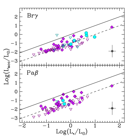
Figure 1: $L_{\mathrm{acc}}$ values derived from Br$\gamma$ and Pa$\beta$ for Lupus (purple diamonds) and Serpens (cyan circles) sources plotted as a function of $L_{\mathrm{*}}$. Downward triangles indicate upper limits on $L_{\mathrm{acc}}$. The solid and dashed lines show the locus where $L_{\mathrm{acc}}$=$L_{\mathrm{*}}$  and $L_{\mathrm{acc}}$=0.1$L_{\mathrm{*}}$. The mean uncertainty on the single points is also shown.

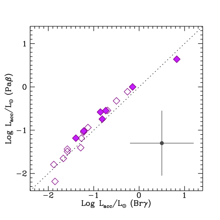
Figure 2: Comparison between $L_{\mathrm{acc}}$ determinations from Br$\gamma$ and Pa$\beta$ for Lupus objects in which both lines are detected. Filled symbols refer to stars with spectral type earlier than M0. The dashed line marks the locus of equal accretion luminosity.

Table 3: H i lines and derived accretion parameters for Lupus targets.

ID	Pa$\beta$		Br$\gamma$		$L_{\mathrm{acc}}$(Pa$\beta$)a	$L_{\mathrm{acc}}$(Br$\gamma$)a	$\dot{M}_{acc}$(Br$\gamma$)a	other linesb
	(F $\pm$ $\Delta$ F)10-14	EW	(F $\pm$ $\Delta$ F)10-14	EW			10-9
	erg s-1 cm-2	Å	erg s-1 cm-2	Å	L⊙	L⊙	M⊙ yr-1
01	$<$ 11	…	$<$ 3.7	…	$<$ 0.04	$<$ 0.06	$<$9.9
02	1.5 $\pm$ 0.4	-0.7	0.7 $\pm$ 0.2	-0.7	0.01	0.01	2.3
03	5.4 $\pm$ 0.3	-9.5	3.1 $\pm$ 0.3	-6.3	0.25	0.14	6.3	He i
04	$<$ 47	…	$<$ 16	…	$<$ 0.26	$<$ 0.26	$<$15
05	4.9 $\pm$ 0.6	-3.5	0.7 $\pm$ 0.2	-1.0	0.02	0.01	2.7
06	$<$ 0.54	…	$<$ 0.4	…	$<$ 0.01	$<$ 0.01	$<$9.5
07	5.6 $\pm$ 1.4	-2.3	$<$ 2.3	…	0.02	$<$ 0.04	2.8c	He i
08	9.5 $\pm$ 0.5	-6.3	2.9 $\pm$ 0.3	-4.6	0.04	0.05	7.1	He i
09	18.0 $\pm$ 1.4	-12.2	6.9 $\pm$ 0.9	-5.2	0.18	0.15	10	He i
10	61.0 $\pm$ 6.0	-4.3	12.0 $\pm$ 3.8	-1.4	0.28	0.18	34	He i(PC)
11	$<$ 16	…	$<$ 10	…	$<$ 0.07	$<$ 0.16	$<$33
12	270.0 $\pm$4.2	-26.1	59.0 $\pm$ 2.9	-9.3	1.00	0.72	90	He i
13	$<$ 1.9	…	0.9 $\pm$ 0.2	-2.0	$<$ 0.01	0.02	4.3
14	11.0 $\pm$ 2.7	-0.7	$<$ 11	…	0.04	$<$ 0.17	2.4c
15	120.0 $\pm$6.6	-3.2	34 $\pm$ 10	-1.7	0.76	0.55	780
16	45.0 $\pm$ 1.8	-5.0	1.1 $\pm$ 1.7	-2.2	0.28	0.20	270
17	$<$ 12	…	$<$ 2.8	…	$<$ 0.04	$<$ 0.05	$<$2.2
18	11.0$\pm$ 1.4	-2.5	2.5 $\pm$ 0.6	-2.0	0.09	0.06	7.1	He i
19	1.7 $\pm$ 0.2	-2.8	$<$ 0.9	…	0.03	$<$ 0.03	1.4c	He i
20	69.0 $\pm$ 1.7	-20.3	13.0 $\pm$ 0.7	-8.6	0.47	0.32	35	He i
21	0.65 $\pm$ 0.2	-0.7	$<$ 0.5	…	0.00	$<$ 0.02	0.8c
22	$<$ 1.3	…	$<$ 0.5	…	$<$ 0.01	$<$ 0.02	$<$0.7
23	4.2 $\pm$ 0.7	-2.2	0.9 $\pm$ 0.2	-0.8	0.06	0.04	6.2	He i(PC)
24	$<$ 1.8	…	$<$ 0.6	…	$<$ 0.01	$<$ 0.02	$<$3.8
25	$<$ 4.4	…	$<$ 5.7	…	$<$ 0.13	$<$ 0.26	$<$330
26	3.4 $\pm$ 0.8	-1.5	$<$ 1.2	…	0.03	$<$ 0.04	7.5c
27	$<$ 1.6	…	$<$ 0.6	…	$<$ 0.01	$<$ 0.02	$<$4.2
28	4.9 $\pm$ 0.6	-3.0	$<$ 2.0	…	0.06	$<$ 0.08	5.9c	He i
29	1.9 $\pm$ 0.3	-3.3	$<$ 0.4	…	0.01	$<$ 0.01	1.8c
30	$<$ 1.9	…	$<$ 0.6	…	$<$ 0.01	$<$ 0.02	$<$6.7
31	$<$ 1.2	…	$<$ 0.5	…	$<$ 0.01	$<$ 0.02	$<$3.6
32	$<$ 14	…	$<$ 3.9	…	$<$ 0.12	$<$ 0.12	$<$6.1
33	$<$ 1.1	…	$<$ 0.5	…	$<$ 0.01	$<$ 0.02	$<$4.0
34	500 $\pm$ 78	-4.5	45 $\pm$ 10	-0.6	4.33	6.73d	380d	He i
35	$<$ 1.1	…	0.3 $\pm$ 0.1	-0.7	$<$ 0.01	0.01	0.6	He i, H2
36	$<$ 2.1	…	$<$ 0.5	…	$<$ 0.01	$<$ 0.02	$<$8.2
37	$<$ 0.81	…	$<$ 0.4	…	$<$ 0.01	$<$ 0.02	$<$4.4
38	$<$ 0.77	…	$<$ 0.5	…	$<$ 0.01	$<$ 0.02	$<$5.2
39	6.2 $\pm$ 0.6	-4.6	0.8 $\pm$ 0.1	-1.8	0.04	0.03	4.8	He i
40	$<$ 1.1	…	0.3 $\pm$ 0.1	-0.8	$<$ 0.02	0.02	1.6
41	5.5 $\pm$ 0.6	-2.9	0.8 $\pm$ 0.2	-1.4	0.03	0.03	2.9	He i
42	$<$ 1.8	…	$<$ 1.0	…	$<$ 0.01	$<$ 0.03	$<$9.2
43	2.8 $\pm$ 0.2	-9.1	0.6 $\pm$ 0.1	-4.2	0.02	0.02	3.9	He i
44	9.9 $\pm$ 1.0	-4.5	1.8 $\pm$ 0.4	-2.3	0.07	0.05	17	He i
45	$<$ 2.4	…	$<$ 1.1	…	$<$ 0.02	$<$ 0.04	$<$5.6
46	7.3 $\pm$ 0.7	-3.5	1.5 $\pm$ 0.5	-1.2	0.09	0.06	6.2
47	$<$ 0.32	…	$<$ 0.2	…	$<$ 0.01	$<$ 0.01	$<$3.1	He i(PC)
48	$<$ 0.22	…	$<$ 0.1	…	$<$ 0.01	$<$ 0.01	$<$1.5
49	13.0 $\pm$ 0.5	-10.9	2.3 $\pm$ 0.2	-4.6	0.11	0.07	7.0	He i
50	$<$ 0.23	…	$<$ 0.2	…	$<$ 0.01	$<$ 0.02	$<$1.2
51	5.3 $\pm$ 0.4	-2.7	$<$ 1.7	…	0.18	$<$ 0.10	9.4c
52	$<$ 2.6	…	$<$ 1.1	…	$<$ 0.02	$<$ 0.04	$<$1.8

^a Typical uncertainties on $L_{\mathrm{acc}}$ and $\dot{M}_{acc}$ is 0.7 dex and 0.8 dex.
^b P Cygni profiles are indicated with PC.
^c $\dot{M}_{acc}$ value computed from Pa$\beta$.
^d Value obtained considering correction for Br$\gamma$ photospheric absorption (see text).

Table 4: H i lines and derived accretion parameters for Serpens targets.

ID	Pa$\beta$		Br$\gamma$		$L_{\mathrm{acc}}$(Pa$\beta$)a	$L_{\mathrm{acc}}$(Br$\gamma$)a	$\dot{M}_{acc}$(Br$\gamma$)a	other lines
	(F $\pm$ $\Delta$ F)10-14	EW	(F $\pm$ $\Delta$ F)10-14	EW			10-9
	erg s-1 cm-2	Å	erg s-1 cm-2	Å	L⊙	L⊙	M⊙ yr-1
01	…	…	2.2 $\pm$ 0.1	-3.5	…	0.20	9.7
02	…	…	$<$ 0.1	…	…	$<$ 0.02	$<$0.8
03	…	…	$<$ 0.2	…	…	$<$ 0.04	$<$19
04	1.1 $\pm$ 0.2	-4.0	$<$ 0.3	…	0.09	$<$ 0.04	18b
05	…	…	0.20 $\pm$ 0.06	-1.3	…	0.08	40
06	…	…	$<$ 0.2	…	…	$<$ 0.05	…
07	…	…	$<$ 0.3	…	…	$<$ 0.2	$<$180
08	$<$ 0.5	…	$<$ 7.3	…	$<$0.08	$<$ 0.8	$<$210
09	…	…	1.0 $\pm$ 0.3	-6.8	…	0.74	43
10	…	…	$<$ 8.4	…	…	$<$ 0.01	$<$0.03
11	…	…	0.30 $\pm$ 0.06	-2.6	…	1.32	320
12	…	…	$<$ 0.4	…	…	$<$ 0.06	…
13	…	…	$<$ 2.3	…	…	$<$ 0.43	$<$51
14	…	…	0.20 $\pm$ 0.02	-5.0	…	0.03	…	H2
15	…	…	0.7 $\pm$ 0.06	-1.8	…	0.49	200
16	0.7 $\pm$ 0.2	-1.8	$<$ 0.7	…	0.04	$<$ 0.07	4.4b
17	$<$ 0.4	…	$<$0.7	…	$<$0.03	$<$ 0.07	$<$19

^a Typical uncertainties on $L_{\mathrm{acc}}$ and $\dot{M}_{acc}$ is 0.7 dex and 0.8 dex.
^b $\dot{M}_{acc}$ value computed from Pa$\beta$.

3.1 Accretion luminosities

Consistently with previous POISSON papers, we derived the accretion luminosity ($L_{\mathrm{acc}}$) from H i lines using the empirical relationships provided by Calvet et al. (2000, 2004), which connect the Br$\gamma$ (or Pa$\beta$) luminosities to $L_{\mathrm{acc}}$:

$$\mathrm{Log}\;L_{acc}/L_{\odot}=0.9\cdot\mathrm{Log}\;L_{\mathrm{Br\gamma}}/L_{\odot}+2.9\leavevmode\nobreak\ ,$$ (1)

$$\mathrm{Log}\;L_{acc}/L_{\odot}=1.03\cdot\mathrm{Log}\;L_{\mathrm{Pa\beta}}/L_{\odot}+2.8\leavevmode\nobreak\ .$$ (2)

The H i line luminosities were computed from measured fluxes corrected for extinction. The $L_{\mathrm{acc}}$ values inferred from the above relationships are listed in Tables 3 and 4, where we also provide upper limits (3$\sigma$) for non-detections. We discuss in Sect. 4.4 how these results vary by adopting other empirical relationships available in the literature.

In Fig. 1 we plot $L_{\mathrm{acc}}$ determinations from Br$\gamma$ and Pa$\beta$ as a function of the stellar luminosity $L_{\mathrm{*}}$. As for previously investigated samples (paper I and II), the plots show that $L_{\mathrm{acc}}$ is correlated with $L_{\mathrm{*}}$ and that the accretion luminosity is only a fraction of the stellar luminosity (as expected for Class II objects), with 0.1 $L_{\mathrm{*}}$$<$ $L_{\mathrm{acc}}$$<$ $L_{\mathrm{*}}$ for most sources, except for a few low accretors (0.01 $L_{\mathrm{*}}$$<$ $L_{\mathrm{acc}}$$<$ 0.1 $L_{\mathrm{*}}$) found in particular in Lupus.

For consistency with the procedure employed in paper I (see discussion in Sect. 6 therein), in this work we adopt $L_{\mathrm{acc}}$ values (and upper limits) computed from the luminosity of Br$\gamma$. We remark that we did not take into account the stellar photospheric absorption for the lines, whose contribution to Br$\gamma$ is negligible for late spectral types. The only exception is the source HR5999 in Lupus (spectral type A6), for which we computed the flux correction on the basis of the Br$\gamma$ absorption observed in a template spectrum of the same spectral type (for details see Garcia Lopez et al. 2011). The accretion luminosities were derived from Pa$\beta$ only for those sources where Br$\gamma$ is not detected (eight objects in Lupus and two in Serpens, see Tables 3 and 4). Neglecting photospheric absorption of Pa$\beta$ for stars earlier than M0 might lead to underestimate line fluxes (and hence accretion rates), this affects four of the eight sources of Lupus with $L_{\mathrm{acc}}$ derived from Pa$\beta$. For sources where both lines are observed (only 19 sources in Lupus) a direct comparison between the two $L_{\mathrm{acc}}$ from Br$\gamma$ and Pa$\beta$ shows that the values agree well within uncertainties on $L_{\mathrm{acc}}$ values, also in objects with spectral types earlier than M0, as displayed in Fig. 2. At variance with Cha I and Cha II results (see Fig. 4 in paper I), in Lupus objects we therefore find no evidence of sources for which Pa$\beta$ provides $L_{\mathrm{acc}}$ values significantly underestimated with respect to Br$\gamma$. Accordingly, measured intrinsic Pa$\beta$/Br$\gamma$ ratios are similar to those observed in Taurus (Pa$\beta$/Br$\gamma$ $\gtrsim 3$, Muzerolle et al. 1998).

The error on the derived $L_{\mathrm{acc}}$ values depends on the errors on both line flux and extinction, but it is largely dominated by the uncertainty on the parameters of the empirical relationships employed, so that we estimate it to be about 0.7 dex.

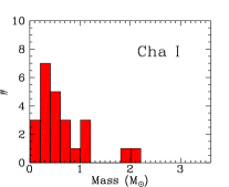
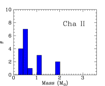
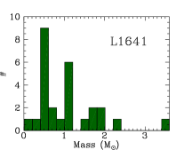
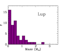
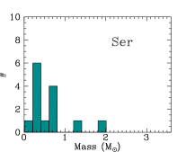
Figure 3: Histograms of stellar masses for the five samples investigated by POISSON.

3.2 Mass accretion rates

From the accretion luminosity $L_{\mathrm{acc}}$ we computed the mass accretion rate ($\dot{M}_{acc}$) by using the relationship (e.g. Gullbring et al. 1998)

$$\dot{M}_{acc}=\frac{L_{acc}R_{*}}{GM_{*}}\left(1-\frac{R_{*}}{R_{in}}\right)^{-1}\leavevmode\nobreak\ ,$$ (3)

where $M_{\mathrm{*}}$ and $R_{\mathrm{*}}$ are the stellar mass and radius, and $R_{in}$ is the inner truncation radius of the disk, which we assumed equal to $5R_{*}$. Mass estimates were derived as explained in Sect. 4.1 and the appendix, while $R_{\mathrm{*}}$ was calculated from $L_{\mathrm{*}}$ and $T_{\mathrm{eff}}$ listed in Tables 1 and 2:

$$R_{*}=\sqrt{L_{*}/4\pi\sigma T_{\mathrm{eff}}^{4}}\leavevmode\nobreak\ .$$ (4)

The $\dot{M}_{acc}$ values thus obtained are reported in Tables 3 and 4 for Lupus and Serpens. These are about 10^-8-10^-9 M_⊙ yr^-1for all objects, except for five sources displaying $\dot{M}_{acc}$$\sim$10^-7 M_⊙ yr^-1(three in Lupus and two in Serpens). We remark that two of the objects in Lupus are HR5999 (a Herbig star for which a higher accretion rate is expected) and [MJS2008] 146, which conversely is a low-mass source (0.18 M_⊙) that appears to be in an enhanced phase of accretion (see below). The inferred rates are in the range of values commonly observed in many Class II objects (see e.g. paper I, Gullbring et al. 1998; Natta et al. 2006; White et al. 2007). Considering the uncertainties on $L_{\mathrm{acc}}$ and $M_{\mathrm{*}}$, and assuming an additional typical 30% error on $R_{\mathrm{*}}$, we derive a relative error on the accretion rates of about 0.8 dex.

Mass accretion rates for several Lupus sources of our sample were recently inferred by Mortier et al. (2011) from the analysis of VLT/FLAMES spectra and by Alcalá et al. (2014) from VLT/X-Shooter data. Alcalá et al. (2014) observed 22 objects of our Lupus sample and derived $\dot{M}_{acc}$ estimates on the basis of the detected Balmer jump. The authors also measured the flux of several emission lines in the optical-NIR range (including Br$\gamma$ and Pa$\beta$) and used these results to provide new calibrated $L_{\mathrm{acc}}$-line relationships. From examining their Br$\gamma$ fluxes, we find a reasonable agreement with our measurements because fluxes differ by a factor lower than 3 in almost all objects. Albeit the fluxes are similar, the $\dot{M}_{acc}$ we eventually obtain appears to be on average higher than those derived in Alcalá et al. (2014) because of the $L_{\mathrm{acc}}$-Br$\gamma$ flux relationship we employed (see discussion in Sect. 4.4).

Mortier et al. (2011) give $\dot{M}_{acc}$ based on H$\alpha$ flux and width for 14 sources of our Lupus sample and seven for which we have a Br$\gamma$ detection. Our $\dot{M}_{acc}$ are very similar only for three of these sources, while they are significantly different for the others, with two targets showing a discrepancy exceeding 2 orders of magnitude.

Analogously, in eight sources in common between Mortier et al. and Alcalá et al., we find that in three cases their $\dot{M}_{acc}$ determinations differ by more than one order of magnitude. These fluctuations are similar to those observed in paper I for $L_{\mathrm{acc}}$ values derived from H$\alpha$, which we judged as the less reliable tracer. Indeed, $L_{\mathrm{acc}}$ determinations based on H$\alpha$ were characterised by a scatter two orders of magnitude greater than those from Br$\gamma$, most likely due to different emission components contributing to the line flux (see paper I).

For [MJS2008] 146, we measure an accretion rate about four orders of magnitude higher than Mortier et al., although using a different tracer. This enormous variation suggests that this object undergoes phases of outburst and quiescence, and as such it appears to be a good EXor candidate (e.g. Lorenzetti et al. 2012; Antoniucci et al. 2013a). This interpretation is also supported by the significant variation in magnitude with respect to 2MASS ($\Delta J\sim 1$ mag), which we signalled in Appendix A.

For Serpens sources no previous $\dot{M}_{acc}$ determinations were available in the literature.

Table 5: Number of observed objects compared with the total number of YSOs in the five samples of POISSON, with upper and lower limits of $M_{\mathrm{*}}$.

Region	total # of Class I/II YSOsa	observed	$M_{\mathrm{*}}$ range (M⊙)
Chamaeleon I	108	30	0.2–2.0
Chamaeleon II	26	17	0.2–1.9
L1641	$\sim$200	27	0.2–3.5
Lupus	95	52	0.1–2.0
Serpens	117	17	0.2–2.6

^a Estimates of the number of YSOs in the clouds are taken from Luhman (2007, ChaI), Alcalá et al. (2008, ChaII), Allen & Davis (2008, L1641), Evans et al. (2009, Lup, Ser).

4 Accretion parameters of the whole POISSON sample

4.1 Whole sample

The analysis of the POISSON spectra (this work and papers I and II) provides us with accretion luminosities and rates for a total of 143 young objects located in five different star-forming regions. In Table 5 we report the total number of objects observed per cloud compared with the estimated total number of Class I, Flat, and Class II YSOs in each region, as well as the interval of masses explored. The histograms of the stellar masses for each sample is shown in Fig. 3. Because of the somewhat stringent selection criteria we adopted, POISSON was in general poorly sensitive to stars with masses below $\sim$0.1-0.2M_⊙. The mass distribution is similar for the Serpens and Chamaeleon clouds, while Lupus, which is the richest sample and has the lowest extinction values, presents more low-mass objects. Converselyy, the L1641 sample has a smaller fraction of low-mass objects than other regions, because of its greater distance (the selection limit of $K\lesssim 12$ was adopted for all clouds) and its higher mean extinction. Most of the POISSON objects have masses in the range of 0.2 to 1.5 M_⊙ and age estimates spanning from about 10⁴ to a few 10⁷ yr.

In the following sections, we relate the accretion parameters derived in a homogeneous fashion across the whole sample to source properties such as disk and stellar luminosity, mass, and age. To this aim, it is therefore important to ensure that the source parameters have been derived in a fashion as consistent as possible for all the sub-samples. This is certainly true in our large sample, where the $L_{\mathrm{acc}}$ values have been computed using the same tracer (i.e. H i Br$\gamma$) and relationship (Calvet et al. 2004). As already mentioned, $L_{\mathrm{acc}}$ from the Pa$\beta$ line was adopted only for those few sources where Br$\gamma$ was not detected (see Sect. 3).

As for accretion rates, $\dot{M}_{acc}$ values depend also on the stellar mass of the objects (see Eq. 3), which is usually derived from the position in the HR diagram and from a comparison with predictions of evolutionary models. Because it is well known that $M_{\mathrm{*}}$ may significantly vary depending on the assumed model (see e.g. discussion in Spezzi et al. 2008), we decided to re-derive the stellar masses adopting the set of evolutionary models of Siess et al. (2000) for all the POISSON objects, to minimise the biases on $\dot{M}_{acc}$ determinations. An important by-product of this procedure is a homogeneous and consistent set of age estimates, which are inferred from comparison with the isochrones of the models developed by Siess et al.. Considering the average uncertainties (for the positioning over the HR diagram), we may assume that these age estimates are correct within a factor 2. More details about this procedure are given in the appendix, where the HR diagram for the whole sample is reported (Fig. 9), along with all the relevant parameters ($L_{\mathrm{*}}$, $T_{\mathrm{eff}}$, $M_{\mathrm{*}}$, age, and $\dot{M}_{acc}$) of the POISSON targets (Tables 8 and 9).

4.2 Accretion luminosities

Derived accretion luminosities for the POISSON sources are depicted as a function of $L_{\mathrm{*}}$ in Fig. 4, where it is evident that a correlation between $L_{\mathrm{acc}}$ and $L_{\mathrm{*}}$ is found in all sub-samples. Most sources show $L_{\mathrm{acc}}$ values in the range (0.1) $L_{\mathrm{*}}$ and 1 $L_{\mathrm{*}}$, except for some low-accretors (mostly in Lupus) and a few L1641 objects that conversely show enhanced accretion activity. One of these latter is the source V2775 Ori (CTF 216-2), which was in an outbursting phase during the observations (Caratti o Garatti et al. 2011, 2012).

In Fig 5 we compare the accretion luminosities to the disk luminosity $L_{\mathrm{disk}}$ of the objects, that is, $L_{\mathrm{bol}}$ – $L_{\mathrm{*}}$, as defined in Sect. 2.2 (details on the computation of $L_{\mathrm{disk}}$ for L1641 and Cha objects are given in the appendix). The plot shows that $L_{\mathrm{disk}}$ $\sim$ $L_{\mathrm{acc}}$ for most of POISSON objects, which indicates that the luminosity in excess of the photosphere is basically provided by the accretion process, that is, from the shock caused by the disk material falling onto the star.

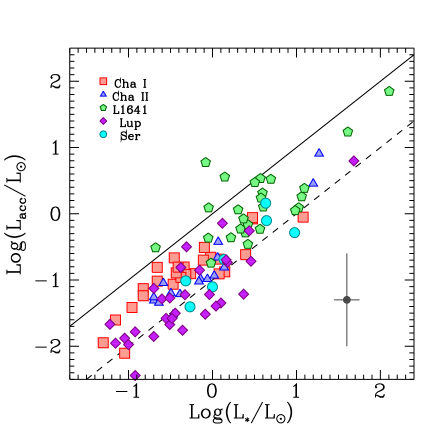
Figure 4: Accretion luminosity as a function of the stellar luminosity for the whole POISSON sample. The various symbols refer to the five different cloud samples (see legend). The solid and dashed lines show the locus of $L_{\mathrm{acc}}$=$L_{\mathrm{*}}$  and $L_{\mathrm{acc}}$=0.1$L_{\mathrm{*}}$.

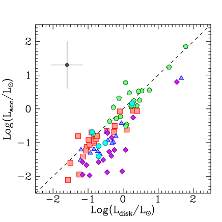
Figure 5: Accretion luminosity plotted as a function of the disk luminosity for the POISSON sources. Symbols are the same as in Fig. 4. The dashed line shows the locus of equal $L_{\mathrm{acc}}$ and $L_{\mathrm{disk}}$.

However, the plot also shows that several sources, especially in the Lupus sample, display an accretion luminosity that is significantly lower (about one order of magnitude) than the observed disk luminosity. Therefore in these stars the bulk of the excess luminosity does not come from the accretion process, which suggests intrinsic emission from massive disks.

Alternatively, a possible interpretation is that these might be edge-on objects in which the central star and innermost accretion region are heavily extincted (the so-called sub-luminous sources, see e.g. discussion in Alcalà et al. 2014), causing an underestimation of both $L_{\mathrm{acc}}$ and $L_{\mathrm{*}}$ that is difficult to predict.

4.3 Mass accretion rates

The mass accretion rates of the whole sample range from $10^{-7}$ to $10^{-9}$ M_⊙ yr^-1, with a few objects in L1641 showing higher $\dot{M}_{acc}$ values of about $10^{-6}$ M_⊙ yr^-1. Based on the same considerations as in Sect. 3, we can assume a typical uncertainty on these $\dot{M}_{acc}$ values of about 0.8 dex. In Fig. 6 we analyse the correlation of the mass accretion rate with both the mass and age of the POISSON sample (left and right panels). Despite the huge scatter, a rough trend of $\dot{M}_{acc}$ increasing with $M_{\mathrm{*}}$ can be seen in the plot on the left. Indeed, from computing the Spearman rank correlation coefficient ($r$), we find $r=0.42$ with a probability of obtaining this from randomly distributed data $p\sim 10^{-5}$.

A power-law relationship $\dot{M}_{acc}$ $\propto M_{*}^{\beta}$ with $\beta$ around 2 has been observed in several star-forming regions in recent years, for samples with masses and ages very similar to those explored by POISSON, see for instance $\beta$=2.1 (Muzerolle et al. 2005), $\beta$=1.8 (Natta et al. 2006), $\beta$=1.9 (Herczeg & Hillenbrand 2008), $\beta$=1.8 (Alcalá et al. 2014). The function $\dot{M}_{acc}$ $\sim M_{*}^{2}$ is marked with a dotted line in the left panel of Fig. 6 for reference.

In paper I, we found an analogous correlation ($\propto$$M_{\mathrm{*}}$^1.95) from limiting our analysis only to Cha I objects. Here we considered all POISSON sources to improve the statistics, but found that the data points are so scattered (with a dispersion even greater than two orders of magnitude) that it is practically impossible to achieve a reliable fit on the whole dataset.

A trend of accretion rate decreasing with time is visible for the $\dot{M}_{acc}$ versus age plot. The five sub-samples display different median values of $\dot{M}_{acc}$ (disregarding upper limits), from $\sim 1\times 10^{-7}$ M_⊙ yr^-1in L1641 down to $\sim 6\times 10^{-9}$ M_⊙ yr^-1in Lupus. This decreasing median rate reflects an increasing median age of the five investigated samples, which spans from $\sim 8\times 10^{5}$ yr for L1641 to $\sim$3 Myr for Lupus, in agreement with the expected decay of $\dot{M}_{acc}$ as sources evolve.

The observed evolution trend can be compared with the $\dot{M}_{acc}$ temporal variation predicted by Hartmann et al. (1998) for viscous disk models (see for example Muzerolle et al. 2000, Sicilia-Aguilar et al. 2010, and paper II). A typical fiducial model considered by Hartmann et al. (1998) assumes a 0.5 M_⊙ star, constant viscosity $\alpha=10^{-2}$, and a viscosity exponent $\gamma=1$. $\dot{M}_{acc}$ evolution predictions based on this fiducial model are shown in Fig. 6 using two dashed curves, which refer to two different initial disk masses of 0.1 (lower) and 0.2 (upper) M_⊙.

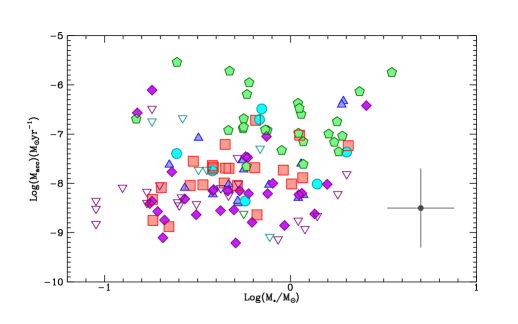
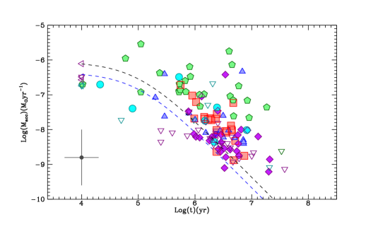
Figure 6: Mass accretion rates of the whole POISSON sample plotted as a function of the stellar mass (left) and age of the targets (right). Upper limits on $\dot{M}_{acc}$ are indicated by downward triangles. The typical error bar of a single point is also shown. The dashed lines in the right graph show the expected $\dot{M}_{acc}$ evolution for a fiducial model of a viscous disk (Hartmann et al. 1998) (see text for more details) around a 0.5M_⊙ star with initial disk masses equal to 0.1M_⊙ (lower line) and 0.2M_⊙ (upper line). Sample symbols are the same as in Fig. 4.

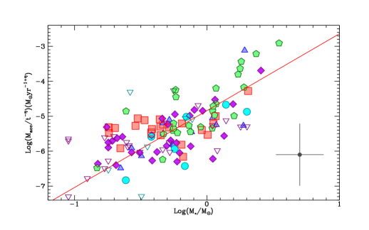
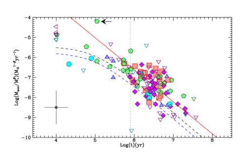
Figure 7: Same as in Fig. 6, but for normalised data: $\dot{M}_{acc}$ normalised by the time factor provided by Hartmann et al. (1998) $\dot{M}_{acc}$ evolution models ($\sim t^{-\eta}$, see text) vs $M_{\mathrm{*}}$ (right) and $\dot{M}_{acc}$ normalised by $M_{\mathrm{*}}$^β vs age (right; $\dot{M}_{acc}$ evolution curves by Hartmann et al. are also normalised). The best-fit relationships we obtain are indicated with a solid red line and correspond to power-law indexes $\beta=2.2$ (left) and $\eta=1.6$ (right). The vertical dotted line in the right graph shows the lower limit on age that we considered for the fit of the power -law decrement. The position of the outbursting source V2775 Ori (paper II, Caratti o Garatti et al. 2011) is marked by an arrow in the temporal evolution plot.

In these models the $\dot{M}_{acc}$ evolution is typically slower at early time, then it asymptotically tends to a power-law decay of the type $\dot{M}_{acc}$ $\sim t^{-\eta}$, when the elapsed time is much longer than the initial characteristic viscous time of the disk. For the fiducial models reported, the asymptotic relationship is $\dot{M}_{acc}$ $\sim t^{-1.5}$, which is approximately reached when Log $t>5.9$.We also note that the initial disk mass ($M_{D}$) substantially sets the initial value of the accretion rate. Accretion luminosities in the range 0.1 $L_{\mathrm{*}}$$<$$L_{\mathrm{acc}}$$<$ $L_{\mathrm{*}}$, such as those observed by POISSON, are compatible with sources having a mass of 0.5-1.0 M_⊙ and a disk-to-star mass ratio of 0.2-0.1 (Tilling et al. 2008), so that the 0.1-0.2 M_⊙ disk masses considered in the plot are in the range of the expected upper limit values of $M_{D}$ for a solar-type star. Even if the decay trend of accretion rates is very similar to the expected evolution for viscous disks, most of the measured $\dot{M}_{acc}$ values appear to be higher than those predicted by the models. Moreover, the data point spread at similar age is very large, so that we find several sources that show accretion rates up to two orders of magnitude greater than those of the fiducial viscous models considered, in particular among L1641 objects.

Before further investigating this discrepancy between models and observed points (Sect. 4.5), we applied a procedure similar to the one we used in paper II for L1641 objects and normalised $\dot{M}_{acc}$ by $M^{\beta}$ (when plotting $\dot{M}_{acc}$ versus time) and $t^{-\eta}$ (when plotting $\dot{M}_{acc}$ versus $M_{\mathrm{*}}$), which we can assume as the power-law index relationships that describe the dependence of $\dot{M}_{acc}$ on $M_{\mathrm{*}}$ and age. In fact, since the accretion rate depends on both $M_{\mathrm{*}}$ (explicitly, see Eq. 3) and age (implicitly, because the accretion rate is expected to vary with time), this operation allows us to remove from the plotted accretion rate values the implicit dependence on one of the two parameters, so that in the resulting plot we are able to better visualise the actual $\dot{M}_{acc}$ dependence on the other parameter alone. In particular, normalising by the age and mass helps to reduce the impact on our analysis that arises from the slightly different mass and age distributions of the samples.

Because we do not know a priori the values of $\eta$ and $\beta$, we used a procedure in which we simultaneously fit the two normalised datasets to derive the best-fit values of both power-law indexes. Using an ordinary least-square bisector linear regression and excluding upper limits, we obtain the best-fit relations marked as solid red lines in Fig. 7.

For the dependence on the stellar mass alone we obtain $\dot{M}_{acc}$ $\sim$ $M_{\mathrm{*}}$^2.2±0.3 with a significantly stronger higher coefficient ($r=0.62$, $p<10^{-10}$) than in the non-normalised plot. The power-law index is therefore consistent with the slope $\beta\sim 2$ observed in other star-forming regions. Ercolano et al. (2014) have recently considered more than 3000 $\dot{M}_{acc}$ determinations from the literature, obtained in various star-forming regions, to derive the power-law index of the $\dot{M}_{acc}$–$M_{\mathrm{*}}$ relationship. The authors infer a value of $\beta$ in the range 1.6–1.9, but limited to stars with $M_{\mathrm{*}}$$<$ 1M_⊙. Interestingly, if we restrict our fit to stars with masses below 1M_⊙ in our sample, we obtain a power-law index of 1.7, fully consistent with the result found by Ercolano et al.

For the rate evolution at long times $\dot{M}_{acc}$ decays as $t^{-1.6\pm 0.2}$. We point out that in this case we limited the regression only to the region of the plot where the evolution is described by a power-law function (i.e. ages greater $t\gtrsim$ 1 Myr). Also here we obtain a tighter (anti)correlation for normalised data, that is, $r=-0.42$ with $p\sim 0.0001$ against $r=-0.28$ with $p\sim 0.01$ for the previous plot. We note that three sources in Lupus and one in L1641 show ages older than 10 Myr, which appears to be strangely high for these regions. As this might stem from an incorrect determination of the stellar luminosity (e.g. sources viewed edge-on), we decided to perform the fit also by excluding these objects. We still obtain an accretion decay that behaves as $t^{-1.6\pm 0.2}$, although with a weaker correlation ($r=-0.34$ with $p\sim 0.003$). The value of the power-law index $\eta$ is very similar to that of the fiducial model considered ($\eta$=1.5), and it falls within the interval 1.5-2.8 originally suggested by Hartmann et al. (1998). Thanks to the fairly large statistics available, we are confident that the observed general trend is real, even if uncertainties on age and accretion luminosities of the single points are relatively large. Nonetheless, most of the $\dot{M}_{acc}$ values still appear to be higher than those predicted for the viscous models: possible reasons for this finding are discussed in the following sections.

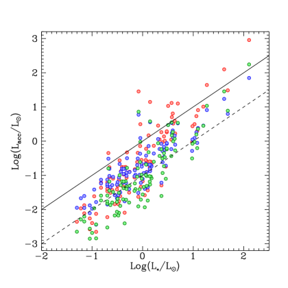
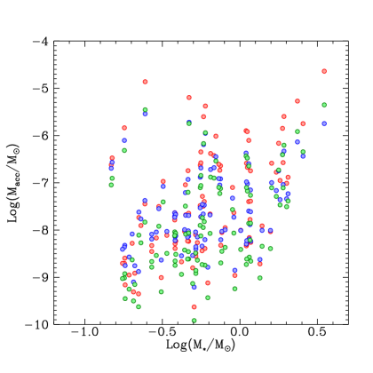
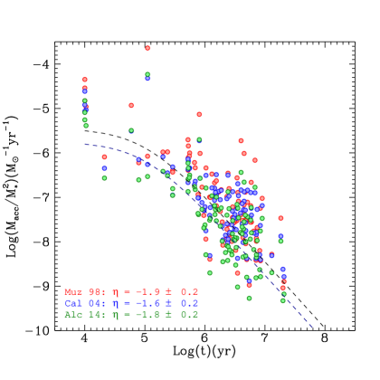
Figure 8: Results obtained by considering $L_{\mathrm{acc}}$ values from with three different empirical relationships for Br$\gamma$: Alcalá et al. (2014) (green), Muzerolle et al. (1998) (red), and Calvet et al. (2004) (blue). Displayed plots are $L_{\mathrm{acc}}$ versus $L_{\mathrm{*}}$ (top), $\dot{M}_{acc}$ versus $M_{\mathrm{*}}$ (centre), and $\dot{M}_{acc}$ normalised to $M_{\mathrm{*}}$² versus age (bottom). In the last plot we report the curves of the viscous disk model of Hartmann et al. (1998) shown in Figs. 6 and 7; the best-fit power-law indexes obtained from the different distributions for sources with Log $t>5.9$ (see text for details) are also indicated.

4.4 Results from different line-$L_{\mathrm{acc}}$ relationships

In Sect. 4.3 we found that $\dot{M}_{acc}$ values obtained from Eq. 1 appear to be overestimated in general with respect to the predictions of viscous disk models. Therefore, we investigated the possible systematic effects caused by the empirical relationships adopted to convert H i line luminosities into $L_{\mathrm{acc}}$. We considered two additional relationships, the classical formula provided by Muzerolle et al. (1998) and the recent calibration by Alcalá et al. (2014), based on VLT/X-Shooter observations of a sample of Lupus objects:

$$\mathrm{Log}\;L_{acc}/L_{\odot}=1.26\cdot\mathrm{Log}\;L_{\mathrm{Br\gamma}}/L_{\odot}+4.43\leavevmode\nobreak\ ,$$ (5)

$$\mathrm{Log}\;L_{acc}/L_{\odot}=1.16\cdot\mathrm{Log}\;L_{\mathrm{Br\gamma}}/L_{\odot}+3.60\leavevmode\nobreak\ .$$ (6)

The three relationships yield accretion luminosities that may significantly differ from each other depending on the line luminosity range involved. This is evident in the upper panel of Fig. 8 where we show the $L_{\mathrm{acc}}$ vs $L_{\mathrm{*}}$ plot we obtain with the three relationships. The different $L_{\mathrm{acc}}$ vs $L_{\mathrm{*}}$ trends we observe obviously reflect the different parameters of the laws, and the relationships of Muzerolle and Alcalá provide lower accretion luminosities for lower luminosity stars. In particular, the differences with values reported by Alcalá are about 0.7 dex for the less luminous stars of our sample ($\sim$0.4 dex for a solar-type star).

Of course, the same differences are found for the mass accretion rates, which are directly proportional to $L_{\mathrm{acc}}$. The $\dot{M}_{acc}$ vs $M_{\mathrm{*}}$ plot is shown in the central panel of Fig. 8. In this case, we note that although the single $\dot{M}_{acc}$ values may significantly differ in the three cases, the general distribution of the points in the plot does not change substantially.

The $\dot{M}_{acc}$ evolution plots displayed in the lower panels of Fig. 8 show that the generally lower $\dot{M}_{acc}$ values obtained from the Alcalà (and Muzerolle) relationship agree better with the rates expected for a viscous disk evolution, with more points falling along or below the viscous disk curves of the reference fiducial models we considered in Sect. 4.3. However, even though the general agreement of the measurements with the models is improved, we still observe a large number of source points located above the curves. This means that the systematic effect caused by the adopted relationship alone cannot explain these higher-than-expected $\dot{M}_{acc}$ values, so we need to invoke other causes, which we discuss in Sect. 4.5.

Additionally, although the use of a different line-$L_{\mathrm{acc}}$ relation leads to fairly large variations of the single accretion rate estimates, this does not seem to heavily affect the general trend of the $\dot{M}_{acc}$ evolution. Indeed, we obtain that the power-law index describing the $\dot{M}_{acc}$ time evolution is very similar in the three cases, with best-fit $\eta$ values of 1.6$\pm$0.2 (Calvet), 1.9$\pm$0.2 (Muzerolle), and 1.8$\pm$0.2 (Alcalá), which are substantially consistent with each other considering uncertainties (see Fig 8).

4.5 Accretion rate evolution

In the previous sections we found that the variation of $\dot{M}_{acc}$ with time roughly follows the trend expected from viscous evolution, although two open problems needed to be further investigated: i) the evidence of a large spread of $\dot{M}_{acc}$ values for objects with similar age, even after considering ”normalised” accretion rates, and ii) the presence of many measured accretion rates significantly higher than those expected for a viscous disk evolution (Hartmann et al. 1998), which we obtain also allowing for systematic effects due to the employed empirical H i-$L_{\mathrm{acc}}$ relation (Sect. 4.4).

The time evolution of the accretion rate has recently been studied in several papers (e.g. Muzerolle et al. 2000; Sicilia-Aguilar et al. 2006, 2010). In particular, Sicilia-Aguilar et al. (2010) analysed the relationship between accretion rates and ages collected for sources from various star-forming regions (see their Fig. 2). These authors found a good general agreement between $\dot{M}_{acc}$ measurements and the evolution trend predicted by viscous disk models, although in their analysis the measurements are also characterised by a large spread around the model curves and by numerous data points that are higher than those predicted for fairly massive accretion disks.

Despite the uncertainties, the large $\dot{M}_{acc}$ spread we observe is most likely a real effect. Indeed, within the framework of viscous accretion, a high dispersion of $\dot{M}_{acc}$ is automatically obtained by considering a range of initial disk masses because the predicted $\dot{M}_{acc}$ is directly proportional to $M_{D}$ (Hartmann et al. 1998). This scenario can partly explain the dispersion observed, but it can be reasonably invoked only for points that lie around or below the curves relative to $M_{D}$ of 0.1 and 0.2 M_⊙(see Fig. 7), which substantially represent the upper limit for disk masses around solar-type stars.

Another possible way to explain the scatter of $\dot{M}_{acc}$ points is to assume that the initial conditions and/or the physical processes are not the same in the various disks. Strong observational evidence supporting the presence of very different viscosity laws in the disks was recently provided by Isella et al. (2009), who revealed a wide variety of viscosity parameters for several solar-type objects. For instance, by considering a different viscosity parameter $\alpha$ in the disk models, we obtain $\dot{M}_{acc}$ evolution curves that may significantly differ from the fiducial model curves considered in Sect. 4.3 (see examples in Hartmann et al. 1998).

Varying accretion through recurrent bursts may also be at the origin of the strong discrepancies of $\dot{M}_{acc}$ with respect to the expected average level of accretion at a certain age. Powerful accretion bursts are predicted by recent accretion theoretical models (e.g. Vorobyov & Basu 2006). Although we have evidence that most sources of the sample are not in an outbursting stage, variable accretion may effectively contribute to the observed scatter of $\dot{M}_{acc}$ data points. In our sample we find clear evidence for this effect in [MJS2008] 146 and especially in the extreme case of V2775 Ori, which shows an $\dot{M}_{acc}$ about two orders of magnitude greater than predicted in the normalised plot of Fig. 7.

While for the accretion rate decay at long times we obtain $\dot{M}_{acc}$ $\sim t^{-1.6}$, which is very similar to the $\sim t^{-1.5}$ trend of the fiducial viscous disk model, Sicilia-Aguilar et al. (2010) found a relationship $\dot{M}_{acc}$ $\sim t^{-1.2}$, suggesting a somewhat slower decrease of the mass accretion rate. Noticeably, this is the same value of the power-law index as we inferred for L1641 objects alone in paper II, although we point out that in our previous work we considered also younger sources in the fit, with ages between 10⁵ and 10⁶ yr, in which the asymptotic $\dot{M}_{acc}$ evolution trend might not be reached yet. Our analysis is limited because the bulk of the POISSON data points is in the (restricted) age range of 1-10 Myr and typically presents an $\dot{M}_{acc}$ dispersion of about $\sim$2 dex. The sample studied by Sicilia-Aguilar et al. (2010) has the advantage of presenting a mean age older than the regions studied here, which allows on the one hand to better constrain the $\dot{M}_{acc}$ decay for t $\gtrsim$ 10 Myr, and on the other hand to somewhat minimise the age spread uncertainties for individual objects.

On the other side of the plot, the very low number of very young sources allows us to derive only a marginal evidence of the expected slower evolution of the mass accretion rate at early times ($t\lesssim$ 1Myr) in Fig. 7. The moment of the onset of the asymptotic decline of $\dot{M}_{acc}$ depends on the parameters of the disk (such as viscosity and dimensions), therefore a better sampling of this region would possibly provide information on these aspects.

Another effect that may alter the evolution of the mass accretion rate is the presence of additional processes that might be adding to disk dissipation, such as photo-evaporation (e.g. Gorti et al. 2009; Owen et al. 2012). Indeed, a very efficient photo-evaporation would dissipate the disk in a short time because a rapid cut-off of $\dot{M}_{acc}$ (with a time-scale of about 10% of the disk lifetime) is expected when the accretion rate drops below the photo-evaporation rate (e.g. Ercolano et al. 2014). Sicilia-Aguilar et al. (2010) invoked this mechanism to explain the presence of many objects without significant accretion ($\dot{M}_{acc}$$\lesssim 10^{-11}$ M_⊙ yr^-1) in a wide range of ages ($t\gtrsim 1$Myr). In our sample we observe only a few of these upper limits in Fig. 7, mostly among evolved Lupus sources with ages $>$5Myr. This finding may suggest that the photo-evaporation is not the dominant process in many of the disks observed by POISSON, although its presence can accelerate the decay of $\dot{M}_{acc}$ in some objects and thus produce the large spread of the accretion rates that we observe. Indeed, the models (e.g. Owen et al. 2011, 2012) show that the quick drop of $\dot{M}_{acc}$ at times $t\gtrsim 1$Myr induced by the X-ray photo-evaporation may easily produce a large spread of the accretion rates starting from the expected viscous decay, depending on the X-ray flux of the sources (see for instance Fig. 7 of Owen et al., 2011) and on the initial disk properties. Moreover, this would provide a somewhat steeper general decline of $\dot{M}_{acc}$ with respect to viscous evolution when fitting the whole sample, which we marginally detect. In a scenario where photo-evaporation regulates disk dissipation for most objects, the lack of detection of non-accreting sources might be related to the the selected sample being only composed of relatively bright objects, which might partly explain why our results appear generally biased towards high average values of the mass accretion rate.

5 Conclusions

We have presented the results of POISSON near-infrared spectroscopic observations of two samples of low-mass (0.1-2.0M_⊙) young stellar objects in Lupus (52 sources) and Serpens (17 sources). We have derived the accretion luminosities $L_{\mathrm{acc}}$ and mass accretion rates $\dot{M}_{acc}$ of the targets using the H i Br$\gamma$ line (Pa$\beta$ in a few cases) and the relevant empirical relationship connecting the flux of the line to $L_{\mathrm{acc}}$.

The new results from the Lupus and Serpens samples were then added to previous results from our POISSON papers I and II (on Cha I,Cha II, and L1641 clouds) to build a large catalogue of the whole POISSON sample, composed of 143 objects with masses in the range 0.1-3.5 M_⊙ and ages between $10^{4}$ and few $10^{7}$ years. For all these sources we obtained $\dot{M}_{acc}$ estimates computed in a homogeneous and consistent fashion and analysed in particular the $\dot{M}_{acc}$ correlation with stellar mass ($M_{\mathrm{*}}$) and its evolution through time.

We observe a correlation $\dot{M}_{acc}$$\sim$$M_{\mathrm{*}}$^2.2 between mass accretion rate and stellar mass, similar to the correlation observed in several star-forming regions. We also find that the temporal variation of $\dot{M}_{acc}$ is roughly consistent with the expected evolution of the accretion rate in viscous disks, with an asymptotic decay proportional to $t^{-1.6}$. However, sources with similar age are characterised by $\dot{M}_{acc}$ values that display a large scatter and are generally higher than the predictions of viscous models. Although part of these aspects may be related to systematics due to employed empirical relationship and to the relatively big uncertainties on the single measurements, the large statistics available make us confident that the general distribution and decay trend of the $\dot{M}_{acc}$ points are real. In particular, the observed $\dot{M}_{acc}$ scatter might be indicative of a large variation in the initial mass of the disks, of fairly different viscous laws among disks, of varying accretion regimes, and of other mechanisms that add to the dissipation of the disks, such as photo-evaporation.

Appendix A: near-IR photometry.

Measured $JHK$ magnitudes of the sources are reported in Tables 6 and 7 together with 2MASS photometry, which is given for comparison. Small photometric variations (over time-scales of months/years) of about a few tenths of magnitude in the near-IR are typical of young objects (e.g. Alves de Oliveira & Casali 2008) and are generally attributed to varying accretion activity or extinction variations (see e.g. Carpenter et al. 2001).

In our samples most of the sources display this type of fluctuation, with a mean magnitude variation (in absolute value) of about 0.2, 0.1, and 0.1 mag ($JHK$-bands, respectively) in Lupus and 0.2, 0.2, and 0.4 mag in Serpens.

However, we were also able to identify a few objects that underwent significant brightness variations (of about 1 mag or greater in at least one of the bands): Sz98, [MJS2008] 133, and [MJS2008] 146 in Lupus and [WMW2007]70 and [WMW2007]4 in Serpens. In particular, [MJS2008] 133 appears much dimmer in POISSON data than in 2MASS observations and displays photometric variations of $\Delta J=-1.5$, $\Delta H=-1.9$ $\Delta K=-2.0$ mag (Antoniucci et al. 2013b). These pronounced photometric fluctuations might indicate an EXor- (e.g. Lorenzetti et al. 2011) or UXor-type (e.g. Shenavrin et al. 2012) variability for these objects.

Table 6: Near-infrared photometry of the Lupus targets derived from POISSON data, compared with 2MASS magnitudes. Typical uncertainty on the provided values is 0.05 mag for the $H$ band and 0.1 mag for $J$ and $K$ bands (see text for details).

ID	$J$	$H$	$K$	$J$	$H$	$K$
	2MASS			POISSON
01	9.19	8.41	7.98	8.9	8.32	8.1
02	10.89	9.88	9.29	10.2	9.54	9.2
03	12.2	10.64	9.71	11.9	10.53	9.8
04	7.57	6.86	6.48	7.2	6.81	6.5
05	11.18	10.16	9.41	10.8	10.02	9.42
06	11.64	10.95	10.48	11.8	11.15	10.4
07	10.07	9.18	8.63	10.2	9.4	9.0
08	10.57	9.77	9.33	10.7	9.93	9.5 5
09	10.74	9.53	8.83	10.8	9.59	8.7 6
10	8.69	7.7	7.1	8.3	7.41	6.8
11	8.78	8.09	7.74	8.6	7.87	7.5
12	8.73	7.82	7.14	8.6	7.74	7.0
13	10.93	10.2	9.85	11.0	10.27	10.0
14	8.55	7.69	6.98	8.2	7.59	7.0
15	8.16	7.06	6.12	7.3	6.33	5.8
16	8.71	7.53	6.9	8.8	7.92	7.3
17	9.46	8.68	8.35	8.9	8.38	8.2
18	9.73	8.96	8.5	9.6	8.98	8.8
19	12.11	10.55	9.53	11.8	10.43	9.5
20	9.92	9.12	8.56	9.8	9.1	8.6
21a	…	…	…	11.3	10.7	10.4
22	11.51	10.65	10.11	11.4	10.68	10.2
23	10.35	9.32	8.72	10.5	9.48	8.9
24	11.01	10.28	10.01	11.0	10.27	10.1
25	10.03	8.53	7.67	9.7	8.33	7.6
26	10.13	9.35	8.96	10.3	9.46	9.0
27	11.24	10.55	10.22	11.2	10.55	10.3
28	9.53	8.65	8.01	10.7	9.47	8.6
29	11.93	11.21	10.75	11.8	11.22	10.9
30	10.98	10.35	9.91	10.8	10.29	9.9
31	11.38	10.62	10.23	11.1	10.59	10.4
32	8.97	8.39	8.22	9.0	8.38	8.2
33	11.67	11	10.65	11.5	10.98	10.7
34b	5.91	5.22	4.39	6.0	5.22b	4.3
35	11.65	10.66	10.15	11.5	10.53	10.1
36	11.25	10.62	10.31	11.1	10.58	10.4
37	11.4	10.82	10.5	11.3	10.82	10.7
38	11.45	10.17	9.55	11.5	10.27	9.8
39	10.97	10.22	9.75	10.8	10.17	9.9
40	11.33	10.28	9.8	11.3	10.28	9.9
41	10.62	9.8	9.54	10.5	9.82	9.6
42	11	10.29	9.96	11.0	10.32	9.9
43	12.47	11.72	11.26	12.5	11.64	11.1
44	10.41	9.7	9.32	10.3	9.64	9.3
45	10.68	9.85	9.43	10.5	9.84	9.7
46	10.45	9.35	8.68	10.4	9.38	8.8
47	12.66	12.09	11.76	12.8	12.11	11.8
48	13.28	12.65	12.32	13.4	12.72	12.3
49	11.09	10.21	9.78	11.0	10.18	9.8
50	11.84	10.28	9.41	13.3	12.19	11.4
51	10.63	9.6	8.96	10.5	9.5	8.9
52	10.54	9.77	9.54	10.5	9.82	9.5

Notes.
^a this secondary component was not spatially resolved in 2MASS.
^b 2MASS $H$ magnitude was used to calibrate the RG spectrum of HR5999.

Table 7: Near-infrared photometry of the Serpens targets derived from POISSON data, compared with 2MASS magnitudes. Typical uncertainty on the provided values is 0.05 mag for the $H$ band and 0.1 mag for $J$ and $K$ bands (see text for details).

ID	$J$	$H$	$K$	$J$	$H$	$K$
	2MASS			POISSON
01	11.6	10.39	9.64	…	10.44	9.5
02	13.9	12.45	11.6	…	13.12	12.2
03	16.89	15.66	12.67	…	15.66	13.4
04	12.61	11.24	10.41	12.7	11.38	10.6
05	15.34	12.47	10.65	…	12.86	11.3
06	15.01	12.81	11.52	…	12.65	11.6
07	15.17	12.47	11.09	…	12.46	11.2
08	12.22	9.24	7.05	12.7	9.57	7.5
09	16.21	12.79	10.81	…	12.79	11.1
10	18.17	15.82	12.97	…	15.63	14.5
11	17.2	14.41	11.66	…	14.36	11.5
12	15.75	12.46	10.52	…	12.32	10.1
13	13.07	11.19	9.86	…	10.91	9.8
14	15.19	14.03	11.84	…	14.56	12.8
15	15.2	11.92	9.92	…	12.29	10.3
16	12.28	11.05	10.38	12.3	10.96	10.4
17	12.25	10.84	10.07	12.7	11.19	10.5

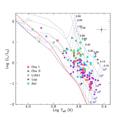
Figure 9: HR diagram for the sources of the five star-forming clouds analysed in POISSON (see legend). Superposed evolutionary tracks for labelled stellar masses in M_⊙ (grey lines), isochrones for labelled time in years (blue dashed lines), ZAMS (solid red line), and early main sequence (dashed red lines) are taken from the models of Siess et al. (2000). The point with error bars shows the mean uncertainty on the position of the single sources.

Appendix B: determination of $L_{\mathrm{disk}}$, $M_{\mathrm{*}}$, and age.

Source disk luminosities employed in Sect. 4.2 were not available in the literature for Cha (paper I) and L1641 objects (paper II), therefore these were obtained using the estimates of the bolometric and stellar luminosities: $L_{\mathrm{disk}}$=$L_{\mathrm{bol}}$–$L_{\mathrm{*}}$. However, since the $L_{\mathrm{*}}$ values given in paper II for L1641 objects had been obtained as $L_{\mathrm{bol}}$–$L_{\mathrm{acc}}$, to determine $L_{\mathrm{disk}}$ entirely independently of $L_{\mathrm{acc}}$ (like for other sub-samples), we have re-derived $L_{\mathrm{*}}$ from the spectral type and $I$ magnitude of the objects ($J$ magnitude when $I$ was not available) by integrating a NEXTGEN stellar spectrum (Hauschildt et al. 1999) of the same spectral type as the object normalised to the observed $I$ ($J$) band flux. The new $L_{\mathrm{*}}$ values thus obtained for L1641 are listed in Table 8.

As mentioned in Sect.4.1, to minimise systematic biases we decided to (re-)determine $M_{\mathrm{*}}$ and age of all POISSON sources on the basis of the same pre-main sequence evolutionary models. For this task we considered the models by Siess et al. (2000, 1999), assuming a metallicity Z=0.2 and no overshooting. The relative evolutionary tracks and isochrones are displayed in the HR diagram in Fig. 9. Mass and age of the single objects were computed by interpolating (where possible) over the model grid. For sources located outside the area covered by the model grid only upper limits to the parameters are provided.

The main stellar parameters ($L_{\mathrm{*}}$, $T_{\mathrm{eff}}$, Spectral Type, $M_{\mathrm{*}}$, age) of all POISSON objects are listed (per region) in Tables 8 and  9, together with the determined mass accretion rate.

Table 8: Main parameters of POISSON sources in Cha I, Cha II, and L1641, investigated in papers I and II. Masses and ages (re)determined from HR diagram position using the models of Siess et al. (2000), in conjunction with $\dot{M}_{acc}$values derived from Br$\gamma$.

ID	Name	$L_{\mathrm{*}}$(L⊙)	$T_{\mathrm{eff}}$(K)	ST	$M_{\mathrm{*}}$(M⊙)	age(yr)	$\dot{M}_{acc}$(M⊙ yr-1)
Chamaeleon I
01	T11	1.20	4205	K6	0.91	1.9E+06	1.9E-08
02	CHSM1715	0.05	3234	M5	0.18	7.4E+06	1.8E-09
03	T14	0.95	4350	K5	1.16	4.3E+06	1.3E-08
04	ISO52	0.09	3270	M4	0.22	4.8E+06	1.3E-09
05	Hn5	0.11	3198	M5	0.20	3.5E+06	8.2E-09
06	ISO92	…	…	…	…	…	…
07	ISO97	…	…	…	…	…	…
08	T26	12.0	5860	G2	2.04	4.7E+06	5.8E-08
09	B35	…	…	…	…	…	…
10	CHXR30B	0.22	3669	M1	0.44	4.4E+06	1.0E-08
11	T30	0.15	3488	M2	0.34	4.5E+06	9.3E-09
12	CHXR30A	1.40	3955	K7	0.64	9.7E+05	2.9E-08
13	T31	3.00	3955	K7	0.65	5.6E+05	1.9E-07
14	Cha IRN	…	…	…	…	…	…
15	C9-3	…	…	…	…	…	…
16	T38	0.34	3778	M0	0.52	3.4E+06	9.1E-09
17	CHXR79	0.55	3669	M1	0.45	1.5E+06	2.0E-08
18	C1-6	0.80	3669	M1	0.45	1.0E+06	6.2E-08
19	C1-25	…	…	…	…	…	…
20	Hn10-e	0.15	3379	M3	0.29	3.6E+06	9.1E-09
21	B43	0.22	3379	M3	0.30	2.4E+06	2.8E-08
22	T42	3.00	4350	K5	1.12	8.9E+05	9.5E-08
23	T43	0.48	3560	M2	0.38	1.4e+06	2.3E-08
24	C1-2	…	…	…	…	…	…
25	Hn11	0.66	3955	K7	0.66	2.4E+06	2.3E-09a
26	ISO237	1.20	4278	K5	1.01	2.4E+06	9.7E-09
27	T47	0.42	3560	M2	0.38	1.7E+06	2.0E-08
28	ISO256	0.07	3198	M5	0.18	5.1E+06	4.7E-09
29	T49	0.37	3560	M2	0.38	1.9E+06	2.1E-08
30	T53	0.39	3705	M1	0.47	2.3E+06	2.0E-08
Chamaeleon II
01	DKCha	18.62	7200	F0	1.92	6.8E+06	4.7E-07
02	IRAS12535-7623	1.38	3850	M0	0.55	7.9E+05	3.0E-08
03	ISO ChaII 28	15.85	4500	K4	1.88	2.9E+05	4.0E-07
04	Sz49	0.20	3777	M0	0.52	7.2E+06	4.0E-09
05	Sz48SW	0.26	3705	M1	0.46	3.9E+06	9.6E-09
06	Sz50	1.15	3415	M3	0.32	2.0E+05	8.4E-08
07	CMCha	0.72	4060	K7	0.76	2.8E+06	9.4E-09
08	IRAS13005-7633	0.23	3560	M2	0.38	3.2E+06	6.0E-09
09	Hn23	0.87	4350	K5	1.17	5.0E+06	5.8E-09
10	Hn24	1.05	3850	M0	0.56	1.0E+06	1.9E-08
11	Sz53	0.32	3705	M1	0.47	3.0E+06	7.4E-09
12	Sz56	0.34	3270	M4	0.27	1.55E+06	8.1E-09
13	Sz57	0.41	3125	M5	0.22	2.9E+05	2.4E-08
14	Sz58	0.69	4350	K5	1.10	7.1E+06	5.0E-09
15	Sz61	1.17	4350	K5	1.14	3.1E+06	2.5E-08
16	IRASF13052-7653NW	0.20	3777	M0	0.52	7.2E+06	4.4E-09
17	IRASF13052-7653N	0.34	3632	M1	0.42	2.3E+06	$<$8.0E-09
L1641
01	[CHS2001]13811	0.89	4350	K5	1.17	4.8E+06	2.4E-08
02	[CTF93]50	11.55	4200	K6	1.10	2.4E+05	4.2E-07
03	[CTF93]47	40.93	9230	A1	2.35	4.5E+06	7.3E-07
04	[CTF93]32	2.46	3850	M0	0.55	5.2E+05	1.3E-07
05	[CTF93]72	2.02	4350	K5	1.10	1.4E+06	1.0E-07
06	[CTF93]83	3.68	4060	K7	0.75	5.2E+05	1.2E-07
07	[CTF93]62	10.63	8200	A6	1.81	1.8E+07	4.4E-08
08	[CTF93]79	127.29	13000	B7	3.50	4.0E+06	1.8E-06
09	[CTF93]99	4.02	4590	K4	1.60	1.2E+06	1.0E-07
10	[CTF93]87	2.16	3850	M0	0.56	5.5E+05	1.4E-07
11	[CTF93]104	3.73	5250	K0	1.78	5.9E+06	1.8E-07
12	Meag31	0.96	2800	M7	0.15	1.0E+04	2.0E-07
13	[CTF93]146-2	2.64	3705	M1	0.46	1.1E+05	1.2E-07
14	[CTF93]146-1	1.40	3890	K7	0.58	8.1E+05	6.4E-07
15	[CTF93]211	2.64	4060	K7	0.73	6.7E+05	1.2E-07
16	[CTF93]187	9.67	6280	F7	1.72	8.4E+06	6.9E-08
17	[CTF93]168	3.94b	4350	K5	1.14	6.7E+05	2.5E-07
18	[CTF93]191	3.78	5080	K1	1.90	4.2E+06	9.2E-08
19	[CTF93]246A	0.21b	3850	M0	0.58	9.0E+06	2.2E-08
20	[CTF93]186	3.19b	4350	K5	1.11	8.3E+05	3.3E-07
21	[CTF93]246B	2.34	3850	M0.	0.56	5.3E+05	2.1E-07
22	[CTF93]237-2	0.09	3850	M0	0.56	3.3E+07	$<$2.4E-09
23	[CTF93]237-1	4.96	3850	M0	0.60	5.9E+04	1.1E-06
24	[CTF93]216-1	12.44b	3560	M2	0.47	$<$1.0E+04	1.9E-06
25	[CTF93]216-2	0.83b	3200	M5	0.24	1.1E+05	2.9E-06
26	[CTF93]245B-2	0.90	4350	K5	1.17	4.7E+06	7.0E-08
27	[CTF93]245B-1	1.66	4200	K6	0.89	1.2E+06	4.7E-08

Notes. ^a $\dot{M}_{acc}$ computed from Pa$\beta$. ^b $I$ magnitude not available for ST spectrum normalisation, $J$ magnitude used (see appendix).

Table 9: Same as Table 8 for the POISSON sources of Ser and Lup.

ID	Name	$L_{\mathrm{*}}$(L⊙)	$T_{\mathrm{eff}}$(K)	ST	$M_{\mathrm{*}}$(M⊙)	age(yr)	$\dot{M}_{acc}$(M⊙ yr-1)
Serpens
01	[WMW2007]103	1.37	4832	K2	1.39	8.2E+06	9.7E-09
02	[WMW2007]65	0.21	4060	K7	0.77	2.1E+07	$<$8.3E-10
03	[WMW2007]7	1.90	3400	M3	0.32	5.0e+04	$<$1.9E-08
04	[WMW2007]81	0.48	3560	M2	0.38	1.5e+06	1.8E-08a
05	[WMW2007]38	1.00	3199	M5	0.24	7.9E+04	4.0E-08
06	[WMW2007]80	0.49	…	…	…	…	…
07	[WMW2007]85	2.00	2965	M6	0.18	$<$1.0e+04	$<$1.8E-07
08	[WMW2007]35	0.27	3270	M4	0.26	2.05E+06	$<$2.1E-07
09	[WMW2007]83	4.40	4900	K2	2.00	2.4E+06	4.3E-08
10	[WMW2007]70	1.00	3600	M2	0.40	8.5e+05	$<$3.0E-11
11	[WMW2007]37	4.30	4000	K7	0.70	5.2E+05	3.2E-07
12	[WMW2007]2	…	…	…	…	…	…
13	[WMW2007]27	0.96	3997	K7	0.69	1.7E+06	$<$5.1E-08
14	[WMW2007]4	…	…	…	…	…	…
15	[WMW2007]10	9.50	3872	K7	0.68	2.1E+04	2.0E-07
16	[WMW2007]78	0.54	3850	M0	0.57	2.2E+06	4.4E-09a
17	[WMW2007]73	0.78	3487	M2	0.35	9.5E+05	$<$1.9E-08
Lupus
01	Sz65	0.85	3800	M0	0.52	1.1E+06	$<$9.9E-09
02	Sz66	0.20	3415	M3	0.31	2.8E+06	2.3E-09
03	[MJS2008]14	0.70	4600	K4	1.15	1.3E+07	6.3E-09
04	Sz68	4.82	4955	K1	2.00	2.5E+06	$<$1.5E-08
05	Sz69	0.09	3197	M5	0.19	4.2E+06	2.7E-09
06	[MJS2008]17	0.09	2700	M7	0.06	2.5E+05	$<$9.5E-09
07	Sz71	0.31	3632	M1	0.42	2.6E+06	2.8E-09a
08	Sz72	0.25	3560	M2	0.38	2.9E+06	7.1E-09
09	Sz73	0.42	4060	K7	0.80	6.6E+06	1.0E-08
10	Sz75	1.50	3900	K7	0.59	7.7E+05	3.4E-08
11	Sz82	1.29	3800	M0	0.52	7.9E+05	$<$3.3E-08
12	Sz83	1.31	4060	K7	0.74	1.3E+06	9.0E-08
13	Sz84	0.12	3125	M5	0.18	2.9E+06	4.3E-09
14	RY Lup	1.26	4590	K4	1.35	5.5E+06	2.4E-09a
15	[MJS2008]146	2.74	2935	M6	0.18	$<$1.0E+04	7.8E-07
16	[MJS2008]149	1.45	2820	M7	0.15	$<$1.0E+04	2.7E-07
17	[HHC93] F403	1.79	5152	K0	1.39	1.1E+07	$<$2.2E-09
18	EX Lup	0.47	3802	M0	0.53	2.3E+06	7.1E-09
19	Sz133	0.36	4400	K4	0.93	2.1E+07	1.4E-09a
20	Sz88	0.49	3850	M0	0.57	2.5E+06	3.5E-08
21	Sz88B	0.12	3197	M5	0.21	3.3E+06	7.9E-10a
22	[MJS2008]20	0.30	4590	K4	0.86	3.8E+07	$<$7.3E-10
23	Sz90	1.10	3900	K7	0.59	1.0E+06	6.2E-09
24	Sz95	0.26	3400	M3	0.31	2.1E+06	$<$3.8E-09
25	[MJS2008]36	2.09	2935	M6	0.18	$<$1.0E+04	$<$3.3E-07
26	Sz96	0.82	3560	M2	0.39	9.6E+05	7.5E-09a
27	Sz97	0.16	3270	M4	0.25	3.0E+06	$<$4.2E-09
28	Sz98	2.35	4350	K5	1.11	1.2E+06	5.9E-09a
29	Sz99	0.07	3270	M4	0.21	6.0E+06	1.8E-09a
30	Sz100	0.17	3057	M5	0.17	7.3E+05	$<$6.7E-09
31	Sz103	0.18	3270	M4	0.25	2.7E+06	$<$3.6E-09
32	[MJS2008]50	3.03	5000	K1	1.79	4.5E+06	$<$6.1E-09
33	Sz104	0.10	3125	M5	0.17	3.7E+06	$<$4.0E-09
34	HR5999	48.2	7890	A6	2.55	3.4E+06	3.8E-07
35	Sz106	0.10	3777	M0	0.51	2.0E+07	6.2E-10
36	Sz107	0.15	2935	M5	0.12	4.0E+05	$<$8.2E-09
37	Sz109	0.14	2800	M7	0.09	2.5e+05	$<$4.4E-09
38	[CFB2003]Par-Lup3-3	0.23	3270	M4	0.26	2.3E+06	$<$5.2E-09
39	Sz110	0.28	3270	M4	0.27	1.8e+06	4.8E-09
40	[MJS2008]68	0.44	3900	K7	0.62	3.5E+06	1.6E-09
41	Sz111	0.33	3750	M0	0.50	3.3E+06	2.9E-09
42	Sz112	0.19	3125	M5	0.20	2.3E+06	$<$9.2E-09
43	Sz113	0.06	3197	M5	0.17	5.8E+06	3.9E-09
44	Sz114	0.31	3175	M5	0.23	1.55e+06	1.7E-08
45	Sz117	0.47	3700	M1	0.46	1.8E+06	$<$5.6E-09
46	Sz118	0.92	4060	K7	0.75	1.2E+06	6.2E-09
47	[MJS2008]113	0.05	2900	M6	0.09	4.2E+06	$<$3.1E-09
48	[MJS2008]114	0.03	2990	M6	0.09	6.0E+06	$<$1.5E-09
49	Sz123	0.20	3705	M1	0.46	5.7E+06	7.0E-09
50	[MJS2008]133	1.00	4400	K4	1.20	4.7E+06	$<$1.2E-09
51	[MJS2008]136	2.87	5300	G9	1.57	8.4E+06	9.6E-09a
52	[MJS2008]137	0.60	4400	K4	1.10	1.0E+07	$<$1.8E-09

Notes. ^a $\dot{M}_{acc}$ computed from Pa$\beta$.

Appendix C: example spectra.

A few representative POISSON spectra of Lupus and Serpens sources are displayed in Fig. 10, showing sources with different line-to-continuum ratios.

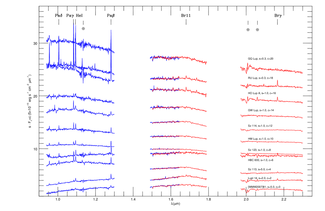
Figure 10: SofI near-IR spectra for a few selected Lupus and Serpens sources. Different colours refer to the two SofI grisms (blue and red). Spectra are shown in flux units of $5\times 10^{-15}$ erg s^-1 cm^-2 $\mu$m^-1 and were offset by a constant $c$ and multiplied by a scale factor $s$ (both indicated) for better visualisation. Wavelength intervals heavily corrupted by atmospheric absorption were removed. The position of the main emission lines present in the covered spectral range is indicated, as well as residuals from atmospheric features.

References

- Alcalá et al. (2014) Alcalá, J. M., Natta, A., Manara, C. F., et al. 2014, A&A, 561, A2
- Alcalá et al. (2008) Alcalá, J. M., Spezzi, L., Chapman, N., et al. 2008, ApJ, 676, 427
- Alves de Oliveira & Casali (2008) Alves de Oliveira, C. & Casali, M. 2008, A&A, 485, 155
- Antoniucci et al. (2013a) Antoniucci, S., Arkharov, A. A., Di Paola, A., et al. 2013a, in Protostars and Planets VI, Heidelberg, July 15-20, 2013. Poster #2B055, 55
- Antoniucci et al. (2011) Antoniucci, S., García López, R., Nisini, B., et al. 2011, A&A, 534, A32
- Antoniucci et al. (2013b) Antoniucci, S., Lorenzetti, D., Nisini, B., & Giannini, T. 2013b, The Astronomer’s Telegram, 4712, 1
- Antoniucci et al. (2008) Antoniucci, S., Nisini, B., Giannini, T., & Lorenzetti, D. 2008, A&A, 479, 503
- Calvet et al. (2000) Calvet, N., Hartmann, L., & Strom, S. E. 2000, Protostars and Planets IV, 377
- Calvet et al. (2004) Calvet, N., Muzerolle, J., Briceño, C., et al. 2004, AJ, 128, 1294
- Caratti o Garatti et al. (2012) Caratti o Garatti, A., Garcia Lopez, R., Antoniucci, S., et al. 2012, A&A, 538, A64
- Caratti o Garatti et al. (2011) Caratti o Garatti, A., Garcia Lopez, R., Scholz, A., et al. 2011, A&A, 526, L1
- Cardelli et al. (1989) Cardelli, J. A., Clayton, G. C., & Mathis, J. S. 1989, ApJ, 345, 245
- Comeron (2008) Comeron, F. 2008, in Handbook of Star Forming Regions. vol. 2, 295-350 (2008), 295–350
- Comerón et al. (2009) Comerón, F., Spezzi, L., & López Martí, B. 2009, A&A, 500, 1045
- Costigan et al. (2012) Costigan, G., Scholz, A., Stelzer, B., et al. 2012, MNRAS, 427, 1344
- D’Odorico (1988) D’Odorico, S. 1988, The Messenger, 52, 51
- Doppmann et al. (2005) Doppmann, G. W., Greene, T. P., Covey, K. R., & Lada, C. J. 2005, AJ, 130, 1145
- Edwards et al. (2006) Edwards, S., Fischer, W., Hillenbrand, L., & Kwan, J. 2006, ApJ, 646, 319
- Ercolano et al. (2014) Ercolano, B., Mayr, D., Owen, J. E., Rosotti, G., & Manara, C. F. 2014, MNRAS, 439, 256
- Evans et al. (2009) Evans, N. J., Dunham, M. M., Jørgensen, J. K., et al. 2009, ApJS, 181, 321
- Fang et al. (2009) Fang, M., van Boekel, R., Wang, W., et al. 2009, A&A, 504, 461
- Garcia Lopez et al. (2011) Garcia Lopez, R., Nisini, B., Antoniucci, S., et al. 2011, A&A, 534, A99
- Gorlova et al. (2010) Gorlova, N., Steinhauer, A., & Lada, E. 2010, ApJ, 716, 634
- Gorti et al. (2009) Gorti, U., Dullemond, C. P., & Hollenbach, D. 2009, ApJ, 705, 1237
- Greene et al. (1994) Greene, T. P., Wilking, B. A., Andre, P., Young, E. T., & Lada, C. J. 1994, ApJ, 434, 614
- Gullbring et al. (1998) Gullbring, E., Hartmann, L., Briceno, C., & Calvet, N. 1998, ApJ, 492, 323
- Hartmann et al. (1998) Hartmann, L., Calvet, N., Gullbring, E., & D’Alessio, P. 1998, ApJ, 495, 385
- Hauschildt et al. (1999) Hauschildt, P. H., Allard, F., & Baron, E. 1999, ApJ, 512, 377
- Herczeg & Hillenbrand (2008) Herczeg, G. J. & Hillenbrand, L. A. 2008, ApJ, 681, 594
- Hughes et al. (1994) Hughes, J., Hartigan, P., Krautter, J., & Kelemen, J. 1994, AJ, 108, 1071
- Isella et al. (2009) Isella, A., Carpenter, J. M., & Sargent, A. I. 2009, ApJ, 701, 260
- Isobe et al. (1990) Isobe, T., Feigelson, E. D., Akritas, M. G., & Babu, G. J. 1990, ApJ, 364, 104
- Lada & Wilking (1984) Lada, C. J. & Wilking, B. A. 1984, ApJ, 287, 610
- Lorenzetti et al. (2012) Lorenzetti, D., Antoniucci, S., Giannini, T., et al. 2012, ApJ, 749, 188
- Luhman (2007) Luhman, K. L. 2007, ApJS, 173, 104
- Merín et al. (2008) Merín, B., Jørgensen, J., Spezzi, L., et al. 2008, ApJS, 177, 551
- Mortier et al. (2011) Mortier, A., Oliveira, I., & van Dishoeck, E. F. 2011, MNRAS, 418, 1194
- Morwood (1997) Morwood, A. 1997, The Messenger, 88, 11
- Muzerolle et al. (2000) Muzerolle, J., Calvet, N., Briceño, C., Hartmann, L., & Hillenbrand, L. 2000, ApJ, 535, L47
- Muzerolle et al. (1998) Muzerolle, J., Hartmann, L., & Calvet, N. 1998, AJ, 116, 2965
- Muzerolle et al. (2005) Muzerolle, J., Luhman, K. L., Briceño, C., Hartmann, L., & Calvet, N. 2005, ApJ, 625, 906
- Natta et al. (2004) Natta, A., Testi, L., Muzerolle, J., et al. 2004, A&A, 424, 603
- Natta et al. (2006) Natta, A., Testi, L., & Randich, S. 2006, A&A, 452, 245
- Nisini et al. (2005a) Nisini, B., Antoniucci, S., Giannini, T., & Lorenzetti, D. 2005a, A&A, 429, 543
- Nisini et al. (2005b) Nisini, B., Bacciotti, F., Giannini, T., et al. 2005b, A&A, 441, 159
- Oliveira et al. (2009) Oliveira, I., Merín, B., Pontoppidan, K. M., et al. 2009, ApJ, 691, 672
- Owen et al. (2012) Owen, J. E., Clarke, C. J., & Ercolano, B. 2012, MNRAS, 422, 1880
- Owen et al. (2011) Owen, J. E., Ercolano, B., & Clarke, C. J. 2011, MNRAS, 412, 13
- Podio et al. (2006) Podio, L., Bacciotti, F., Nisini, B., et al. 2006, A&A, 456, 189
- Rieke & Lebofsky (1985) Rieke, G. H. & Lebofsky, M. J. 1985, ApJ, 288, 618
- Rigliaco et al. (2011) Rigliaco, E., Natta, A., Randich, S., Testi, L., & Biazzo, K. 2011, A&A, 525, A47+
- Rigliaco et al. (2012) Rigliaco, E., Natta, A., Testi, L., et al. 2012, A&A, 548, A56
- Shenavrin et al. (2012) Shenavrin, V. I., Grinin, V. P., Rostopchina-Shakhovskaja, A. N., Demidova, T. V., & Shakhovskoi, D. N. 2012, Astronomy Reports, 56, 379
- Sicilia-Aguilar et al. (2006) Sicilia-Aguilar, A., Hartmann, L. W., Fürész, G., et al. 2006, AJ, 132, 2135
- Sicilia-Aguilar et al. (2010) Sicilia-Aguilar, A., Henning, T., & Hartmann, L. W. 2010, ApJ, 710, 597
- Siess et al. (2000) Siess, L., Dufour, E., & Forestini, M. 2000, A&A, 358, 593
- Siess et al. (1999) Siess, L., Forestini, M., & Bertout, C. 1999, A&A, 342, 480
- Skrutskie et al. (2006) Skrutskie, M. F., Cutri, R. M., Stiening, R., et al. 2006, AJ, 131, 1163
- Spezzi et al. (2008) Spezzi, L., Alcalá, J. M., Covino, E., et al. 2008, ApJ, 680, 1295
- Straižys et al. (1996) Straižys, V., Černis, K., & Bartašiūtė, S. 1996, Baltic Astronomy, 5, 125
- Straižys et al. (2003) Straižys, V., Černis, K., & Bartašiūtė, S. 2003, A&A, 405, 585
- Tarenghi & Wilson (1989) Tarenghi, M. & Wilson, R. N. 1989, in Society of Photo-Optical Instrumentation Engineers (SPIE) Conference Series, Vol. 1114, Society of Photo-Optical Instrumentation Engineers (SPIE) Conference Series, ed. F. J. Roddier, 302–313
- Tilling et al. (2008) Tilling, I., Clarke, C. J., Pringle, J. E., & Tout, C. A. 2008, MNRAS, 385, 1530
- van Kempen et al. (2007) van Kempen, T. A., van Dishoeck, E. F., Brinch, C., & Hogerheijde, M. R. 2007, A&A, 461, 983
- Vorobyov & Basu (2006) Vorobyov, E. I. & Basu, S. 2006, ApJ, 650, 956
- White et al. (2007) White, R. J., Greene, T. P., Doppmann, G. W., Covey, K. R., & Hillenbrand, L. A. 2007, in Protostars and Planets V, ed. B. Reipurth, D. Jewitt, & K. Keil, 117–132
- Winston et al. (2009) Winston, E., Megeath, S. T., Wolk, S. J., et al. 2009, AJ, 137, 4777
- Winston et al. (2007) Winston, E., Megeath, S. T., Wolk, S. J., et al. 2007, ApJ, 669, 493