A Note on the Maximum Number of Zeros of $r(z)-\overline{z}$

Abstract

An important theorem of Khavinson & Neumann (Proc. Amer. Math. Soc. 134(4), 2006) states that the complex harmonic function $r(z)-\overline{z}$, where $r$ is a rational function of degree $n\geq 2$, has at most $5(n-1)$ zeros. In this note we resolve a slight inaccuracy in their proof and in addition we show that for certain functions of the form $r(z)-\overline{z}$ no more than $5(n-1)-1$ zeros can occur. Moreover, we show that $r(z)-\overline{z}$ is regular, if it has the maximal number of zeros.

1 Introduction

Let $r=\frac{p}{q}$ be a complex rational function of degree

$$n=\deg(r)\mathrel{\mathop{:}}=\max\{\deg(p),\deg(q)\}.$$

Here and in the sequel the polynomials $p$ and $q$ are always assumed to be coprime. We then say that the rational harmonic function

$$f(z)\mathrel{\mathop{:}}=r(z)-\overline{z}$$ (1)

is of degree $n$, too. Such functions have an interesting application in gravitional microlensing; see the introductory overview article of Khavinson & Neumann [6]. They also play a role in the matrix theory problem of expressing certain adjoints of diagonalizable matrices as rational functions of the matrix [7].

An important theorem of Khavinson & Neumann [5, Theorem 1] states that a rational harmonic function (1) of degree $n\geq 2$ has at most $5(n-1)$ zeros. In this note we give an alternative proof of their result (the differences to the original proof are discussed in Remark 2.8). Moreover, we show that a slightly better bound can be given if one takes into account the individual degrees of the numerator and denominator polynomials. In order to state our main result, we recall that a zero $z_{0}$ of $f$ is called sense-preserving if $|r^{\prime}(z_{0})|>1$, sense-reversing if $|r^{\prime}(z_{0})|<1$, and singular if $|r^{\prime}(z_{0})|=1$; see [10].

Theorem 1.1

A rational harmonic function $f(z)=r(z)-\overline{z}$ of degree $n\geq 2$ has at most $3(n-1)$ sense-preserving zeros, and at most $2(n-1)$ sense-reversing or singular zeros. Moreover, if $r=\tfrac{p}{q}$ with $\deg(p)>\deg(q)$, then $f$ has at most $5(n-1)-1$ zeros.

The first part of this theorem was already stated in [5, Theorem 1 and Proposition 1] (see also [1, Appendix B], where several extensions to this bound are presented). Our proof in the next section employs similar techniques as the one in [5], but it avoids a subtle inaccuracy in the argument, which we will explain next.

If $f(z)=r(z)-\overline{z}$ has no singular zero, then $f$ as well as $r$ are called regular. In the proof of the Main Lemma in [5], part (2), it is implicitly assumed that if $f(z)=r(z)-\overline{z}$ is regular, then the function

$$F(w)=\tfrac{1}{r(\frac{1}{w})}-\overline{w}$$

is regular as well. However, this implication is in general not correct. For example, consider the rational harmonic function $f(z)=z+\tfrac{1}{z}-\overline{z}$. Clearly, $0$ is not a zero of $f$, so that we have

$$f(z)=0\;\Leftrightarrow\;z^{2}+1=|z|^{2},$$

and hence $f$ has (only) the two zeros $\pm\tfrac{i}{\sqrt{2}}$. Since $|r^{\prime}(\pm\tfrac{i}{\sqrt{2}})|=3>1$, the function $f$ is regular. Now consider

$$F(w)=\tfrac{1}{r(\frac{1}{w})}-\overline{w}=\tfrac{w}{1+w^{2}}-\overline{w}=\mathrel{\mathop{:}}R(w)-\overline{w}.$$ (2)

Then $F(0)=0$, and $|R^{\prime}(0)|=1$ shows that $0$ is a singular zero of $F$.

In Section 2 we give a new proof of Theorem 1.1. In Section 3 we further show that $r(z)-\overline{z}$ has no singular zeros, if it has the maximal number of zeros as stated in Theorem 1.1.

2 Proof of Theorem 1.1

In order to prove Theorem 1.1 we need some preliminary results. First note that the function $R$ defined in (2) can be written as

$$R(w)=\overline{T}\circ r\circ T^{-1}(w),$$ (3)

where $w=T(z)=\tfrac{1}{z}$ is a Möbius transformation. More generally, we say that for a rational function $r(z)$ and any given Möbius transformation $T(z)$, a function $R(w)$ of the form (3) is a co-conjugate of $r(z)$. Here $\overline{T}(z)$ denotes the Möbius transformation obtained from $T(z)$ by conjugating all the coefficients. Co-conjugates maintain the number and sense of zeros of $r(z)-\overline{z}$, as we show next.

Proposition 2.1

Let $r(z)$ be rational and of degree $n\geq 1$, and let $T(z)=\frac{az+b}{cz+d}$ be a Möbius transformation. Then $R(w)=\overline{T}\circ r\circ T^{-1}(w)$ is a rational function of degree $n$ and we have:

1. $r(z)=\overline{z}$ if and only if $R(w)=\overline{w}$, for all $z\in\mathbb{C}$ with $w=T(z)\neq\infty$. In that case, if $r(z)=\overline{z}$, we have $|r^{\prime}(z)|=|R^{\prime}(w)|$.

2. Writing $r=\tfrac{p}{q}$ with $p(z)=\sum_{k=0}^{n}p_{k}z^{k}$ and $q(z)=\sum_{k=0}^{n}q_{k}z^{k}$, $R$ has the representation

   $$R(w)=\frac{\sum_{k=0}^{n}(\overline{a}p_{k}+\overline{b}q_{k})(dw-b)^{k}(a-cw)^{n-k}}{\sum_{k=0}^{n}(\overline{c}p_{k}+\overline{d}q_{k})(dw-b)^{k}(a-cw)^{n-k}}.$$ (4)

The degree of $R$ can be seen from the degree formula $\deg(r\circ s)=\deg(r)\deg(s)$ for non-constant rational functions; see [3, p. 32]. The first claim can be seen from the computations

$$r(z)=\overline{z}\Leftrightarrow(\overline{T}\circ r)(z)=\overline{T}(\overline{z})=\overline{T(z)}\Leftrightarrow R(w)=\overline{w},$$

and

$$R^{\prime}(w)=\overline{T}^{\prime}(r(z))r^{\prime}(z)(T^{-1})^{\prime}(w)=\overline{T}^{\prime}(\overline{z})r^{\prime}(z)\tfrac{1}{T^{\prime}(z)}=\tfrac{\overline{T^{\prime}(z)}}{T^{\prime}(z)}r^{\prime}(z).$$

For the second claim, note that $T^{-1}(w)=\tfrac{dw-b}{a-cw}$, so that we have

$$r(T^{-1}(w))=\frac{\sum_{k=0}^{n}p_{k}(dw-b)^{k}(a-cw)^{n-k}}{\sum_{k=0}^{n}q_{k}(dw-b)^{k}(a-cw)^{n-k}},$$

from which we see that $R(w)=\overline{T}(r(T^{-1}(w)))$ has the form (4).

In our proof of Theorem 1.1 we also need the winding of a complex function along a curve, and indices of zeros and poles of harmonic functions (sometimes called order, or multiplicity). Here we only give the most relevant definitions. A compact summary of these concepts is given in [10, Section 2], see also [2] and [11, p. 29] (where the winding is called “degree”).

Let $\Gamma$ be a rectifiable curve with parametrization $\gamma:[a,b]\to\Gamma$. Let $f:\Gamma\to\mathbb{C}$ be a continuous function with no zeros on $\Gamma$. Let $\arg f(z)$ denote a continuous branch of the argument of $f$ on $\Gamma$. The winding (or rotation) of $f(z)$ on the curve $\Gamma$ is defined as

$$V(f;\Gamma)\mathrel{\mathop{:}}=\tfrac{1}{2\pi}(\arg f(\gamma(b))-\arg f(\gamma(a)))$$

The winding is independent of the choice of the branch of $\arg f(z)$. Let $z_{0}$ be a zero or pole of $f(z)=r(z)-\overline{z}$. Denote by $\Gamma$ a circle around $z_{0}$ not containing any further zeros or poles of $f$. Then the Poincaré index of $f$ at $z_{0}$ is defined as

$$\operatorname{ind}(z_{0};f)\mathrel{\mathop{:}}=V(f;\Gamma).$$

The Poincaré index is independent of the choice of $\Gamma$.

Moreover, we will use the following results in our proof.

Proposition 2.2 ([10, Proposition 2.7])

Let $f(z)=r(z)-\overline{z}$ be a rational harmonic function with $\deg(r)\geq 2$. The indices of $f$ at $z_{0}$ can be summarized as follows:

1. If $z_{0}$ is a sense-preserving zero of $f$, then $\operatorname{ind}(z_{0};f)=1$.

2. If $z_{0}$ is a sense-reversing zero of $f$, then $\operatorname{ind}(z_{0};f)=-1$.

3. If $z_{0}$ is a pole of $r$ of order $m$, then $\operatorname{ind}(z_{0};f)=-m$.

Proposition 2.3 ([5, Proposition 1])

A rational harmonic function $f(z)=r(z)-\overline{z}$ of degree $n\geq 2$ has at most $2(n-1)$ sense-reversing or singular zeros.

Lemma 2.4 ([5, Lemma])

If $r$ is rational and of degree at least $2$, then the set of complex numbers $c$ for which $r-c$ is regular, is open and dense in $\mathbb{C}$.

A useful application of the preceeding “density lemma” emerges when combined with the continuity of the non-singular zeros of harmonic functions. In the following we call $f$ sense-preserving on an open subset $U$, if $|r^{\prime}(z)|>1$ for all $z\in U$ (similarly for sense-reversing).

Lemma 2.5

Let $f(z)=r(z)-\overline{z}$ with $\deg(r)\geq 2$. Then for every sufficiently small $\varepsilon>0$ there exists $\delta>0$ such such that for $|c|<\delta$ holds: For every sense-preserving zero $z_{0}$ of $f$, the perturbed function $f-c$ has exactly one zero $z_{0}^{\prime}$ in $\{z:|z-z_{0}|<\varepsilon\}$, which is again sense-preserving. The same applies to sense-reversing zeros.

In particular the function $f-c$ has at least as many sense-preserving (and sense-reversing) zeros as $f$.

Let $\Omega_{+}=\{z:|r^{\prime}(z)|>1\}$ be the set where $f$ is sense-preserving. Denote the sense-preserving zeros of $f$ by $z_{1},\ldots,z_{n_{+}}$. Let $\varepsilon>0$ be sufficiently small such that

1. all disks $\{z:|z-z_{j}|\leq\varepsilon\}$ are mutually disjoint and contained in $\Omega_{+}$,

2. $f$ has no zero or pole in each $\{z:0<|z-z_{j}|\leq\varepsilon\}$. (This is possible, since the zeros and poles of $f$ are isolated.)

Fix $j\in\{1,\ldots,n_{+}\}$. Set $\gamma_{j}=\{z:|z-z_{j}|=\varepsilon\}$ and let $\delta_{j}=\min_{z\in\gamma_{j}}|f(z)|>0$. Then, for any $|c|<\delta_{j}$ we have

$$|f-(f-c)|=|c|<\delta_{j}\leq|f|+|f-c|\quad\text{ on }\gamma_{j}.$$

Rouché’s theorem shows $V(f-c;\gamma_{j})=V(f;\gamma_{j})=+1$, so $f-c$ (again sense-preserving on $\Omega_{+}$) has exactly one sense-preserving zero interior to $\gamma_{j}$ (Proposition 2.2 combined with the argument principle [4]). The same applies to sense-reversing zeros (by considering the set $\Omega_{-}=\{z:|r^{\prime}(z)|<1\}$). Taking $\delta$ as the minimum of all $\delta_{j}$ completes the proof.

arxiv [Proof of Theorem 1.1] springer [of Theorem 1.1] Let us denote

$$r=\tfrac{p}{q},\quad p(z)=\sum_{k=0}^{n}p_{k}z^{k},\quad q(z)=\sum_{k=0}^{n}q_{k}z^{k},$$

and let $n_{+},n_{0},n_{-}$ be the number of sense-preserving, singular, sense-reversing zeros of $f$, respectively. Sometimes we make the dependence on $f$ explicit by writing $n_{+}(f)$ etc.

By Proposition 2.3, $n_{-,0}\mathrel{\mathop{:}}=n_{-}+n_{0}\leq 2(n-1)$. It therefore remains to show that $n_{+}\leq 3(n-1)$ and to show that $f$ has at most $5(n-1)-1$ zeros when $\deg(p)>\deg(q)$. We divide the proof in four steps.

Step 1: Let $r$ be regular with $\deg(p)\leq\deg(q)=n$, so the number of singular zeros is $n_{0}=0$. Let $\gamma$ be a circle containing all zeros and poles of $f$. In this case, since $r$ is bounded for $z\to\infty$, we have

$$|\overline{z}-f(z)|=|r(z)|\leq C<|\overline{z}|+|f(z)|,\quad z\in\gamma,$$

provided that $\gamma$ is sufficiently large. Rouché’s theorem [10, Theorem 2.3] implies $V(f;\gamma)=V(\overline{z};\gamma)=-1$. Applying the argument principle for complex-valued harmonic functions yields

$$-1=V(f;\gamma)=\sum_{z_{j}:f(z_{j})=0}\operatorname{ind}(z_{j};f)+\sum_{z_{j}:q(z_{j})=0}\operatorname{ind}(z_{j};f)=n_{+}-n_{-}-n,$$

where we used Proposition 2.2. In particular, the sum of the orders of the poles of $f$ is equal to $\deg(q)=n$. By Proposition 2.3 we have $n_{-}\leq 2(n-1)$. Thus,

$$n_{+}=n-1+n_{-}\leq n-1+2(n-1)=3(n-1).$$

Step 2: Let $\deg(p)\leq\deg(q)=n$. If $r$ is regular, we are done by Step 1, so assume that $r$ is not regular. By Lemma 2.4 there exists a sequence $c_{k}\in\mathbb{C}$ such that $r_{k}(z)\mathrel{\mathop{:}}=r(z)-c_{k}$ are regular and $c_{k}\to 0$. Then $r_{k}$ satisfies the conditions of Step 1 and, setting $f_{k}(z)\mathrel{\mathop{:}}=r_{k}(z)-\overline{z}$, we have $n_{+}(f_{k})\leq 3(n-1)$ by Step 1. For sufficiently small $|c_{k}|$, Lemma 2.5 shows that the function $f_{k}=f-c_{k}$ has at least as many sense-preserving zeros as $f$, that is, $n_{+}(f)\leq n_{+}(f_{k})\leq 3(n-1)$.

Step 3: Let $n=\deg(p)>\deg(q)$ and $p(0)\neq 0$. In this case we have $p_{n}\neq 0$, $p_{0}\neq 0$ and $q_{n}=0$. Let $w=T(z)=\frac{1}{z}$, then

$$R(w)=\overline{T}\circ r\circ T^{-1}(w)=\tfrac{1}{r(\frac{1}{w})}=\frac{\sum_{k=0}^{n}q_{k}w^{n-k}}{\sum_{k=0}^{n}p_{k}w^{n-k}},$$

which can be seen from (4). Since $p_{0}\neq 0$, we see that $F(w)=R(w)-\overline{w}$ satisfies the conditions in Step 2. Thus, $n_{+}(F)\leq 3(n-1)$ and $n_{-,0}(F)\leq 2(n-1)$.

Since $f(0)=\frac{p(0)}{q(0)}\neq 0$, every zero $z_{j}$ of $f$ gives rise to a zero $w_{j}=T(z_{j})$ of $F$, and every zero $0\neq w_{j}$ of $F$ corresponds to a zero $z_{j}=\frac{1}{w_{j}}$ of $f$; see Proposition 2.1. Since the senses of the zeros are preserved under the co-conjugation with $T$, we find

$$n_{+}(f)\leq n_{+}(F)\leq 3(n-1)\quad\text{ and }\quad n_{-,0}(f)\leq n_{-,0}(F)\leq 2(n-1).$$

Notice that $F(0)=0$, since $q_{n}=0$. This zero of $F$ has no corresponding zero of $f$, so that $f$ has at most $5(n-1)-1$ zeros.

Step 4: Let $n=\deg(p)>\deg(q)$ and $p(0)=0$. In that case we have $p_{n}\neq 0$, $q_{n}=0$ and $p_{0}=0$. Let $b\in\mathbb{C}$ satisfy $r(b)\neq\overline{b}$. With the Möbius transformation $T(z)=z-b$ we consider

$$R(w)=\overline{T}\circ r\circ T^{-1}(w)=\frac{\sum_{k=0}^{n}(p_{k}+-\overline{b}q_{k})(w+b)^{k}}{\sum_{k=0}^{n}q_{k}(w+b)^{k}};$$

see Proposition 2.1. The coefficient of $w^{n}$ in the numerator of $R$ is $p_{n}-\overline{b}q_{n}=p_{n}\neq 0$, and in the denominator it is $q_{n}=0$. Further, the constant term of the numerator of $R$ is

$$\sum_{k=0}^{n}(p_{k}-\overline{b}q_{k})b^{k}=p(b)-\overline{b}q(b)\neq 0,$$

since $r(b)\neq\overline{b}$. Thus $F(w)\mathrel{\mathop{:}}=R(w)-\overline{w}$ satisfies the conditions in Step 3, so that

$$n_{-,0}(F)\leq 2(n-1)\quad\text{and}\quad n_{+}(F)\leq 3(n-1),$$

and $F$ has at most $5(n-1)-1$ zeros.

Proposition 2.1 implies that $r(z)=\overline{z}$ if and only if $R(w)=\overline{w}$, where $w=T(z)$. Thus $f$ and $F$ have the same number of zeros, and all corresponding zeros have the same sense (or are singular). Hence $n_{-,0}(f)=n_{-,0}(F)\leq 2(n-1)$ and $n_{+}(f)=n_{+}(F)\leq 3(n-1)$, and the total number of zeros of $f$ is bounded by $5(n-1)-1$.

Remark 2.6

Let $f(z)=\frac{p(z)}{q(z)}-\overline{z}$ with $\deg(p)>\deg(q)$, so that $f$ has at most $5(n-1)-1$ zeros. Then the point $\infty$ in $\hat{\mathbb{C}}$ can be regarded as the “missing solution” to $r(z)=\overline{z}$. However, the point infinity can not be a zero of the function $r(z)-\overline{z}$, see [5, p. 1078].

Remark 2.7

In Step 3 in the above proof, one can infer the type of the zero $w=0$ of $F$. In this step $p_{n}\neq 0$ and $q_{n}=0$. We compute

$$R^{\prime}(w)=\tfrac{-r^{\prime}(\frac{1}{w})\frac{-1}{w^{2}}}{r(\frac{1}{w})^{2}}=r^{\prime}(z)\tfrac{z^{2}}{r(z)^{2}}=\tfrac{(p^{\prime}(z)q(z)-p(z)q^{\prime}(z))z^{2}}{p(z)^{2}}.$$

Note that $z^{2n}$ is the highest power of $z$ that may occur in both numerator and denominator. The coefficient of $z^{2n}$ in the denominator is $p_{n}^{2}$, and in the numerator it is

$$np_{n}q_{n-1}-p_{n}q_{n-1}(n-1)=p_{n}q_{n-1},$$

which yields

$$R^{\prime}(0)=\lim_{w\to 0}R^{\prime}(w)=\lim_{z\to\infty}\tfrac{(p^{\prime}(z)q(z)-p(z)q^{\prime}(z))z^{2}}{p(z)^{2}}=\tfrac{q_{n-1}}{p_{n}}.$$

This shows that $w=0$ may be a sense-preserving, sense-reversing or singular zero of $F$.

Remark 2.8

Let us briefly discuss how our proof of Theorem 1.1 differs from the original proof of Khavinson & Neumann in [5]. A major ingredient in both proofs is Proposition 2.3, due to Khavinson & Neumann, which bounds the number of sense-reversing and singular zeros. Because of this result it only remains to bound the number of sense-preserving zeros. Here the two main technical challenges are (i) dealing with singular zeros, and (ii) the slightly different behavior of rational functions $f(z)=\frac{p(z)}{q(z)}-\overline{z}$ with $\deg(p)\leq\deg(q)$ and $\deg(p)>\deg(q)$. The main difference between the two proofs is the order in which (i) and (ii) are handled. While Khavinson & Neumann first resolve (ii) under the assumption that all zeros are regular, and then apply the density lemma (Lemma 2.4) to resolve (i), our proof first treats the case $\deg(p)\leq\deg(q)$, using the density lemma (steps $1$ and $2$), and then transfers the result to the other case using Proposition 2.1 (steps $3$ and $4$). By this order we avoid a transformation of variables which may introduce singular zeros at a stage of the proof where this case is not covered.

The bounds in Theorem 1.1 are sharp. If $f(z)=r(z)-\overline{z}$ of degree $n\geq 2$ attains the maximal number of $5(n-1)$ zeros, we call $f$ and $r$ extremal. Examples of extremal functions were constructed by Rhie [9]. She considered the function

$$f(z)=\tfrac{z^{n-1}}{z^{n}-a^{n}}-\overline{z}$$ (5)

which is extremal for degree $n=2,3$ for a special value of $a\in(0,1)$, and the function

$$f(z)=(1-\varepsilon)\tfrac{z^{n-1}}{z^{n}-a^{n}}+\tfrac{\varepsilon}{z}-\overline{z}=\tfrac{z^{n}-\varepsilon a^{n}}{z^{n+1}-a^{n}z},$$ (6)

of degree $n+1$ which is extremal for $n\geq 3$, provided that $\varepsilon$ is sufficiently small. See [8] for a rigorous analysis of admissible parameters $a$ and $\varepsilon$ such that these functions are indeed extremal. Note that the rational function in (6) is a convex combination of the rational function in (5) and a pole located at a zero of (5). This general construction principle for extremal functions has been studied in detail in [10].

A phase portrait (see [13, 12] and [10, Section 4]) of an extremal function of the form (6) with $n=4$, and $\varepsilon=0.04$ is shown in Figure 1 (left).

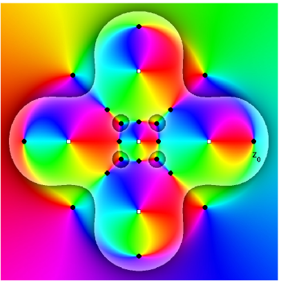
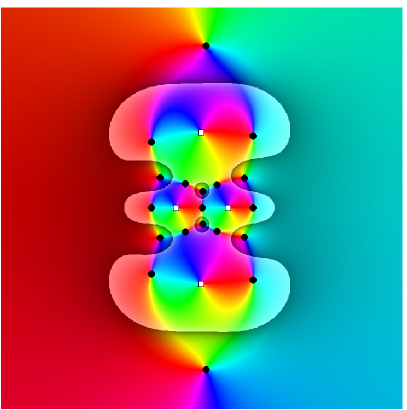
Figure 1: Phase portrais of (6) (left), and of (7) (right). Each image shows a part of the domain of the corresponding function. By indentifying the unit circle with the standard HSV color wheel, each point in the domain is colored according to the phase $e^{i\arg{f(z)}}$ of the function value at that point (see [12]). The brightened regions indicate the parts of the domain where the function is sense-preserving. Black disks denote zeros, white squares poles. Both functions are of degree five, and have $20$ and $19$ zeros, respectively, which is the maximum possible number in each case.

We show that for rational functions with $\deg(p)>\deg(q)$ the new bound from Theorem 1.1 is also sharp. Let $r$ be the any of the extremal rational functions from (5) and (6). Let $z_{0}$ be any zero of $f(z)=r(z)-\overline{z}$ and consider the co-conjugate of $r$ with $w=T(z)=\tfrac{1}{z-z_{0}}$:

$$R(w)=\overline{T}\circ r\circ T^{-1}(w)=\tfrac{1}{r(\frac{1}{w}+z_{0})-\overline{z}_{0}}.$$

From Proposition 2.1 it is easy to see that the numerator of $R$ has degree $\deg(r)$ and the denominator has degree (at most) $\deg(r)-1$. Further the zeros of

$$F(w)=R(w)-\overline{w}$$ (7)

are exactly the images of the zeros ($\neq z_{0}$) of $f(z)=r(z)-\overline{z}$, so that $F$ has $5(\deg(R)-1)-1$ zeros. Figure 1 (right) illustrates this construction for $n=4$, where $z_{0}$ is the rightmost zero of $f$ in the left phase portrait.

3 Extremal Rational Harmonic Functions are Regular

In this section we will show that functions $f(z)=r(z)-\overline{z}$ that attain the maximum number of zeros as stated in Theorem 1.1 are, surprisingly, guaranteed to be regular.

Theorem 3.1

Let $r=\frac{p}{q}$ be a rational function of degree $n\geq 2$ and set $f(z)=r(z)-\overline{z}$. If

1. $f$ has $5(n-1)$ zeros, or

2. $\deg(p)>\deg(q)$ and $f$ has $5(n-1)-1$ zeros,

then none of the zeros are singular.

(i) Let $\Omega_{+}\mathrel{\mathop{:}}=\{z:|r^{\prime}(z)|>1\}$ be the set where $f$ is sense-preserving. Denote by $n_{+}$ the number of zeros of $f$ in $\Omega_{+}$ and by $n_{-,0}$ the number of zeros of $f$ in $\{z:|r^{\prime}(z)|\leq 1\}$. Since $f$ has $5(n-1)$ zeros, Theorem 1.1 implies

$$n_{+}=3(n-1),\quad n_{-,0}=2(n-1).$$

Suppose $f$ has a singular zero $z_{0}$. Let $z_{1},\ldots,z_{n_{+}}$ be the $n_{+}=3(n-1)$ zeros of $f$ in $\Omega_{+}$. Let $\varepsilon>0$ be such that the disks $\{z:|z-z_{j}|\leq\varepsilon\}$ do not intersect for $0\leq j\leq n_{+}$, and are contained in $\Omega_{+}$ for $1\leq j\leq n_{+}$. By Lemma 2.5 applied to $f$ on $\Omega_{+}$ there exists $\delta>0$ such that for all $|c|<\delta$ the function $f-c$ has exactly one zero in each $\varepsilon$-disk $D_{\varepsilon}(z_{j})=\{z:|z-z_{j}|<\varepsilon\}$, $1\leq j\leq n_{+}$.

Now, since $f(z_{0})=0$ and $f$ is continuous near $z_{0}$, there exists $0<\eta\leq\varepsilon$ such that $|f(z)|<\delta$ in $D_{\eta}(z_{0})=\{z:|z-z_{0}|<\eta\}$. Further, there exists $\zeta\in D_{\eta}(z_{0})\cap\Omega_{+}$. Indeed, assume the contrary, then $|r^{\prime}(z)|\leq 1$ in $D_{\eta}(z_{0})$ and $|r^{\prime}(z_{0})|=1$, which implies that $r^{\prime}$ is constant by the maximum modulus theorem, a contradiction to $\deg(r)\geq 2$.

Finally, consider the function $F(z)\mathrel{\mathop{:}}=f(z)-f(\zeta)$. Since $|f(\zeta)|<\delta$, $F$ has exactly one zero in each disk $D_{\varepsilon}(z_{j})$, $1\leq j\leq n_{+}$, and further $F(\zeta)=0$. Thus $F$ has $n_{+}+1=3(n-1)+1$ distinct sense-preserving zeros in $\Omega_{+}$, in contradiction to Theorem 1.1. Therefore $f$ has no singular zeros.

(ii) We reduce this case to the previous one. Let $b\in\mathbb{C}$ such that $r(b)\neq\overline{b}$, and define the Möbius transformation $w=T(z)=\frac{1}{z-b}$. Consider the co-conjugate $R=\overline{T}\circ r\circ T^{-1}$ and $F(w)=R(w)-\overline{w}$. By Proposition 2.1, all $5(n-1)-1$ zeros of $f$ transform to zeros of $F$ with $|r^{\prime}(z)|=|R^{\prime}(w)|$, so that the senses are preserved. Note that none of the zeros of $f$ is mapped to $0$ under $T$. However, (4) and $n=\deg(p)>\deg(q)$ imply $R(0)=\frac{q_{n}}{p_{n}}=0$, so that we have $F(0)=0$. Thus $F$ has a total number of $5(n-1)$ zeros, none of which is singular by the first part. Hence none of the zeros of $f$ are singular.

Ackowledgements

We would like to thank Dmitry Khavinson for pointing out reference [1] to us. We are grateful to the anonymous referee for the careful reading of the manuscript, and many valuable remarks.

Robert Luce’s work is supported by Deutsche Forschungsgemeinschaft, Cluster of Excellence “UniCat”.

References

- [1] Jin H. An and N. Wyn Evans. The Chang-Refsdal lens revisited. Monthly Notices of the Royal Astronomical Society, 369(1):317–334, 2006.
- [2] Mark Benevich Balk. Polyanalytic Functions. Mathematical Research. 63. Berlin: Akademie-Verlag. 197 p. , 1991.
- [3] Alan F. Beardon. Iteration of rational functions, volume 132 of Graduate Texts in Mathematics. Springer-Verlag, New York, 1991. Complex analytic dynamical systems.
- [4] Peter Duren, Walter Hengartner, and Richard S. Laugesen. The argument principle for harmonic functions. Amer. Math. Monthly, 103(5):411–415, 1996.
- [5] Dmitry Khavinson and Genevra Neumann. On the number of zeros of certain rational harmonic functions. Proc. Amer. Math. Soc., 134(4):1077–1085 (electronic), 2006.
- [6] Dmitry Khavinson and Genevra Neumann. From the fundamental theorem of algebra to astrophysics: a “harmonious” path. Notices Amer. Math. Soc., 55(6):666–675, 2008.
- [7] Jörg Liesen. When is the adjoint of a matrix a low degree rational function in the matrix? SIAM J. Matrix Anal. Appl., 29(4):1171–1180, 2007.
- [8] Robert Luce, Olivier Sète, and Jörg Liesen. Sharp parameter bounds for certain maximal point lenses. Gen. Relativity Gravitation, 46(5):46:1736, 2014.
- [9] S. H. Rhie. n-point Gravitational Lenses with 5(n-1) Images. ArXiv Astrophysics e-prints, May 2003.
- [10] Olivier Sète, Robert Luce, and Jörg Liesen. Perturbing rational harmonic functions by poles. Computational Methods and Function Theory, pages 1–27, 2014.
- [11] T. Sheil-Small. Complex polynomials, volume 75 of Cambridge Studies in Advanced Mathematics. Cambridge University Press, Cambridge, 2002.
- [12] Elias Wegert. Visual complex functions. Birkhäuser/Springer Basel AG, Basel, 2012. An introduction with phase portraits.
- [13] Elias Wegert and Gunter Semmler. Phase plots of complex functions: a journey in illustration. Notices Am. Math. Soc., 58(6):768–780, 2011.