Millihertz Quasi-Periodic Oscillations and broad iron line from LMC X–1

Abstract

We study the temporal and energy spectral characteristics of the persistent black hole X-ray binary LMC X–1 using two XMM-Newton and a Suzaku observation. We report the discovery of low frequency ($\sim 26-29{\rm~{}mHz}$) quasi-periodic oscillations (QPOs). We also report the variablity of the broad iron K$\alpha$ line studied earlier with Suzaku. The QPOs are found to be weak with fractional $rms$ amplitude in the $\sim 1-2\%$ range and quality factor $Q\sim 2-10$. They are accompanied by weak red noise or zero-centered Lorentzian components with $rms$ variability at the $\sim 1-3\%$ level. The energy spectra consists of three varying components – multicolour disk blackbody ($kT_{in}\sim 0.7-0.9{\rm~{}keV}$), high energy power-law tail ($\Gamma\sim 2.4-3.3$) and a broad iron line at $6.4-6.9{\rm~{}keV}$. The broad iron line, the QPO and the strong power-law component are not always present. The QPOs and the broad iron line appear to be clearly detected in the presence of a strong power-law component. The broad iron line is found to be weaker when the disk is likely truncated and absent when the power-law component almost vanished. These results suggest that the QPO and the broad iron line together can be used to probe the dynamics of the accretion disk and the corona.

1 Introduction

The highly variable X-ray emission from black hole X-ray binaries (BHBs) shows a variety of quasi-periodic oscillations (QPOs) that appear as peaks of small but finite widths in the power density spectra (PDS) (Remillard et al., 1999; Lewin & van der Klis, 2006; Remillard & McClintock, 2006; Belloni, 2010; Motta et al., 2011). These QPOs can be grouped in three categories – ($i$) high frequency QPOs that occur in the frequency range of $\sim 30-100{\rm~{}Hz}$ and are generally transient (see e.g., Belloni et al., 2012), ($ii$) low frequency QPOs (LFQPOs) in the range of $0.05-30{\rm~{}Hz}$ (Casella et al., 2005; Motta et al., 2011), (iii) very low frequency ($\sim{\rm mHz}$) QPOs that have been observed in the heart-beat sources GRS 1915+105 (Morgan et al., 1997; Trudolyubov et al., 2001) and IGR J17091–3624 (Belloni et al., 2000; Altamirano et al., 2011a). Recently, mHz QPOs have also been detected from the BHBs H 1743–322 ($\sim 11{\rm~{}mHz}$; Altamirano & Strohmayer 2012) and IC X–1 ($\sim 7{\rm~{}mHz}$; Pasham & Strohmayer 2013). Some ultra-luminous X-ray sources (ULXs) also show very low frequency QPOs at $\raisebox{-2.15277pt}{$\;\stackrel{{\scriptstyle<}}{{\sim}}\;$}100{\rm~{}mHz}$, e.g., M 82 X–1 (Strohmayer & Mushotzky, 2003; Dewangan et al., 2006; Mucciarelli et al., 2006; Caballero-García et al., 2013; Pasham & Strohmayer, 2013), NGC 5408 X–1 (Dheeraj & Strohmayer, 2012), although they could be the counterpart of LFQPOs if these ULXs contain intermediate mass black holes. The LFQPOs come in varieties with three main types – Type A (weak with a few percent rms and broad peak around $8{\rm~{}Hz}$), Type B (relatively strong with $\sim 4\%$ rms and narrow peak around $6{\rm~{}Hz}$) and Type C (strong up to $16\%$ rms, narrow and variable peak) (see e.g., Casella et al., 2005).

While the exact origin of QPOs from BHBs is still a mystery, the type C LFQPOs are correlated with energy spectral properties. The centroid frequency is found to be correlated with the disk flux (Motta et al., 2011; Markwardt et al., 1999), and the rms amplitude is found to increase with energy (Casella et al., 2004; Belloni et al., 1997, 2011). It implies that the LFQPOs do not directly arise from the thermal accretion disk as the accretion disk emission does not extend to higher energies.

The evolution of black hole transients can be characterized in terms of a limited number of states viz. Low-Hard state (LHS), Hard Intermediate State (HIMS), Soft Intermediate State (SIMS), High Soft State (HSS), and the transitions between these states. The LHS is characterised by a strong dominant power-law emission with a variable slope ($\Gamma\sim 1.5-2.1$) correlated with flux and a high-energy cutoff, also variable between 60 and 120 keV (see e.g., Motta et al., 2009). In the HIMS, a softer component originating from a thermal accretion disk component contributes more to the observed emission and the power law component steepens, with an increase in the high energy cutoff value (Motta et al., 2009; Belloni et al., 2011). The SIMS is softer than the HIMS due to larger contribution of the disk emission and is characterised by low level ($\sim$a few $\%$ rms) of variability (Belloni et al., 2011). The LHS is usually associated with a steady radio-jet (Corbel et al., 2013, and references therein). In the HIMS, a type-C LFQPO is always observed, as is often the case in the brightest LHS. In the SIMS, QPOs of type A or B are often observed. In contrast, LFQPOs are generally not observed in the HSS dominated by thermal emission from accretion disks (see reviews by Remillard & McClintock, 2006; Belloni, 2010).

Hard X-ray irradiation of the thermal accretion disk can give rise to X-ray fluorescence emission lines below $10{\rm~{}keV}$ and Compton reflection hump in the $10-50{\rm~{}keV}$ band. The iron K$\alpha$ emission line, broadened by Doppler and gravitational effects near a black hole in X-ray binaries and active galactic nuclei, is proven to be one of the most important diagnostic of the inner most regions of strong gravity (see e.g., Reynolds & Nowak, 2003; Miller, 2007). The strength and extent of the red wing of the relativistic iron line is determined by the inner extent of the accretion disk which is smaller than $6r_{g}$ if the black hole is spinning, where $r_{g}=GM/c^{2}$ is the gravitational radius. For a maximally spinning black hole, the innermost stable circular orbit is $r_{ISCO}\sim r_{g}$. Indeed, the presence of broad iron lines in the X-ray spectra of both black hole X-ray binaries and AGN have been used to determine the size of the inner disk and from that to infer the black hole spin.

The production of a broad iron line depends both on the presence of an accretion disk extending to the innermost regions and a strong hard X-ray continuum illuminating the disk. The presence of LFQPOs also depends on the power-law component. This suggests that the iron K$\alpha$ line and LFQPOs are likely related though not directly. In the soft spectral states, strong iron K lines are usually not observed, due to lack of strong hard X-ray continuum (Miller, 2007). Similarly, LFQPOs are not observed in the high/soft states. The relationship between the broad iron line and the LFQPOs, their dependence on the hard X-ray continuum and the presence of an accretion disk are good tests of disk/corona geometry and the models for the origin of both the iron line and LFQPOs.

LMC X–1, located in the Large Magellanic Cloud, is a luminous and persistent black hole X-ray binary (BHB). It consists of a $10.19\pm 1.41{\rm~{}M_{\odot}}$ black hole primary and an O7 III companion orbiting each other with a $3.9$-day period (Orosz et al., 2009; Cowley et al., 1995). The companion drives a strong wind that powers the black hole with an average luminosity of $0.16L_{Edd}$ (Nowak et al., 2001; Gou et al., 2009). LMC X–1 has remained in the HSS persistently and has never been observed to undergo a transition to the LHS (Nowak et al., 2001; Ruhlen et al., 2011). The temporal properties of LMC X-1 are typical of HSS with its PDS approximately proportional to $\nu^{-1}$ and fractional root mean square variability (rms) of $\sim 7\%$ (Nowak et al., 2001). Previously, two QPOs at $75{\rm~{}mHz}$ and $142{\rm~{}mHz}$ have been reported from LMC X–1, based on Ginga observations (Ebisawa et al., 1989). However, a series of nine RXTE observations performed in 1996 (Schmidtke et al., 1999) and a long $170{\rm~{}ks}$ RXTE observation (Nowak et al., 2001) did not detect any QPO from the source. It has been suggested that the $75{\rm~{}mHz}$ and $142{\rm~{}mHz}$ QPOs detected by Ebisawa et al. (1989) is likely an artifact due to incorrect estimation of the Poisson noise level (Nowak et al., 2001). The X-ray spectrum of LMC X–1 is typical of the HSS in which the thermal disk component dominates over the power-law component (Ebisawa et al., 1989; Nowak et al., 2001; Ruhlen et al., 2011) However, spectral evolution of LMC X–1 does not follow the modified Stefan-Boltzmann relation $L_{disk}\propto T_{in}^{4}$ expected from the HSS of BHBs (see Ruhlen et al., 2011). The presence of broad iron line from LMC X–1, earlier inferred from RXTE observations (Nowak et al., 2001), has been confirmed by Steiner et al. (2012) who measured a spin $a=0.97^{+0.02}_{-0.025}$ using Suzaku observations. Steiner et al. (2012) also found a strong correlation between the relative strength of the Compton power law and the iron line flux using the RXTE observations.

In this paper, we perform timing and spectral study of LMC X–1 based on XMM-Newton and Suzaku observations and report the detection of ${\rm~{}mHz}$ QPOs and variable broad iron line. We show that the iron line and the QPO are not always present, and investigate the relationship between them. We describe the observations analysed and data reduction in Sect. 2, temporal analysis in Sect. 3, and spectral analysis in Sect. 4. We finally discuss our results in Sect. 5.

2 Observations & Data Reduction

2.1 XMM-Newton

XMM-Newton observed LMC X–1 twice: on 2000 October 21 (obsID: 0112900101; hereafter xmm-101) and 2002 September 26 (obsID:0023940401; hereafter xmm-401) for exposure times of $7.2{\rm~{}ks}$ and $40{\rm~{}ks}$, respectively. The EPIC-pn camera was operated in timing mode using the thick optical blocking filter in 2000 October and thin filter in 2002 September. The MOS cameras were operated in the full frame mode using the medium optical blocking filter in both observations. We used SAS version 12.0 and the most recent calibration database to process and filter the event data. We corrected the EPIC-pn event list for the rate-dependent charge transfer inefficiency which has been seen in the fast mode data. We checked for particle background by extracting lightcurves above $10{\rm~{}keV}$ from both EPIC-pn and MOS data. No flaring background was found in the xmm-101 data. In the xmm-401 data, the flaring particle background was present in the beginning of observation for a short interval of $\sim 1400{\rm~{}s}$ and after an elapsed time of $\sim 26{\rm~{}ks}$. We excluded these intervals of high particle background by using good time intervals created based on count rate cutoff criteria. We extracted the $10-12{\rm~{}keV}$ light curve from the EPIC-pn data and created a GTI file by selecting the intervals with the count rate $\leq 0.5{\rm~{}counts~{}s^{-1}}$. We then applied the GTI file and filtered the event list for high particle background. This resulted in the net exposures of $23.3{\rm~{}ks}$ for the xmm-401 observation. The MOS data from both observations were affected with photon pile up. So we did not use MOS data for further analysis.

In the EPIC-pn timing mode, only one CCD chip is operated. The data are collapsed into one-dimensional row of size 64 pixels or $4.4\arcmin$ and are continuously transferred along the second dimension and readout at high speed resulting in $30\mu{\rm~{}s}$ time resolution. This allows for high count rates and photon pile-up is negligible below $800{\rm~{}counts~{}s^{-1}}$. The EPIC-pn count rate of LMC X–1 was only $113{\rm~{}counts~{}s^{-1}}$. Hence, the EPIC-pn data in the timing mode were not affected with pile-up which was also verified with epatplot. We extracted the source spectra from the EPIC-pn single pixel events using a rectangular region of $15$ pixel width covering the source. We also extracted the corresponding background spectra uwing two rectangular regions of widths 10 and 5 pixels away from the source. We used the SAS tasks rmfgen and arfgen to generate the response files.

2.2 Suzaku

Suzaku observed LMC X–1 starting on 2009 July 21, 18:38 UT for $129.8{\rm~{}ks}$ (Observation ID 404061010). The observation was performed at XIS nominal pointing and the XIS were operated in the 1/4 window mode resulting in time resolution of $2{\rm~{}s}$. We used Suzaku FTOOLS version 19 and reprocessed and screened the XIS and HXD PIN data using the aepipeline and the most recent version of calibration database to produce the cleaned event lists. We checked for photon pile up in the XIS data using the ISIS tools aeattcor.sl and pile_estimate.sl. A new attitude file was created which was then applied to the XIS event lists that resulted in sharper images. An estimated, minimum pile-up fraction image was created at different levels $0.03\%$, $0.3\%$, $1\%$, $2\%$, $5\%$, $10\%$, and $20\%$. For spectral extraction from the XIS0 data, we made a circular region file with $130\arcsec$ radius and from its center excluded a rectangular region ($14.5\arcsec\times 32.3\arcsec$) with pile-up fraction $>5\%$. Similar regions were created for XIS1 and XIS3. The source spectra was extracted from these regions using xselect. We also extracted background spectra from multiple circular regions with typical sizes $\sim 60\arcsec$ away from the source. The response files were created using the tools xisrmfgen and xissimarfgen. The HXD/PIN spectral products were extracted using the tool hxdpinxbpi.

3 Temporal Analysis

We used the X-ray timing software GHATS version 1.1.0 to compute power density spectra (PDS). We begin with temporal analysis of $0.3-10{\rm~{}keV}$ XMM-Newton EPIC-pn data. The PDS for xmm-401 were created with a time binsize of $0.096{\rm~{}s}$ (Nyquist frequency of $5.2{\rm~{}Hz}$), and time segments of 4096 bins in each lightcurve. The PDS of different segments were averaged and the resulting PDS were logarithmically rebinned in frequency to improve statistics. The PDS were computed using rms normalisation (Belloni & Hasinger, 1990). The PDS for the xmm-101 data was derived using a time resolution of $60{\rm~{}ms}$ and time segments of 16384 bins in each lightcurve. The averaged and logarithmically binned PDS for xmm-101 and xmm-401 are shown in Fig. 1. The PDS of LMC X–1 is featureless red noise during xmm-101 while a clear narrow peak in addition to the red noise is seen in the xmm-401 data.

The PDS were fit using ISIS version 1.6.2-27. Unless otherwise specified, all errors on the best-fit parameters are quoted at the $90\%$ confidence level corresponding to the minimum $\chi^{2}+2.71$. The detection significance of the QPOs were calculated based on the $1\sigma$ errors corresponding to the minimum $\chi^{2}+1.0$. A constant variability power results from Poisson noise alone, therefore we first fitted a constant model to the PDS derived from the xmm-401 data. This model resulted in unsatisfatory fit ($\chi^{2}/dof=161.5/91$) with large residuals around $\sim$0.03 Hz. We then added a model for a Lorentzian-shaped QPO for the $\sim$0.03 Hz narrow feature. The parameters of the QPO model are the centroid frequency ($\nu_{qpo}$), the quality factor ($Q=\nu_{qpo}/\Delta\nu$) and the normalization (rms/mean). The constant+qpo model improved the fit to $\chi^{2}/dof=97.4/88$, and resulted in small residuals at the lowest frequencies below $0.006{\rm~{}Hz}$. Addition of a powerlaw component (plaw) resulted only in marginal improvement ($\chi^{2}/dof=91.2/86$). The QPO is detected at a very high ($6.8\sigma$) statistical significance level, computed as the ratio between the best fit normalization and its $1\sigma$ negative error. The best-fit centroid frequency is $\nu_{qpo}=2.77_{-0.12}^{+0.13}\times 10^{-2}{\rm~{}Hz}$ and the quality factor $Q=\nu_{qpo}/\Delta\nu=3.8_{-1.4}^{+3.2}$. Without the plaw component, the QPO is detected at much higher ($15.2\sigma$) significance level and the QPO parameters remained similar. For xmm-101, we found that the constant+plaw model adequately describes the PDS ($\chi^{2}/dof=106.3/106$) without any requirement for a QPO. We calculated an upper-limit on the $rms$ of a possible QPO by adding a QPO model. We fixed the QPO frequency and the quality factor to the best-fit values obtained for the xmm-401 data and varied the QPO normalization. This resulted in $\chi^{2}/dof=106.3/105$ and the $90\%$ upper-limit on the fractional rms is $1.1\%$.

To create the PDS of LMC X–1 using the Suzaku XIS data we extracted lightcurves with $2{\rm~{}s}$ bins from the XIS0, XIS1 and XIS3 cleaned data in the $0.4-9{\rm~{}keV}$ band and combined the three lightcurves. We used the xronos task powspec to generate the PDS from the combined XIS lightcurve. We divided the lightcurve in 131 segments of 1024 bins. We discarded segments with gaps and calculated the PDS from each segment without any gap and averaged the power in each frequency bin and obtained the final PDS. We fitted the PDS in the $2.5\times 10^{-4}-0.25{\rm~{}Hz}$ range derived from the Suzaku/XIS data. We used a broad Lorentzian, a powerlaw and a constant model for the continuum as it provided a better fit ($\chi^{2}/dof=694.9/506$) compared to the plaw + constant ($\chi^{2}/dof=725.9/509$). Examination of the residual showed a narrow peak at $\sim 0.027{\rm~{}Hz}$ and addition of a qpo improved the fit to $\chi^{2}/dof=671.8/503$. Thus, we again detected a QPO at high significance ($6.4\sigma$ level). The centroid of the QPO is almost at the same frequency ($\nu_{qpo}\sim 0.027$) as for the xmm-401 data, and the coherence is high ($Q\sim 4-17$). We have listed the best-fit PDS parameters for the three observations in Table 1. We have shown the PDS data and the best-fitting models in the third row of Fig. 1. We also created EPIC-pn lightcurve folded with the corresponding QPO period using the FTOOLS task efold. Fig. LABEL:fig:f2 shows the folded lightcurve.

Table 1: Best-fit model parameter PDS derived from the XMM-Newton observations xmm-401 and xmm-101, and Suzaku.

Model	Parameter	xmm-401	xmm-101	Suzaku/XIS
		const. + qpo	const + plawa	const. + plawa + lo + qpo
constant		$0.0180_{-0.0004}^{+0.0002}$	$0.0164\pm 0.0003$	$0.0212_{-0.0007}^{+0.0002}$
plaw	index	$-0.7_{-3.3}^{+0.4}$	$-0.85_{-0.16}^{+0.14}$	$-1.09_{-0.04}^{+0.11}$
	Norm ($10^{-4}$)	$1.15_{-1.11}^{+5.25}$	$4.8_{-2.4}^{+3.6}$	$2.1_{-0.2}^{+1.5}$
LO	$\nu_{L}$ ($10^{-3}{\rm~{}Hz}$)	–	–	$3.1_{-0.7}^{+0.5}$
	FWHM	–	–	$3.1_{-1.7}^{+2.8}$
	Norm ($10^{-4}$)	–	–	$4.4_{-1.7}^{+1.7}$
qpo	$\nu_{qpo}$($10^{-2}{\rm~{}Hz}$)	$2.77_{-0.12}^{+0.13}$	–	$2.67_{-0.06}^{+0.07}$
	Q	$3.8_{-1.4}^{+3.2}$	–	$9.4_{-5.0}^{+8.8}$
	rms	$0.019_{-0.003}^{+0.004}$	–	$0.008_{-0.002}^{+0.002}$
	$\chi^{2}_{min}$/dof	$91.2/86$	$106.3/106$	$671.8/503$
	$\Delta\chi^{2}$ (QPO)	$-42.0$	–	$-23.0$

$a$ plaw: power-law model
$b$ zfc: Zero-centred Lorentzian model

Table 2: Best-fit spectral parameters of LMC X–1 derived from the XMM-Newton and Suzaku observations

Component	Parameter (a)	Suzaku		xmm-401		xmm-101
		model B (b)	model C (b)	model B (b)	model C (b)	model A (b)
tbvarabs	$N_{H}$ ($10^{22}{\rm~{}cm^{-2}}$)	$1.08_{-0.24}^{+0.24}$	$1.66_{-0.18}^{+0.15}$	$1.0_{-0.2}^{+0.3}$	$1.1_{-0.2}^{+0.4}$	$<0.7$
diskbb	$kT_{in}$ (keV)	$0.79_{-0.01}^{+0.02}$	$0.77_{-0.01}^{+0.02}$	$0.65\pm 0.02$	$0.68\pm 0.01$	$0.90\pm 0.03$
	$n_{diskbb}$ (c)	$96.4_{-6.7}^{+12.9}$	$101.7_{-9.1}^{+18.9}$	$172_{-51}^{+72}$	$133.8_{-5.8}^{+4.7}$	$23.8_{-2.5}^{+5.3}$
simpl	$\Gamma$	$2.45_{-0.04}^{+0.04}$	$2.41_{-0.04}^{+0.06}$	$2.91_{-0.13}^{+0.04}$	$2.80_{-0.06}^{+0.04}$	$3.3_{-p}^{+p}$
	$f_{scr}$	$0.138_{-0.005}^{+0.004}$	$0.078_{-0.017}^{+0.014}$	$0.35_{-0.04}^{+0.02}$	$0.294_{-0.008}^{+0.019}$	$0.026_{-0.021}^{+0.014}$
reflionx	$n_{ref}~{}^{(d)}$ ($\times 10^{-7}$)	–	$1.17_{-0.16}^{+0.22}$	–	$4.5_{-3.6}^{+p}$	–
	Fe/solar	–	1 (f)	–	1 (f)	–
	$\xi$ ($\rm ergs~{}cm~{}s^{-1}$)	–	$>8360$	–	$1795_{-770}^{+1042}$	–
kdblur	$i$	–	$36.38\degr$ (f)	–	$36.38\degr$ (f)	–
	$r_{in}$ ($r_{g}$)	–	$2.38_{-0.19}^{+0.59}$	–	$>32$	–
	$r_{out}$ ($r_{g}$)	–	$400$ (f)	–	$400$ (f)	–
	$q$	–	$3.37_{-0.19}^{+0.25}$	–	$3$ (f)	–
laor	$E_{line}$ (keV)	$6.9_{-0.02}^{+p}$	–	$6.69_{-0.10}^{+0.11}$	–	–
	$r_{in}$	$2.3_{-0.1}^{+0.1}$	–	$64_{-31}^{+113}$	–	–
	$r_{out}$ ($r_{g}$)	$400$ (f)	–	$400$ (f)	–	–
	$q$	$4.5_{-0.1}^{+0.1}$	–	$3$ (f)	–	–
	$f_{line}~{}^{(e)}$	$7.9_{-1.0}^{+1.1}\times 10^{-4}$	–	$4.6_{-2.0}^{+1.7}\times 10^{-5}$	–	–
	$\chi^{2}_{min}/dof$	$839.6/731$	765.6/731	145.5/151	145.2/151	$115.8/107$
	$f_{2.5-10{\rm~{}keV}}~{}^{(f)}$	$2.4\times 10^{-10}$	$2.4\times 10^{-10}$	$2.0\times 10^{-10}$	$2.0\times 10^{-10}$	$1.0\times 10^{-10}$
	$f_{10-60{\rm~{}keV}}~{}^{(f)}$	$7.8\times 10^{-11}$	$7.8\times 10^{-11}$	–	–	–
	disk frac. (g)	$\sim 0.60$	–	$\sim 0.35$	–	$\sim 94$

($a$) $p$ indicates that the error calculations pegged at the lower/upper bounds and (f) indicates a fixed parameter.
($b$) Models A : tbvarabs$\times$diskbb$\ast$simpl; B : tbvarabs$\times$(diskbb$\ast$simpl $+$ laor); C: tbvarabs$\times$(diskbb$\ast$simpl $+$ kdblur$\ast$reflionx)
($c$) diskbb normalisation $n_{diskbb}=\left(\frac{R_{in}/{\rm km}}{D/10{\rm~{}kpc}}\right)^{2}\cos{i}$, where $R_{in}$ is an apparent inner radius, $D$ is the distance and $i$ is the inclination angle.
($d$) reflionx normalisation in units of ${\rm photons~{}cm^{-2}~{}s^{-1}~{}keV^{-1}}$ at $1{\rm~{}keV}$.
($e$) Flux of the laor line in units of ${\rm photons~{}cm^{-2}~{}s^{-1}}$.
($f$) Observed flux in units of ${\rm~{}ergs~{}cm^{-2}~{}s^{-1}}$.
($g$) Fraction of disk flux and the simpl flux in the $2-20{\rm~{}keV}$.

4 Spectral Analysis

We used ISIS version 1.6.2-27 for our spectral analysis. As before, we quote the errors on the best-fit model parameters at the $90\%$ confidence level. In all spectral fits, we used the absorption model tbvarabs (Wilms et al., 2000) with fixed abundaces as obtained by Hanke et al. (2010).

We began with the spectral fitting of the broadband Suzaku data. The broadband spectrum of LMC X–1 extracted from the same data have been studied in detail by Steiner et al. (2012) who discovered the relativistic iron K$\alpha$ line and measured the black hole spin $a_{\star}=0.97_{-0.25}^{+0.02}$. Our purpose here is to study the spectral variability of LMC X–1 using Suzaku and XMM-Newton observations. We grouped the XIS spectral data to a minimum signal-to-noise of 10 and minimum channel of 2 in each bin. This ensures a minimum counts of more than $90$ per bin. To check the cross-calibration issues between the three XIS instrument we fitted an absorbed diskbb plus powerlaw model jointly to the XIS0, XIS1 and XIS3 data in the $0.5-10{\rm~{}keV}$ band. Examination of the data to model ratio showed a discrepancy between the three XISs as large as $20\%$ below $2.5{\rm~{}keV}$. Therefore, we excluded XIS data below $2.5{\rm~{}keV}$ and used the XIS data in the $2.5-10{\rm~{}keV}$ band. The broad iron line is clearly seen in the $4-7{\rm~{}keV}$ band. There are also slight cross-calibration problems at a level of $2-3\sigma$ between the back illuminated CCDs (XIS0 and XIS3) and the front illuminated CCD (XIS1) in the iron K band. We added a $1\%$ systematic error to each of the three XIS data sets to account for possible uncertainties in the calibration of different instruments. We grouped the PIN data to a minimum signal-to-noise of 3 per bin and used the $15-70{\rm~{}keV}$ band. We fitted the XIS and PIN data jointly with the absorbed diskbb and the empirical convolution model of Comptonization simpl which gives the fraction of photons in the input seed spectrum that are upscattered into a power-law component (Steiner et al., 2009). Since simpl redistributes seed photons to higher energies, we extended the sampled energies to $1000{\rm~{}keV}$ to calculate the model. We multiplied the model with a constant component to account for variations in the relative normalization of the instruments. The constant was fixed at 1 for XIS0 and 1.16 for PIN, and varied for XIS1 and XIS3. This model (model A : tbvarabs$\times$(diskbb$\ast$simpl)) resulted in $\chi^{2}=1768.9$ for $736$ degrees of freedom (dof). The fit is poor due to the presence of a broad feature in the $4.5-7{\rm~{}keV}$ band reminiscent of relativistic iron K$\alpha$ line. To show the broad iron line clearly, we excluded the data in the $4.5-8{\rm~{}keV}$ band and refitted. This resulted in $\chi^{2}/dof=355.2/372$ with $N_{H}\sim 9.6\times 10^{21}{\rm~{}cm^{-2}}$, $\Gamma\sim 2.36$ and $f_{scr}\sim 0.12$. We then evaluated the best-fit model in the $4.5-8{\rm~{}keV}$ band. The upper-right panel in Fig. 1 shows the deviations of the observed data from the continuum model. To model the relativistic iron line, we added a laor line (model B: tbvarabs$\times$(diskbb$\ast$simpl + laor)). The laor model describes the line profile from an accretion disk around a spinning black hole. We fixed the disk inclination at $36.38{\rm~{}degrees}$ as determined by Orosz et al. (2009) based on optical and near IR observations. We also fixed the outer radius to $r_{out}=400r_{g}$ and constrained the line energy to vary between $6.4$ and $6.9{\rm~{}keV}$. The fit resulted in $\chi^{2}/dof=839.6/731$ with $r_{in}\sim 2.3r_{g}$ and the line energy pegged to the highest allowed value possibly due to the presence of iron K$\beta$ line. Since the broad iron line is thought to be the result of the blurred reflection from a disk, we replaced the laor model with reflionx model which describes the reflection from a partially ionized accretion disk with constant density as a result of the illumination of X-ray power-law emission from the corona (Ross & Fabian, 2005; Ross et al., 1999). We fixed the iron abundance at solar, and tied the photon indices of the illuminating power-law and the simpl Comptonization model. We then blurred the disk reflection with the convolution model kdblur to account for the Doppler and gravitational red shifts. As before, we fixed the inclination to $i=36.38\degr$ and outer radius to $r_{out}=400r_{g}$. This model (model C: tbvarabs$\times$(diskbb$\ast$simpl + kdblur$\ast$reflionx)) provided a good fit with $\chi^{2}/dof=765.6/731$. We have listed the best-fit parameters for both the models B and C in Table 2. Thus, we confirm the broad iron line earlier detected by Steiner et al. (2012) and obtained broadly similar iron line parameters though they used a more physical accretion disk and blurred reflection models and also accounted for reflection from the stellar wind by using a an ionised reflection model.

We have also analysed the timing mode EPIC-pn spectral data extracted from the two XMM-Newton observations. We grouped the EPIC-pn spectral data using the SAS task specgroup to ensure a minimum of 20 counts per bin and at most 5 bins in an FWHM resolution. First we used the diskbb model modified by neutral absorption (tbvarabs). As before, we fixed the abundances as obtained by Hanke et al. (2010). The absorbed diskbb model fitted to the xmm-101 EPIC-pn spectral data resulted in $\chi^{2}/dof=125/109$ with $N_{H}<1.5\times 10^{21}{\rm~{}cm^{-2}}$, $kT_{in}=0.928\pm 0.007{\rm~{}keV}$. The absorption column inferred from the tbvarabs$\times$diskbb model was at least a factor of five lower than that derived for the Suzaku data. Including the simpl component (model A) resulted in $N_{H}<0.7\times 10^{22}{\rm~{}cm^{-2}}$ and improved the fit marginally to $\chi^{2}/dof=115.8/107$ which corresponds to $98.3\%$ confidence level according to an F-test. The best-fit scattering fraction, $f_{pl}=0.026_{-0.021}^{+0.014}$, indicates that the Comptonising component was extremely weak in the xmm-101 observation.

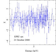
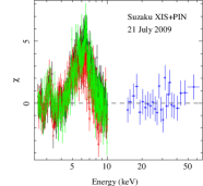
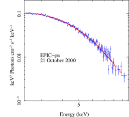
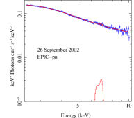
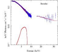
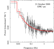
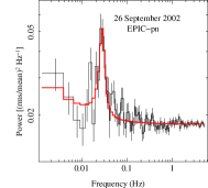
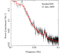
Figure 1: Results of spectral and temporal analysis of Suzaku and XMM-Newton observations of LMC X–1. Top panels: Deviations of the observed XMM-Newton EPIC-pn xmm-101, xmm-401 and Suzaku XIS+PIN spectral data from the best-fitting tbvarabs$\times$(diskbb + simpl) models. Middle panels: Unfolded EPIC-pn xmm-101, xmm-101 and Suzaku XIS+PIN spectral data and the best-fitting models tbvarabs$\times$(diskbb + simpl) for xmm-101 and tbvarabs$\times$(diskbb + simpl + laor) for Suzaku and xmm-401 data. Bottom panels: The power density spectra and the best-fitting models for the xmm-101, xmm-401 and Suzaku/XIS data.

For xmm-401, the absorbed diskbb model resulted in a statistically unacceptable fit ($\chi^{2}/dof=5629.6/156$) due to the presence of a hard component. Use of the Comptonization model simpl (model A) improved the fit ($\chi^{2}/dof=169.4/154$). Careful examination of the fit-residuals showed a hint of broad iron line. We excluded the $5-8{\rm~{}keV}$ band, performed the fitting and compared the observed data with the continuum model. We added the laor line with the emissivity index fixed at $q=3$. The model B improved the fit ($\Delta\chi^{2}=-23.9$ for three parameters). We also calculated $1\sigma$ error on the line flux and found that the broad iron line is detected at a $3.3\sigma$ level. Next we replaced the laor line with reflionx convolved with kdblur (model C) with emissivity index fixed at $q=3$. This model also resulted in a good fit ($\chi^{2}/dof=142.2/151$). The best-fit parameters are listed in Table 2. For the Suzaku and xmm-401 data, the best-fit equivalent Hydrogen column density is in the range of $0.8-1.8\times 10^{22}{\rm~{}cm^{-2}}$ while for the xmm-101 data we could only obtain the $90\%$ upper limit ($N_{H}<0.7\times 10^{22}{\rm~{}cm^{-2}}$). These values are generally consistent with earlier measurements. Using six soft X-ray spectra obtained with grating and/or CCD, Hanke et al. 2010 measured $N_{H}=(1-1.3)\times 10^{22}{\rm~{}cm^{-2}}$ for the diskbb$\ast$simpl model and $N_{H}=(1-2)\times 10^{22}{\rm~{}cm^{-2}}$ for the diskbb$\times$powerlaw model, with a systematic dependence on the orbital phase. Earlier measurements with Chandra, BeppoSAX, ASCA and BBXRT span a range of $4.4-8.6\times 10^{21}{\rm~{}cm^{-2}}$ (see Table 2 in Orosz et al. 2009).

5 Discussion & Conclusions

We have performed power and energy spectral study of the persistent BHB LMC X–1. The PDS shape of LMC X–1 as measured with XMM-Newton and Suzaku is approximately a power-law ($P\propto\nu^{\alpha}$; $\alpha\sim-1$), with rms variability of $4.3\%$ (xmm-101), $2.7\%$ (xmm-401) and $4.2\%$ (Suzaku) in the $10^{-3}-1{\rm~{}Hz}$ range. These values are generally consistent with earlier measurements by Ginga (Ebisawa et al., 1989), RXTE (e.g., Wilms et al., 2001) and typical of a HSS. We have discovered QPOs from LMC X–1 at around $27{\rm~{}mHz}$ in XMM-Newton (xmm-401) and Suzaku observations. These QPOs appear to be remarkable as their centroid frequencies are very low compared to that of A, B or C-type QPOs observed from black hole transients in outburst. Additionally, they appear in the HSS when QPOs are usually not observed. The quality factor of these QPOs ($Q\sim 4$ for xmm-401, $\sim 10$ for Suzaku data) are comparable to that of type B or C QPOs and the rms ($\sim 1.1-1.7\%$) are comparable to type A QPOs. However, the frequencies are much lower than that observed from type A and B QPOs, and the very low frequency type C QPOs are seen only in hard states, much different from what we observe here.

There are very few QPOs from the persistent and wind-fed BHB. In the case of LMC X–1, Ebisawa et al. (1989) claimed detection of QPOs at $75{\rm~{}mHz}$ and $142{\rm~{}mHz}$ with $2.9\%$ and $1.8\%$ rms, respectively, based on Ginga observations. The weaker QPO is likely to be the second harmonic. Thus, the frequencies of the QPOs discovered with Ginga are higher but the $rms$ of these QPOs are within the range of those measured with XMM-Newton and Suzaku observations. It is likely that all these QPOs are similar in nature but vary in their peak frequencies.

The X-ray energy spectrum of LMC X–1 is dominated by two spectral components – accretion disk black body and a Comptonising component or a steep power-law as was also noted earlier (see Ebisawa et al., 1989; Schlegel et al., 1994; Schmidtke et al., 1999; Nowak et al., 2001; Wilms et al., 2001; Gierliński et al., 2001; Ruhlen et al., 2011; Steiner et al., 2012). We have confirmed the broad, relativistic iron line from LMC X–1 in the Suzaku data, earlier studied in detail by Steiner et al. (2012) who measured the black hole spin parameter $a=0.97_{-0.25}^{+0.02}$ ($68\%$ range). We measure the inner radius to be $r_{in}=2.4_{-0.2}^{+0.6}r_{g}$, which corresponds to a similar spin parameter though we used a simpler model. In addition, we also detected broad iron line in one of the XMM-Newton observation (xmm-401). However, the line was narrower ($r_{in}>32r_{g}$) and weaker by at least an order of magnitude compared to the relativistic line measured with the Suzaku data. We did not detect an iron line in the xmm-101 observation. The $90\%$ upper limit on the flux of a laor line at $6.7{\rm~{}keV}$ with $r_{in}=64r_{g}$ (similar to the line in the xmm-401 data) is $3.8\times 10^{-5}{\rm~{}photons~{}cm^{-2}~{}s^{-1}}$. This $90\%$ limit on the iron line flux is nearly two orders of magnitude lower than the line flux measured in the Suzaku data but it is formally consistent with the $90\%$ range measured with the xmm-401 data. In any case, the iron line from LMC X–1 is variable and is only detected clearly when a strong power-law component is present.

We have also found strong variability of the power-law component in the energy spectrum. In the first XMM-Newton observation (xmm-101), the power-law component is almost absent. In this observation, the fraction of the disk emission in the $2-20{\rm~{}keV}$ was $\sim 94\%$ and LMC X–1 was in the soft state. In the second XMM-Newton (xmm-401) and the Suzaku observations, the power-law component was very strong with disk fractions $\sim 35\%$ and $\sim 60\%$, respectively, in the $2-20{\rm~{}keV}$ band (see tab. 2). The spectral variability of LMC X–1 is also well studied. Schmidtke et al. (1999) showed that spectral variability of LMC X–1 mainly arises from the changes in the intensity of the high-energy power-law component.

The clear presence of the broad iron line as well as the QPOs in the X-ray emission from LMC X–1 appear to depend on the presence of a strong power-law component. The QPOs must arise from the inner regions where substantial X-ray variability is produced. Indeed, there are theoretical models that show oscillations in the inner regions of accretion disks. Titarchuk & Osherovich (2000) have shown that the very low frequency QPOs in both BHB and NS XRBs are caused by global disk oscillations in the direction normal to the disk. They argue that these disk oscillations are the result of gravitational interaction between the compact object and the accretion disk. The frequency of the global disk oscillations can be written as

$$\nu_{0}\approx 2\left(\frac{R_{in}}{3R_{S}}\right)^{-\frac{8}{15}}\left(\frac{M_{BH}}{M_{\odot}}\right)^{-\frac{8}{15}}\left(\frac{P_{orb}}{3hr}\right)^{-\frac{7}{15}}\left(\frac{R_{adj}}{R_{in}}\right)^{-0.3}{\rm Hz}$$ (1)

(Titarchuk & Osherovich, 2000). Using $P_{orb}=3.9{\rm~{}days}$, $M_{BH}=10.9M_{\odot}$ (Orosz et al., 2009), $R_{in}=2.3R_{g}$ from the broad iron line fit to the Suzaku data (see Table 2), and the adjustment radius $R_{adj}=2R_{in}$ (Titarchuk & Osherovich, 2000), we find $\nu_{0}\approx 0.15{\rm~{}Hz}$. Thus, the global disk oscillations are $\sim 5$ times faster than the observed QPOs. Hence, the global mode oscillations are unlikely to explain the observed QPOs from LMC X–1.

Very low frequency QPOs in the ${\rm~{}mHz}$ range have been observed from BHBs e.g., the dynamic QPOs in the $1{\rm~{}mHz}-10{\rm~{}Hz}$ range changing their frequency on minutes (Morgan et al., 1997), the “heartbeat” QPOs from GRS 1915+105 (Belloni et al., 2000) and IGR J17091–3624 (Altamirano et al., 2011a). The millihertz heartbeat QPOs from GRS 1915+105 and IGR J17091–3624 occur during the high-luminosity, soft-states and are thought to be due to limit-cycle oscillations of local accretion rate in the inner disk (Neilsen et al., 2011). The millihertz QPOs from LMC X–1 are also detected in the high luminosity ($\sim 0.5L_{Edd}$) with strong soft component. However, the scattering fraction ($f_{SC}\raisebox{-2.15277pt}{$\;\stackrel{{\scriptstyle>}}{{\sim}}\;$}0.13-1$; Neilsen et al. (2011)) of GRS 1915+105 during the heartbeat oscillation appears to be higher than the averaged scattering fraction $f_{SC}\sim 0.1$ we found in the presence of QPO for LMC X–1. Also $rms$ amplitude of the QPOs from LMC X–1 are low ($1-2\%$) compared to the $rms$ amplitude of the hearbeat QPOs from GRS 1915+105, though the amplitude can be as low as $\sim 3\%$ in the case of IGR J17091–3624 (see e.g., Altamirano et al., 2011b). Moreover, the hearbeat oscillations in the $\rho$ and $\mu$ classes of GRS 1915+105 and IGR J17091–3624 generally depict a peculiar pattern – slow rise and fast decay with changes in the count rates by factors $\sim 2-5$ (e.g., Belloni et al., 2000; Altamirano et al., 2011a; Rao & Vadawale, 2012). Though it is difficult to infer the pattern of individual variability events, such large amplitude variability are not seen in the lightcurves of LMC X–1. Thus, the $mhz$ QPOs from LMC X–1 are unlikely to be the “heartbeat” QPOs.

Very low frequency, “non-heartbeat” oscillations have also been found in BHBs. Altamirano & Strohmayer (2012) have reported $11{\rm~{}mHz}$ QPOs from the Black Hole Candidate H 1743–322 in its successive outbursts eight months apart. These QPOs were almost constant in their peak frequency and were detected in the LHS state of H 1743–322. Given the differences in the spectral states and luminosity of LMC X–1 and H 1743–322, it is likely that the QPOs from these two sources arise from different physical phenomena.

The QPOs we detected from LMC X–1 are in the same frequency range as those observed in some ULXs, where there are attempts to identify them in order to scale with mass. If these are the same features, ULXs would host a black hole of a few solar masses. The ${\rm~{}mHz}$ QPOs from LMC X–1 are the only low frequency QPOs from any persistent, wind-fed BHB. A detailed study of the these QPOs and their dependence on energy, broadband energy spectral and PDS shape, absorption will be required to investigate their nature. The variable nature of these QPOs and the broad iron line from LMC X–1 possibly related to strength of the power-law component can be used to study the disk-corona coupling and the origin of both these features. The ASTROSAT mission, scheduled to launch in a year, is well suited for detailed study of these QPOs.

References

- Altamirano et al. (2011a) Altamirano D. et al., 2011a, ApJ, 742, L17
- Altamirano et al. (2011b) Altamirano D. et al., 2011b, The Astronomer’s Telegram, 3225, 1
- Altamirano & Strohmayer (2012) Altamirano D., Strohmayer T., 2012, ApJ, 754, L23
- Belloni & Hasinger (1990) Belloni T., Hasinger G., 1990, A&A, 230, 103
- Belloni et al. (2000) Belloni T., Klein-Wolt M., Méndez M., van der Klis M., van Paradijs J., 2000, A&A, 355, 271
- Belloni et al. (1997) Belloni T., van der Klis M., Lewin W. H. G., van Paradijs J., Dotani T., Mitsuda K., Miyamoto S., 1997, A&A, 322, 857
- Belloni (2010) Belloni T. M., 2010, in Lecture Notes in Physics, Berlin Springer Verlag, Vol. 794, Lecture Notes in Physics, Berlin Springer Verlag, Belloni T., ed., p. 53
- Belloni et al. (2011) Belloni T. M., Motta S. E., Muñoz-Darias T., 2011, Bulletin of the Astronomical Society of India, 39, 409
- Belloni et al. (2012) Belloni T. M., Sanna A., Méndez M., 2012, MNRAS, 426, 1701
- Caballero-García et al. (2013) Caballero-García M. D., Belloni T., Zampieri L., 2013, MNRAS, 436, 3262
- Casella et al. (2004) Casella P., Belloni T., Homan J., Stella L., 2004, A&A, 426, 587
- Casella et al. (2005) Casella P., Belloni T., Stella L., 2005, ApJ, 629, 403
- Corbel et al. (2013) Corbel S., Coriat M., Brocksopp C., Tzioumis A. K., Fender R. P., Tomsick J. A., Buxton M. M., Bailyn C. D., 2013, MNRAS, 428, 2500
- Cowley et al. (1995) Cowley A. P., Schmidtke P. C., Anderson A. L., McGrath T. K., 1995, PASP, 107, 145
- Dewangan et al. (2006) Dewangan G. C., Titarchuk L., Griffiths R. E., 2006, ApJ, 637, L21
- Dheeraj & Strohmayer (2012) Dheeraj P. R., Strohmayer T. E., 2012, ApJ, 753, 139
- Ebisawa et al. (1989) Ebisawa K., Mitsuda K., Inoue H., 1989, PASJ, 41, 519
- Gierliński et al. (2001) Gierliński M., Maciołek-Niedźwiecki A., Ebisawa K., 2001, MNRAS, 325, 1253
- Gou et al. (2009) Gou L. et al., 2009, ApJ, 701, 1076
- Hanke et al. (2010) Hanke M., Wilms J., Nowak M. A., Barragán L., Schulz N. S., 2010, A&A, 509, L8
- Lewin & van der Klis (2006) Lewin W. H. G., van der Klis M., 2006, Compact Stellar X-ray Sources
- Markwardt et al. (1999) Markwardt C. B., Swank J. H., Taam R. E., 1999, ApJ, 513, L37
- Miller (2007) Miller J. M., 2007, ARAA, 45, 441
- Morgan et al. (1997) Morgan E. H., Remillard R. A., Greiner J., 1997, ApJ, 482, 993
- Motta et al. (2009) Motta S., Belloni T., Homan J., 2009, MNRAS, 400, 1603
- Motta et al. (2011) Motta S., Muñoz-Darias T., Casella P., Belloni T., Homan J., 2011, MNRAS, 418, 2292
- Mucciarelli et al. (2006) Mucciarelli P., Casella P., Belloni T., Zampieri L., Ranalli P., 2006, MNRAS, 365, 1123
- Neilsen et al. (2011) Neilsen J., Remillard R. A., Lee J. C., 2011, ApJ, 737, 69
- Nowak et al. (2001) Nowak M. A., Wilms J., Heindl W. A., Pottschmidt K., Dove J. B., Begelman M. C., 2001, MNRAS, 320, 316
- Orosz et al. (2009) Orosz J. A. et al., 2009, ApJ, 697, 573
- Pasham & Strohmayer (2013) Pasham D. R., Strohmayer T. E., 2013, ApJ, 771, 101
- Rao & Vadawale (2012) Rao A., Vadawale S. V., 2012, ApJ, 757, L12
- Remillard & McClintock (2006) Remillard R. A., McClintock J. E., 2006, ARAA, 44, 49
- Remillard et al. (1999) Remillard R. A., Morgan E. H., McClintock J. E., Bailyn C. D., Orosz J. A., 1999, ApJ, 522, 397
- Reynolds & Nowak (2003) Reynolds C. S., Nowak M. A., 2003, PhR, 377, 389
- Ross & Fabian (2005) Ross R. R., Fabian A. C., 2005, MNRAS, 358, 211
- Ross et al. (1999) Ross R. R., Fabian A. C., Young A. J., 1999, MNRAS, 306, 461
- Ruhlen et al. (2011) Ruhlen L., Smith D. M., Swank J. H., 2011, ApJ, 742, 75
- Schlegel et al. (1994) Schlegel E. M., Marshall F. E., Mushotzky R. F., Smale A. P., Weaver K. A., Serlemitsos P. J., Petre R., Jahoda K. M., 1994, ApJ, 422, 243
- Schmidtke et al. (1999) Schmidtke P. C., Ponder A. L., Cowley A. P., 1999, aj, 117, 1292
- Steiner et al. (2009) Steiner J. F., Narayan R., McClintock J. E., Ebisawa K., 2009, PASP, 121, 1279
- Steiner et al. (2012) Steiner J. F. et al., 2012, MNRAS, 427, 2552
- Strohmayer & Mushotzky (2003) Strohmayer T. E., Mushotzky R. F., 2003, ApJ, 586, L61