A light NMSSM pseudoscalar Higgs boson at the LHC redux

Abstract

The Next-to-Minimal Supersymmetric Standard Model (NMSSM) contains a singlet-like pseudoscalar Higgs boson in addition to the doublet-like pseudoscalar of the Minimal Supersymmetric Standard Model. This new pseudoscalar can have a very low mass without violating the LEP exclusion constraints and it can potentially provide a hallmark signature of non-minimal supersymmetry at the LHC. In this analysis we revisit the light pseudoscalar in the NMSSM with partial universality at some high unification scale. We delineate the regions of the model’s parameter space that are consistent with the up-to-date theoretical and experimental constraints, from both Higgs boson searches and elsewhere (most notably $b$-physics), and examine to what extent they can be probed by the LHC. To this end we review the most important production channels of such a Higgs state and assess the scope of its observation at the forthcoming Run-2 of the LHC. We conclude that the $b\bar{b}$-associated production of the pseudoscalar, which has been emphasised in previous studies, does not carry much promise anymore, given the measured mass of the Higgs boson at the LHC. However, the decays of one of the heavier scalar Higgs bosons of the NMSSM can potentially lead to the discovery of its light pseudoscalar. Especially promising are the decays of one or both of the two lightest scalar states into a pseudoscalar pair and of the heaviest scalar into a pseudoscalar and a $Z$ boson. Since the latter channel has not been explored in detail in the literature so far, we provide details of some benchmark points which can be probed for establishing its signature.

1 Introduction

The Next-to-Minimal Supersymmetric Standard Model (NMSSM)Fayet:1974pd ; Ellis:1988er ; Durand:1988rg ; Drees:1988fc ; Miller:2003ay contains a singlet Higgs field in addition to the two doublet fields of the Minimal Supersymmetric Standard Model (MSSM). This results in two additional neutral mass eigenstates, one scalar and one pseudoscalar, in the Higgs sector, on top of the three MSSM-like ones. Naturally, these new Higgs bosons are singlet-dominated, implying that their couplings to the fermions and gauge bosons of the Standard Model (SM) are typically much smaller than those of the doublet-dominated Higgs bosons. Their masses are thus generally very weakly constrained by the Higgs boson data from the Large Electron Positron (LEP) collider as well as the Large Hadron Collider (LHC), and can be as low as a few $\,\mathrm{GeV}$. Evidently, the observation of any of these potentially light states, in addition to the SM-like Higgs boson discovered alreadyAad:2012tfa ; Chatrchyan:2012ufa , will provide a clear indication of not just physics beyond the SM but also of a non-minimal nature of supersymmetry (SUSY).

In particular, the lightest NMSSM pseudoscalar, $A_{1}$, is a crucial probe of new physics as it can be tested at the already established searches for a supersymmetric pseudoscalar Higgs boson performed by many experimental groupsLove:2008aa ; Tung:2008gd ; Lees:2012iw ; Lees:2012te ; Lees:2013vuj ; Peruzzi:2014ksa . These searches are sensitive only to very light pseudoscalars Higgs bosons which could result from the decays of heavy mesons. The results from the CLEO experimentLove:2008aa have in fact been used in the past to directly constrain the mass of the NMSSM $A_{1}$Domingo:2008rr . Heavier, $\gtrsim 5$$\,\mathrm{GeV}$, pseudoscalars have also been probed in the possible decay of a heavy SM-like scalar Higgs boson at LEP2Schael:2010aw . More recently, the LHC has searched for a light pseudoscalar decaying in the $\mu^{+}\mu^{-}$ channel and produced either singly in $pp$ collisionsChatrchyan:2012am or in pairs from the decays of a non-SM-like Higgs bosonChatrchyan:2012cg .

In the context of the NMSSM, the production of $A_{1}$ via decays of other heavy Higgs bosons has been the subject of a number of studiesEllwanger:2003jt ; Ellwanger:2005uu ; Moretti:2006hq ; Forshaw:2007ra ; Belyaev:2008gj ; Almarashi:2011te , aiming at establishing a “no-lose” theorem for the discovery of the NMSSM Higgs bosons (seeEllwanger:2013ova for a recent review). Other possible production processes have also been investigated in the literature. InCheung:2008rh the production of a light $A_{1}$ in association with a light neutralino via the decay of heavier neutralinos was discussed. $b\bar{b}$-associated production of the NMSSM $A_{1}$ at the LHC followed by decays in the $\tau^{+}\tau^{-}$ and the $\mu^{+}\mu^{-}$ channels was studied inAlmarashi:2010jm ; Almarashi:2011hj , respectively. Assuming the same production process, it was established inAlmarashi:2011bf that an $A_{1}$, with $20\,\mathrm{GeV}\lesssim m_{A_{1}}\lesssim 80$$\,\mathrm{GeV}$, could be observed with very large luminosity at the LHC in the $b\bar{b}$ decay channel. This is made possible by an enhanced coupling of $A_{1}$ to $b\bar{b}$ pairs for certain configurations of the model parametersAlmarashi:2012ri . $b\bar{b}$-associated production also affords the possibility to search for the $H_{\rm SM}\rightarrow A_{1}Z$ decay modeAlmarashi:2011qq , where $H_{\rm SM}$ is our notation for the generic SM-like Higgs boson of the model. We should point out here that in the NMSSM both $H_{1}$ and $H_{2}$, the lightest and next-to-lightest CP-even Higgs bosons, respectively, can alternatively play the role of $H_{\rm SM}$Ellwanger:2011aa ; King:2012is ; Ellwanger:2012ke ; Gherghetta:2012gb ; Cao:2012fz .

All the above mentioned analyses were, however, performed prior to the discovery of the Higgs boson at the LHCChatrchyan:2012ufa ; Aad:2012tfa . Thenceforth, inKim:2012az the $A_{1}\rightarrow\gamma\gamma$ decay channel was studied for a light $A_{1}$. InMunir:2013wka it was noted that in the NMSSM the $A_{1}$ could in fact be degenerate in mass with the SM-like Higgs boson. It could thus cause an enhancement in the Higgs boson signal rates near 125 $\,\mathrm{GeV}$ in the $\gamma\gamma$, $b\bar{b}$ and $\tau^{+}\tau^{-}$ channels simultaneously provided, again, that it is produced in association with a $b\bar{b}$ pair. InCerdeno:2013cz the $H_{\rm SM}\rightarrow A_{1}A_{1}\rightarrow 4\ell$ (with $\ell$ denoting $e^{\pm}$ and $\mu^{\pm}$) process at the LHC has been studied in detail. The production of $A_{1}$ via neutralino decays has also been recently revisited inStal:2011cz ; Das:2012rr ; Cerdeno:2013qta . Finally, NMSSM benchmark proposals capturing much of this phenomenology also existDjouadi:2008uw ; King:2012tr ; Curtin:2013fra ; King:2014xwa . In this article we analyse in detail some of the production processes that yield a sizeable cross section and could potentially lead to the detection of a light NMSSM $A_{1}$ at the LHC with $\sqrt{s}=14$$\,\mathrm{TeV}$. We perform parameter scans of the NMSSM with partial universality at the Grand Unification Theory (GUT) scale to find regions where a light, $\lesssim 150$$\,\mathrm{GeV}$, $A_{1}$ can be obtained. In these scans we require the mass of $H_{\rm SM}$ to lie around 125$\,\mathrm{GeV}$ and its signal rates in the $\gamma\gamma$ and $ZZ$ channels to be consistent with the SM expectations. We study in detail the two possibilities, ${H_{\rm SM}}=H_{1}$ and ${H_{\rm SM}}=H_{2}$, as two separate cases. Moreover, we divide the production mode of the $A_{1}$ into two main categories: 1) direct production in association with a $b\bar{b}$ pair, which we refer to as the $bbA_{1}$ mode in the following, and 2) via decay of a heavy scalar Higgs boson of the model.

In the second category mentioned above, we include the two main production channels of the pseudoscalar, namely $A_{1}A_{1}$ and $A_{1}Z$. Furthermore, the decaying heavier Higgs boson can be any of the three neutral scalars, $H_{1}$, $H_{2}$ and $H_{3}$. $A_{1}$’s thus produced decay into either $b\bar{b}$ or $\tau^{+}\tau^{-}$ pairs. The former decay channel is always the dominant one as the ratio of the Branching Ratios (BRs) for these channels is given approximately by the ratio of the $b$ and $\tau$ masses, but the latter can be equally important due to a relatively small $\tau^{+}\tau^{-}$ background. In case of the $A_{1}Z$ decay channel, we only consider the leptonic ($e^{+}e^{-}$ and $\mu^{+}\mu^{-}$) decays of the $Z$ boson. To study the prospects for the discovery of an $A_{1}$ at the LHC in all these production and decay channels, we employ hadron level Monte Carlo (MC) simulations. We perform a detailed signal-to-background analysis for each process of interest, employing a jet substructure method for detecting the $b$ quarks originating from an $A_{1}$ decay.

The article is organised as follows. In section 2, we will briefly discuss the model under consideration and some important properties of the singlet-like pseudoscalar in it. In section 3 we will explain our methodology for NMSSM parameter space scans as well as for our signal-to-background analyses of the $A_{1}$ production and decay processes considered. In section 4 we will discuss our results in detail. Finally, we will present our conclusions in section 5.

2 The light pseudoscalar $A_{1}$ in the NMSSM

The scale-invariant superpotential of the NMSSM (see, e.g.,Ellwanger:2009dp ; Maniatis:2009re for reviews) is defined in terms of the two NMSSM Higgs doublet superfields $\widehat{H}_{u}$ and $\widehat{H}_{d}$ along with an additional Higgs singlet superfield $\widehat{S}$ as

$$W_{\rm NMSSM}\ =\ {\rm MSSM\;Yukawa\;terms}\>+\>\lambda\widehat{S}\widehat{H}_{u}\widehat{H}_{d}\>+\>\frac{\kappa}{3}\ \widehat{S}^{3}\,,$$ (1)

where ${\lambda}$ and ${\kappa}$ are dimensionless Yukawa couplings. Upon spontaneous symmetry breaking, the superfield $\widehat{S}$ develops a vacuum expectation value (VEV), $s\equiv\langle\widehat{S}\rangle$, generating an effective $\mu$-term, $\mu_{\rm{eff}}={\lambda}s$. The soft SUSY-breaking terms in the scalar Higgs sector are then given by

$$V_{\rm{soft}}=m_{H_{u}}^{2}|H_{u}|^{2}+m_{H_{d}}^{2}|H_{d}|^{2}+m_{S}^{2}|S|^{2}+\left({\lambda}{A_{\lambda}}SH_{u}H_{d}+\frac{1}{3}{\kappa}{A_{\kappa}}S^{3}+\textrm{h.c.}\right)\,.$$ (2)

Due to the presence of the additional singlet field, the NMSSM contains several new parameters besides the 150 or so parameters of the MSSM. However, assuming the sfermion mass matrices and the scalar trilinear coupling matrices to be diagonal reduces the parameter space of the model considerably. One can further impose universality conditions on the dimensionful parameters at the GUT scale, leading to the so-called Constrained NMSSM (CNMSSM). Thus all the scalar soft SUSY-breaking masses in the superpotential are unified into a generic mass parameter ${m_{0}}$, the gaugino masses into $m_{1/2}$, and all the trilinear couplings, including ${A_{\lambda}}$^∗ and ${A_{\kappa}}$^∗ (defined at the GUT scale), into $A_{0}$. Then, given that the correct $Z$ boson mass, $m_{Z}$, is known, ${m_{0}}$, $m_{1/2}$, $A_{0}$, the coupling ${\lambda}$, taken as an input at the SUSY-breaking scale, $M_{\rm SUSY}$, and the sign of $\mu_{\rm{eff}}$ constitute the only free parameters of the CNMSSM.

As noted inKowalska:2012gs , the fully constrained NMSSM struggles to achieve the correct mass for the assumed SM-like Higgs boson, particularly in the presence of other important experimental constraints. Furthermore, the parameters governing the mass of the singlet-like pseudoscalar Higgs boson, which will be discussed below, are not input parameters themselves, but are calculated at the electroweak (EW) scale starting from the four GUT-scale parameters. In order to avoid these issues the unification conditions noted above need to be relaxed. In a partially unconstrained version of the model the soft masses of the Higgs fields, $m_{H_{u}}$, $m_{H_{d}}$ and $m_{S}$, are disunified from ${m_{0}}$ and taken as free parameters at the GUT scale. Through the minimisation conditions of the Higgs potential these three soft masses can then be traded at the EW scale for the parameters ${\kappa}$, $\mu_{\rm{eff}}$ and $\tan\beta$. Similarly, the soft trilinear coupling parameters ${A_{\lambda}}$^∗ and ${A_{\kappa}}$^∗, though still input at the GUT scale, are disunified from $A_{0}$. The model is thus defined in terms of the following nine continuous input parameters:

${m_{0}}$, $m_{1/2}$, $A_{0}$, $\tan\beta$, ${\lambda}$, ${\kappa}$, $\mu_{\rm{eff}}$, ${A_{\lambda}}$^∗, ${A_{\kappa}}$^∗,

where $\tan\beta\equiv v_{u}/v_{d}$, with $v_{u}$ being the VEV of the $u$-type Higgs doublet and $v_{d}$ that of the $d$-type one. This version of the model serves as a good approximation of the most general EW-scale NMSSM as far as the phenomenology of the Higgs sector is concerned. In this way, one can minimise the number of free parameters in a physically motivated way instead of imposing any ad-hoc conditions, as would be needed for the general NMSSM. We, therefore, adopt this model to analyse the phenomenology of the light pseudoscalar here. We refer to it as the CNMSSM-NUHM, where NUHM stands for non-universal (soft) Higgs masses, in the following.

2.1 Mass of $A_{1}$

The presence of an extra singlet Higgs field in the NMSSM results in a total of five neutral Higgs mass eigenstates, scalars $H_{1,2,3}$ and pseudoscalars $A_{1,2}$, and a charged pair $H^{\pm}$, after rotating away the Goldstone bosons. The tree-level mass of $A_{1}$ can be given by the approximate expression

$$m_{A_{1}}^{2}\simeq{\lambda}({A_{\lambda}}+4{\kappa}s)\frac{v^{2}\sin 2\beta}{2s}-3\kappa sA_{\kappa}-\frac{M^{4}_{P,12}}{M^{2}_{P,11}}$$ (3)

where $v\equiv\sqrt{v_{u}^{2}+v_{d}^{2}}\simeq 174$$\,\mathrm{GeV}$ and all the parameters are defined at $M_{\rm SUSY}$. $M^{2}_{P,12}$ and $M^{2}_{P,11}$ in the above equation correspond to the off-diagonal and the doublet-like diagonal elements, respectively, of the symmetric $2\times 2$ pseudoscalar mass matrix. Note that since $m_{A_{1}}^{2}$ is proportional to ${\lambda}\sin 2\beta$, the effect of an increase in ${\lambda}$ with fixed $\tan\beta$ is analogous to that of a decrease in $\tan\beta$ with fixed ${\lambda}$. Thus, in the following, whenever the dependence of $m^{2}_{A_{1}}$ on ${\lambda}$ is analysed, the inverse dependence on $\tan\beta$ is implicit. Assuming negligible singlet-doublet mixing, one can ignore the third term on the right hand side of eq. (3) and rewrite it as

$$m_{A_{1}}^{2}\simeq\frac{{A_{\lambda}}}{2s}v^{2}{\lambda}\sin 2\beta+{\kappa}(2v^{2}{\lambda}\sin 2\beta-3s{A_{\kappa}})\,.$$ (4)

Then, for given signs and absolute values of ${A_{\lambda}}$ and ${A_{\kappa}}$, the mass of $A_{1}$ depends on the sizes of ${\lambda}$ and ${\kappa}$ (which are both taken to be positive here along with $\mu_{\rm{eff}}$, and hence $s$). This leads to four possible scenarios, as explained below.

${A_{\kappa}}<0$. The second term on the right hand side of eq. (4) is positive. In this case one has the following.

• ${A_{\lambda}}>0$ leads to a positive first term also. $m^{2}_{A_{1}}$ increases with increasing ${\lambda}$ and/or ${\kappa}$.

• ${A_{\lambda}}<0$ gives a negative first term. Increasing ${\lambda}$ increases the size of this term as well as of the positive second term. Thus, in order to avoid an overall negative $m_{A_{1}}^{2}$, ${\kappa}$ ought to be large enough so that the second term dominates over the negative first term. $m_{A_{1}}^{2}$ then increases further with increasing ${\kappa}$, while the size of ${\lambda}$ is much less significant.

${A_{\kappa}}>0$. In this case one has the following.

• $|2{\lambda}\ v^{2}\sin 2\beta|>|3s{A_{\kappa}}|$ implies a positive second term. The dependence of $m_{A_{1}}^{2}$ on ${A_{\lambda}}$, ${\lambda}$ and ${\kappa}$ is similar to the ${A_{\kappa}}<0$ case above.

• $|2{\lambda}\ v^{2}\sin 2\beta|<|3s{A_{\kappa}}|$ results in a negative second term. For ${A_{\lambda}}>0$ the first term is positive and can dominate over the second term for small enough ${\kappa}$. Decreasing ${\kappa}$ thus increases $m_{A}^{2}$, almost irrespectively of the size of ${\lambda}$. ${A_{\lambda}}<0$ is not allowed as it results in $m_{A}^{2}<0$ owing to a negative first term also.

2.2 Production of $A_{1}$

At the LHC, $A_{1}$ can either be produced directly in the conventional Higgs boson production modes or, alternatively, through decays of the other Higgs bosons of the NMSSM. We study in detail both of these possibilities. The $A_{1}$ thus produced can then decay via a long list of available channels, out of which only the final states with $b$ and $\tau$ pairs are of numerical relevance.

Direct production.  As noted earlier, the $gg\rightarrow bbA_{1}$ channel is the preferred direct mode of producing $A_{1}$ at the LHC, owing to the possibility of a considerably enhanced $b\bar{b}A_{1}$ coupling compared to the $ggA_{1}$ effective coupling in the NMSSM. We refer the reader toMunir:2013wka for details of the parameter configurations that can yield such an enhancement. Here we shall discuss the detectability of a light, $\lesssim 150$$\,\mathrm{GeV}$, $A_{1}$ produced in this mode at the LHC.

Indirect production.  We refer to the processes covered by this production category generically as $H^{\prime\prime}\rightarrow A_{1}A_{1}/Z$, and consider only the gluon fusion (GF) channel for the production of the parent Higgs boson, $H^{\prime\prime}$, at the LHC. There are two further distinct possibilities regarding $H^{\prime\prime}$ for a given model point. It can either be $H_{\rm SM}$, in which case its mass measurement from the LHC serves as an additional kinematical handle. Alternatively, the parent Higgs boson can be one of the other two CP-even states, which we denote collectively by $H^{\prime}$. This kind of processes are particularly important for $m_{A_{1}}>m_{H_{\rm SM}}/2$, although removing the condition on the final states to have a combined invariant mass close to 125$\,\mathrm{GeV}$ reduces the experimental sensitivity by a factor of $2$ to $3$.

For $m_{A_{1}}<m_{H^{\prime\prime}}-m_{Z}$ both $H^{\prime\prime}\to A_{1}Z$ and $H^{\prime\prime}\to A_{1}A_{1}$ processes can be accessible. For the $A_{1}Z$ channel we only take the $Z\rightarrow\ell^{+}\ell^{-}$ decay into account, where $\ell^{+}\ell^{-}$ ($2\ell$) stands for $\mu^{+}\mu^{-}$ and $e^{+}e^{-}$ combined (due to the ease of their detection we do not separate these two final states). This is because the experimental sensitivity for these states is much better than that for the $\tau^{+}\tau^{-}$ and $q\bar{q}$ pairs. We ignore the $H^{\prime\prime}\rightarrow A_{1}Z^{*}$ decay, i.e., with the $Z$ boson off mass shell. The reason is that the width of the $H^{\prime\prime}\rightarrow A_{1}Z$ decay process is already very small when it is allowed kinematically and becomes almost negligible for an off-shell $Z$. Thus, for $m_{A_{1}}>m_{H^{\prime\prime}}-m_{Z}$ only the $H^{\prime\prime}\to A_{1}A$ decay channel can be exploited (as long as $m_{A_{1}}<m_{H^{\prime\prime}}/2$). For this channel we consider the $b\bar{b}b\bar{b}$ (4$b$), $b\bar{b}\tau^{+}\tau^{-}$ (2$b$2$\tau$) and $\tau^{+}\tau^{-}\tau^{+}\tau^{-}$ (4$\tau$) final state combinations.

3 Methodology

We performed several scans of the NMSSM parameter space to search for regions yielding $m_{A_{1}}\lesssim 150$$\,\mathrm{GeV}$, using the nested sampling package MultiNest-v2.18Feroz:2008xx . We used the public package NMSSMTools-v4.2.1NMSSMTools for computing the SUSY mass spectrum and BRs of the Higgs bosons for each model point. In our scans, we also required either $H_{1}$ or $H_{2}$ to have a mass near 125$\,\mathrm{GeV}$ and SM-like signal rates. The signal rate, $R_{X}$, for a given decay channel $X$, is defined as

$$R_{X}\equiv\frac{\sigma(gg\rightarrow H_{i})\times{\rm BR}(H_{i}\rightarrow X)}{\sigma(gg\rightarrow h_{\rm SM})\times{\rm BR}(h_{\rm SM}\rightarrow X)}\,,$$ (5)

where ${h_{\rm SM}}$ denotes the SM Higgs boson with a mass equal to that of $H_{i}$, the NMSSM Higgs boson under consideration. Since GF is by far the dominant Higgs boson production mode at the LHC, $R_{X}$ serves as a good approximation for the inclusive theoretical counterpart of the experimentally measured signal strength, $\mu_{X}$, defined as

$$\mu_{X}=\frac{\sigma(pp\rightarrow H_{i}\rightarrow X)}{\sigma(pp\rightarrow h_{\rm SM}\rightarrow X)}\,.$$ (6)

The program NMSSMTools provides the values of $R_{X}$ for the dominant decay channels of each NMSSM Higgs boson as an output for a given model point. It is calculated in terms of the reduced couplings of a NMSSM Higgs boson to various particle pairs, i.e., couplings normalised to the corresponding ones of a SM Higgs boson. However, since the $WW$ and $ZZ$ decays of each $H_{i}$ in the NMSSM depend on the same $VVH_{i}$ reduced coupling, NMSSMTools computes a unique value of the signal rate, $R_{VV}$, for both these channels. But note that, at the LHC, the $\gamma\gamma$ and $ZZ$ decay channels remain the only ones so far where the observed significance of the signal exceeds the expected one, with the latest measurements of the signal strengths in these channels being

$$\mu_{\gamma\gamma}=1.13\pm 0.24\,,\leavevmode\nobreak\ \leavevmode\nobreak\ \leavevmode\nobreak\ \mu_{ZZ}=1.0\pm 0.29\,,$$ (7)

according to the CMS analysesCMS-PAS-HIG-14-009 , and

$$\mu_{\gamma\gamma}=1.57^{+0.33}_{-0.28}\,,\leavevmode\nobreak\ \leavevmode\nobreak\ \leavevmode\nobreak\ \mu_{ZZ}=1.44^{+0.40}_{-0.35}\,,$$ (8)

in the ATLAS analysesATLAS-CONF-2014-009 . We therefore identify the calculated $R_{VV}$ with the signal rate for the $ZZ$ channel and ignore the experimental result for the $WW$ channel.

In our final analysis of the $A_{1}$ production and decay channels at the LHC, for $H_{SM}$ to be consistent with the ATLAS Higgs boson data, its $R_{\gamma\gamma/ZZ}$ is required to lie within the range given in eqs. (8). Similarly, for consistency with the CMS data, $R_{\gamma\gamma/ZZ}$ for $H_{\rm SM}$ should satisfy eqs. (7). Note that these two requirements are imposed separately, since the measurements from the two experiments are not mutually very consistent in all cases and can also be expected to fluctuate somewhat at the next LHC run. It is for this reason that among the ‘good points’ from our scans we will retain also those that do not comply with these robust requirements. All these good points are, however, required to be consistent with the LEP and LHC exclusion limits, applicable on the other, non-SM-like, Higgs bosons of the model and tested using HiggsBounds-v4.1.3Bechtle:2008jh ; Bechtle:2011sb ; Bechtle:2013gu ; Bechtle:2013wla .

The output files of NMSSMTools contain a SLHA Block as input for the HiggsBounds package, which is essentially composed of the squared reduced couplings of all $H_{i}$’s. Here an ambiguity arises due to the fact that HiggsBounds uses these reduced couplings for calculating the cross section ratios (similarly to eq. (5) and its equivalents for other Higgs boson production modes also) for imposing the exclusion limits on the $H_{i}$’s. The $ggH_{i}$ reduced couplings are assumed to take care of also the EW correctionsDjouadi:1994ge ; Degrassi:2004mx ; Actis:2008ug , since HiggsBounds effectively obtains the approximate partonic cross section $\sigma(gg\rightarrow H_{i})$ by multiplying $ggH_{i}$ with the SM counterpart, $\sigma(gg\rightarrow h_{\rm SM})$, evaluated including the EW correctionsDittmaier:2011ti . However, these corrections are not available in the NMSSM and hence are not implemented in NMSSMTools, which only includes the next-to-leading order (NLO) QCD contributions to the $ggH_{i}$ reduced coupling. Since the EW corrections reach only up to 8% with respect to the leading order (LO) cross section and the non-SM-like Higgs bosons generally have very poor signal rates, we ignore this slight ambiguity in the implementation of the collider exclusion limits on them.

During our scans, while the experimental constraints specific to the Higgs sector implemented in NMSSMTools were retained, all the other phenomenological constraints were ignored. Instead, the $b$-physics observables were calculated explicitly for each point using the dedicated package SuperIso-v3.3superiso , for improved theoretical precision. The good points to be shown in our results are also consistent with the following $b$-physics constraints, based onBeringer:1900zz :

• $\rm BR\left(B_{s}\to\mu^{+}\mu^{-}\right)=(3.2\pm 1.35\pm 0.32)\times 10^{-9}$, where the last quantity implies a 10% theoretical error in the numerical evaluation,

• $\rm BR\left(B_{u}\rightarrow\tau\nu\right)=(1.66\pm 0.66\pm 0.38)\times 10^{-4}$,

• $\rm BR\left(\overline{B}\rightarrow X_{s}\gamma\right)=(3.43\pm 0.22\pm 0.21)\times 10^{-4}$.

In addition, these points also satisfy the Dark Matter relic density constraint, $\Omega_{\chi}h^{2}<0.131$, assuming a $+10$% theoretical error around the central value of 0.119 measured by the PLANCK telescopeAde:2013zuv . For calculating the theoretical model prediction for $\Omega_{\chi}h^{2}$ we used the public package MicrOMEGAs-v2.4.5micromegas . Finally, the program NMSSMTools by default discards a SUSY point if the perturbativity constraint is violated or if the global minimum is not a physical one.

3.1 Event analysis

For each process of interest we carry out a dedicated signal-to-background analysis based on MC event generation for proton-proton collisions at 14 TeV centre-of-mass energy. The backgrounds for all the processes are computed with MadGraph5_aMC$@$NLOAlwall:2014hca using its default factorisation and renormalisation scale and the CTEQ6L1cteq6 library for parton distribution functions. The signal cross sections for the GF and $bbh_{\rm SM}$ production modes are computed using SusHi-v1.1.1Harlander:2012pb for the SM Higgs boson. These cross sections are then rescaled using the reduced $bbA_{1}$ and $ggH_{i}$ couplings in the NMSSM and multiplied by the relevant BRs of $H_{i}$, all of which are obtained from NMSSMTools.

These GF cross section obtained from SusHi contains the QCD contributions up to the next-to-next-to-leading order (NNLO)Djouadi:1991tka ; Dawson:1990zj ; Spira:1995rr ; Harlander:2002wh ; Anastasiou:2002yz ; Ravindran:2003um ; Marzani:2008az ; Harlander:2009mq ; Pak:2009dg . However, we make sure to turn off the EW corrections since these are not included in the $ggH_{i}$ reduced couplings obtained from NMSSMTools, which is evaluated taking only the NLO QCD effects into account, as pointed out earlier. In the case of the $bbh_{\rm SM}$ production, note that SusHi calculates only the inclusive $b\bar{b}\to h_{\rm SM}$ cross section at the NNLO in QCDMaltoni:2003pn ; Harlander:2003ai and not the fully exclusive $gg\to b\bar{b}h_{\rm SM}$ process. However, these two cross sections have been found to show reasonable numerical agreement when including higher order correctionsDittmaier:2003ej ; Liu:2012qu . To our advantage, the $b\bar{b}\to h_{\rm SM}$ cross section can be conveniently rescaled with the $bbA_{1}$ reduced coupling obtained from NMSSMTools. Such a rescaling would not be straightforward in the case of the $gg\to b\bar{b}h_{\rm SM}$ process at NLO, due to diagrams with top loops.

Both the signal and the background for each process are hadronised and fragmented using Pythia 8.180Sjostrand:2007gs interfaced with FastJet-v3.0.6Cacciari:2011ma for jet clustering and jet substructure analysis. The parton-level acceptance cuts used in the event generation in MadGraph are

• $|\eta|<$ 2.5 for all final state objects,

• $p_{T}>15$$\,\mathrm{GeV}$ far all final state objects,

• $\Delta R\equiv\sqrt{(\Delta\eta)^{2}+(\Delta\phi)^{2}}>0.2$ for all $b$-quark pairs,

• $\Delta R>0.4$ for all other pairs of final state objects,

where $p_{T}$, $\eta$, $\phi$ are the transverse momentum, pseudorapidity and azimuthal angle, respectively. The looser cut on $\Delta R$ for $b$-quark pairs is to allow the use of the jet substructure method in the later analyses. In table 1 we show the background cross sections after the acceptance cuts have been applied at the parton level. Since the signal events are generated directly in Pythia, the above acceptance cuts are implemented not at the parton level but at the hadron level after jet clustering. For this reason we do not provide any exact efficiency values for the signal processes. However, in general, from around 0.05% for $b\bar{b}Z$ and 10% for $b\bar{b}b\bar{b}$, to almost 100% of the signal events meet the acceptance requirements at the parton level, depending on the masses involved.

Channel	Background cross section
$b\bar{b}b\bar{b}$	3400 pb
$b\bar{b}\tau^{+}\tau^{-}$	3.1 pb
$\tau^{+}\tau^{-}\tau^{+}\tau^{-}$	5.4 fb
$b\bar{b}Z$	126 pb
$\tau^{+}\tau^{-}Z$	0.46 pb

Table 1: Parton-level cross sections for the various backgrounds after applying acceptance cuts, as given by MadGraph.

We do not perform any proper $b$- or $\tau$-tagging but use the MC truth to identify jets that stem from $B$-mesons and $\tau$-leptons, respectively. The single tagging efficiency, 50% for both $b$- and $\tau$-jets, is then taken into account by a scaling of the cross sections, assuming no knowledge of the charge-sign of the jet. Note also that, although we do not include any detector effects or smearing, the hadronisation and consequent jet clustering have a similar effect of broadening the studied objects. We therefore expect the inclusion of smearing due to the detector resolution to only marginally change our results.

In case of the $\tau$-jets in the final state, we use only their visible parts to represent the $\tau$’s. However, we note here that the use of more sophisticated tools for this purpose (see, e.g.,Elagin:2010aw ; Gripaios:2012th ; Bianchini:2014vza ), may help improve the $\tau$-reconstruction efficiency further. When there are only two $\tau$-jets in the final state, one could employ, e.g., the collinear approximationEllis:1987xu to improve the mass resolution. However, in our case the $\tau$’s tend to be too back-to-back for this to work properly.

To identify the $A_{1}$ bosons decaying to $b\bar{b}$ pairs over the QCD background, we employ the jet substructure method ofButterworth:2008iy , used recently indeLima:2014dta to demonstrate the detectability of pair-produced $h_{\rm SM}$ in the $4b$ final state. In this method, we first cluster all final state visible particles using the Cambridge-Aachen (CA) algorithmCambridge ; Aachen with $R=1.2$. For each resulting jet, $j$, that has $p_{T}>30$$\,\mathrm{GeV}$ and an invariant mass $>12$$\,\mathrm{GeV}$, we go back in the clustering sequence until we find two subjets, $j_{1}$ and $j_{2}$, with relatively similar respective invariant masses, $m_{j_{1}}$ and $m_{j_{2}}$, and transverse momenta, $p_{Tj_{1}}$ and $p_{Tj_{2}}$. Furthermore, both $m_{j_{1}}$ and $m_{j_{2}}$ should be significantly lower than the invariant mass, $m_{j}$, of the jet they would subsequently merge into (i.e., the declustered jet $j$). Technically this means that the two subjets are required to satisfy the conditions

$$m_{j_{1,2}}/m_{j}<0.67\leavevmode\nobreak\ \leavevmode\nobreak\ \leavevmode\nobreak\ {\rm and}\leavevmode\nobreak\ \leavevmode\nobreak\ \leavevmode\nobreak\ \frac{\min(p_{Tj_{1}}^{2},p_{Tj_{2}}^{2})}{m_{j}^{2}}\Delta R^{2}(j_{1},j_{2})>0.09\,.$$ (9)

These two subjets are then taken to be potentially coming from an $A_{1}$ and their constituents are reclustered with the CA algorithm with $R=\max(\min(\Delta R(j_{1},j_{2})/2,0.3),0.2)$. If the two hardest of the jets thus obtained are $b$-tagged and the three hardest jets together have an invariant mass $>12$ GeV, the combination of these three subjets is considered a fat jet resulting from the $A_{1}\rightarrow b\bar{b}$ decay. The constituents of the fat jet are then removed from the event and the remaining particles are reclustered using the antikTantikT algorithm with $R=0.4$ in order to find single $b$- and other jets.

We now have three possible signatures for a decaying $A_{1}$: one fat jet, two single $b$-jets and two $\tau$-jets. For the $H^{\prime\prime}\rightarrow A_{1}A_{1}$ decay, one then has six possible combinations to look for. In all cases we require that the difference between the invariant masses of the two $A_{1}$ candidates is less than 10$\,\mathrm{GeV}$. For the special case of $H^{\prime\prime}=H_{\rm SM}$ we additionally require that the combined invariant mass of the two $A_{1}$ candidates should be $125\pm 20$ GeV. For the $H^{\prime\prime}\rightarrow A_{1}Z(\rightarrow A_{1}\ell^{+}\ell^{-})$ process, we have three possible final states which correspond to three distinct signatures of the $A_{1}$. In the special case of $H^{\prime\prime}=H_{\rm SM}$ we require the combined invariant mass of the $Z$ and the $A_{1}$ candidate to be $125\pm 10$ GeV. The higher precision required for this process is due to the greater accuracy in the lepton momentum measurements.

From MadGraph 5 we obtain the parton-level events and cross sections for all possible background processes, including $pp\to b\bar{b}b\bar{b}$, $pp\to b\bar{b}\tau^{+}\tau^{-}$, $pp\to\tau^{+}\tau^{-}\tau^{+}\tau^{-}$, $pp\to Zb\bar{b}$ and $pp\to Z\tau^{+}\tau^{-}$. These background events are also subjected to the analyses explained above and compared with the signal samples. We then calculate the expected cross sections for the signal processes which yield $S/\sqrt{B}>5$ for three benchmark accumulated luminosities, $\mathcal{L}=30$/fb, 300/fb and 3000/fb, assumed for the LHC. The experimental sensitivity thus obtained for a given luminosity is divided by 0.9 ($\simeq{\rm BR}(A_{1}\to b\bar{b})$) for each $b\bar{b}$ pair and by 0.1 ($\simeq{\rm BR}(A_{1}\to\tau^{+}\tau^{-})$) for each $\tau^{+}\tau^{-}$ pair in the final state. This way the final expected sensitivities can be compared directly with the calculated values of $\sigma(gg\to H^{\prime\prime})\times{\rm BR}(H^{\prime\prime}\to A_{1}A_{1})$ and $\sigma(gg\to H^{\prime\prime})\times{\rm BR}(H^{\prime\prime}\to A_{1}Z)$ for each model point. Henceforth we will refer to such $\sigma\times BR$ for a given process as its total cross section.

The sensitivities obtained in the various final states are shown in figure 1(a) for $H_{\rm SM}$ ($m_{H_{\rm SM}}=125\,\mathrm{GeV}$) for 3000/fb assumed integrated luminosity. In figure 1(b), in addition to the sensitivities with $H^{\prime\prime}=H_{\rm SM}$, we also show the sensitivity for the fat jet analysis with $m_{H^{\prime}}=350$$\,\mathrm{GeV}$ to illustrate the importance of the $H^{\prime\prime}$ mass for the $ZA_{1}$ channel. Note that in case of $H^{\prime\prime}=H_{\rm SM}$, the limited phase space makes the $b$-jets very soft, rendering the fat jet analysis rather insensitive to this process. Increasing the parent Higgs boson mass results in a much larger phase space which allows one to reach much higher sensitivities through the fat jet analysis, despite losing the benefit of constraining the combined invariant mass to be near 125$\,\mathrm{GeV}$.

In general, we see in figure 1(b) that the fat jet analysis can be very effective when the $A_{1}$ is much lighter than the $H^{\prime\prime}$, but gets worse as $m_{A_{1}}$ increases and, in fact, soon becomes relatively useless (the corresponding curves are thus cut off at the mass above which the analysis becomes ineffective). This is due to the fact that the fat jet analysis assumes boosted $b$-quark pairs. We do not perform any $b$-quark pair analyses below $m_{A_{1}}<15$$\,\mathrm{GeV}$ because the limited phase space means Pythia struggles with the hadronisation of the $b$ quarks. One can also see (especially in the curve with $m_{H^{\prime}}=350$$\,\mathrm{GeV}$) that, if the ${A_{1}}$ mass becomes too small compared to the $H^{\prime\prime}$ mass, the sensitivity diminishes due to the $b$-jets becoming too collinear to be separable even with jet substructure methods. In the upper end, the cut-offs (for sensitivity curves other than those relying on the fat jet analysis) are determined by the kinematical upper limit for the given channel, i.e., $m_{A_{1}}\approx 62.5$$\,\mathrm{GeV}$ for $H_{\rm SM}\to A_{1}A_{1}$ and $m_{A_{1}}\approx 35$$\,\mathrm{GeV}$ for $H_{\rm SM}\to A_{1}Z$.

In order to keep the figures readable, in the following sections we will only show the curves corresponding to the analyses with the highest sensitivities for a given channel. To get an impression of the sensitivity obtainable via other analyses one may compare with figure 1. In that case one should bear two things in mind. First, not constraining the combined invariant mass of the final states to be close to 125$\,\mathrm{GeV}$ (when $H^{\prime\prime}\neq H_{\rm SM}$) reduces the sensitivity by a factor of $2$ to $3$, as stated earlier, although it leaves the relative sensitivities more or less intact. And second, increasing $m_{H^{\prime\prime}}$ means that the fat jet analysis works better, especially at higher $m_{A_{1}}$.

Finally, we do not include triggers in our analyses. Especially for the $4b$ final state, this is a complicated issue that we leave for the experimentalists to address. Here we just point out that the triggers used inCMS-PAS-HIG-14-013 require too high a $p_{T}$ of the $b$-jets to be applicable here. For the final states including $\tau$’s, one could trigger on the missing transverse energy, which could be one more argument in their favour.

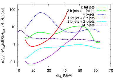
(a)

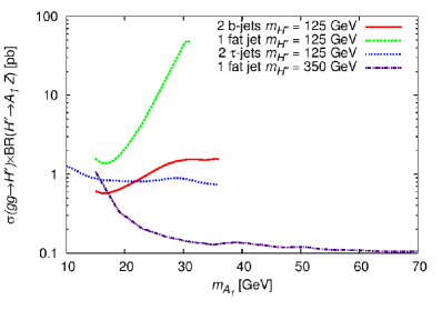
(b)

Figure 1: Expected experimental sensitivities as functions of $m_{A_{1}}$, in various possible final state combinations for (a) the $gg\to H_{\rm SM}\rightarrow A_{1}A_{1}$ process and (b) the $gg\to H^{\prime\prime}\rightarrow A_{1}Z$ process.

4 Results and discussion

In this section we present the numerical results of our analysis. As noted in the Introduction, in the NMSSM $H_{1}$ and $H_{2}$ can both have masses around $125$$\,\mathrm{GeV}$ and SM-like properties, and can thus alternatively play the role of the $H_{\rm SM}$. An SM-like $H_{1}$ with mass around 125$\,\mathrm{GeV}$ can be obtained over wide regions of the CNMSSM-NUHM parameter space, defined in section 2. However, the additional requirement of $m_{A_{1}}\lesssim 150$$\,\mathrm{GeV}$ somewhat constrains these regions. An SM-like $H_{2}$, in contrast, requires much more specific parameter combinations. In the following we discuss the LHC phenomenology of a light $A_{1}$ in the two cases, with $H_{\rm SM}=H_{1}$ and with $H_{\rm SM}=H_{2}$, separately. In principle, in the NMSSM the signal peak observed at the LHC near 125$\,\mathrm{GeV}$ can also be interpreted as a superposition of both $H_{1}$ and $H_{2}$ that are nearly degenerate in massGunion:2012gc ; Gunion:2012he . In such a case the signal rates due to these two Higgs bosons should be combined for testing against the LHC Higgs boson data, depending on the assumed experimental mass resolution. However, in our scans such points occurred very rarely, covering a very insignificant portion of the parameter space. We, therefore, ignore such a possibility in our analysis, assuming the signal rates to be due only to one Higgs boson, the $H_{\rm SM}$ in a given case.

4.1 SM-like $H_{1}$

In figure 2(a) we show the distribution of the mass of $H_{1}$ against that of $A_{1}$ for the points obtained in our scans assuming $H_{\rm SM}=H_{1}$. The ranges of the parameters scanned, are given in table 2. Note that in this and in the following figures we will allow the SM-like Higgs mass to be in the range $122\,\mathrm{GeV}\leq m_{H_{\rm SM}}\leq 129\,\mathrm{GeV}$. This is to take into account the experimental as well possibly large theoretical uncertainties in the model prediction of $m_{H_{\rm SM}}$, given the Higgs boson mass measurement of 125$\,\mathrm{GeV}$ at the LHC. The heat map in the figure corresponds to the parameter $\tan\beta$. One can see a particularly dense population of points for $\tan\beta\sim 1-6$ in the figure, with the mass of $H_{1}$ reaching comparatively larger values than elsewhere. However, $m_{A_{1}}$ for such points almost never falls below $\sim 60$$\,\mathrm{GeV}$. In figure 2(b) we show $m_{H_{1}}$ as a function of the coupling ${\kappa}$, with the heat map corresponding to the coupling ${\lambda}$. Again there is a clear strip of points with ${\lambda}\gtrsim 0.6$ (and ${\kappa}\sim 0.15-0.5$) for which $m_{H_{1}}$ can be as high as 129$\,\mathrm{GeV}$. These points are the ones lying also in the small $\tan\beta$ strip in figure 2(a). The rest of the points, corresponding to smaller ${\lambda}$ and larger $\tan\beta$, can barely yield $m_{H_{1}}$ in excess of 126$\,\mathrm{GeV}$. The reason for the behaviour of $m_{H_{1}}$ observed in these figures is explained in the following.

The tree-level mass of $H_{\rm SM}$ in the NMSSM is given byEllwanger:2009dp

$$m_{H_{\rm SM}}^{2}\simeq m_{Z}^{2}\cos^{2}2\beta+{\lambda}^{2}v^{2}\sin^{2}2\beta-\frac{{\lambda}^{2}v^{2}}{{\kappa}^{2}}\left[{\lambda}-\sin 2\beta\left({\kappa}+\frac{{A_{\lambda}}}{2s}\right)\right]^{2}\,.$$ (10)

For small ${\lambda}$ and large $\tan\beta$ the negative third term on the right hand side of the above equation can dominate over the positive second term, leading to a reduction in the tree-level $m_{H_{\rm SM}}^{2}$. The mass of $H_{\rm SM}$ can then reach values as high as 125$\,\mathrm{GeV}$ or so only through large radiative corrections from the stop sector, thus requiring the so-called maximal mixing scenario and thereby invoking fine-tuning concerns. Alternatively the correct mass of $H_{\rm SM}$, particularly when it is the $H_{1}$, can be obtained in a more natural way through large ${\lambda}$ and small $\tan\beta$, implying a reduced dependence on the radiative corrections. This enhances the tree-level contribution to $m_{H_{\rm SM}}^{2}$ from the positive second term and nullifies that from the negative third term. We shall refer to this parameter configuration as the ‘naturalness limit’ in the following. In figure 3(a) we see that, for the points in the strip corresponding to the naturalness limit, larger $m_{H_{1}}$ is obtained without requiring either ${m_{0}}$  shown on the horizontal axis, or $A_{0}$, shown by the heat map, to be too large. For points outside this strip, the desired mass of $H_{1}$ can only be achieved with large ${m_{0}}$ or, in particular, very large $-|A_{0}|$.

Parameter	Extended range	Reduced range
${m_{0}}$ (GeV)	200 – 4000	200 – 2000
$m_{1/2}$ (GeV)	100 – 2000	100 – 1000
$A_{0}$ (GeV)	$-5000$ – 0	$-3000$ – 0
$\mu_{\rm{eff}}$ (GeV)	100 – 2000	100 – 200
$\tan\beta$	1 – 40	1 – 6
${\lambda}$	0.01 – 0.7	0.4 – 0.7
${\kappa}$	0.01 – 0.7	0.01 – 0.7
${A_{\lambda}}$∗ (GeV)	$-2000$ – 2000	$-500$ – 500
${A_{\kappa}}$∗ (GeV)	$-2000$ – 2000	$-500$ – 500

Table 2: Ranges of the CNMSSM-NUHM input parameters scanned for obtaining a $\sim 125$$\,\mathrm{GeV}$ $H_{\rm SM}$ along with a light $A_{1}$.

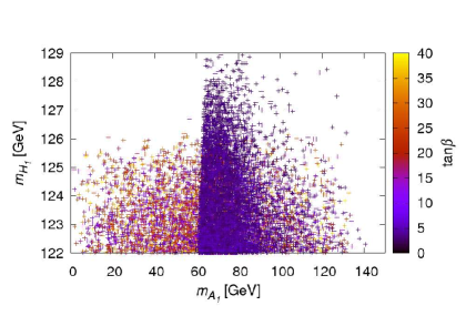
(a)

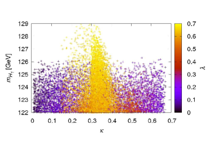
(b)

Figure 2: Case with $H_{\rm SM}=H_{1}$: (a) Mass of $H_{1}$ vs. that of $A_{1}$, with the heat map showing the distribution of $\tan\beta$; (b) $m_{H_{1}}$ as a function of the parameter ${\kappa}$, with the heat map showing the distribution of the coupling ${\lambda}$.

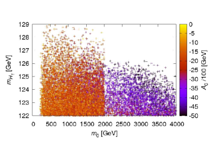
(a)

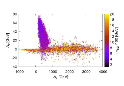
(b)

Figure 3: Case with $H_{\rm SM}=H_{1}$: (a) Mass of $H_{1}$ as a function of the parameter ${m_{0}}$, with the heat map showing the distribution of the soft trilinear coupling $A_{0}$; (b) the parameter ${A_{\lambda}}$ vs. the parameter ${A_{\kappa}}$  with the heat map showing the distribution of the soft mass $m_{1/2}$.

In figure 3(b) we show the distributions of the remaining three parameters, ${A_{\lambda}}$, ${A_{\kappa}}$ and $m_{1/2}$, on the horizontal and vertical axes and by the heat map, respectively. Again one sees a dense strip of points with relatively smaller values of $m_{1/2}$  which corresponds to the naturalness limit. These points are also restricted to comparatively smaller values of $+|{A_{\lambda}}|$ but extend to a wider range of ${A_{\kappa}}$ than the points outside the strip. The smallness and positivity of ${A_{\lambda}}$ is warranted for further enhancing the tree-level $m_{H_{\rm SM}}^{2}$ by reducing the size of the term in the square brackets in eq. (10). The sign and size of ${A_{\kappa}}$ is then mainly defined by the condition of smallness of $m_{A_{1}}$. According to eq. (4), for ${A_{\lambda}},{A_{\kappa}}>0$, increasing ${A_{\kappa}}$ reduces $m^{2}_{A_{1}}$ as long as $|2{\lambda}\ v^{2}\sin 2\beta|<|3s{A_{\kappa}}|$. Moreover, since ${\lambda}$ and $\tan\beta$ ought to be large in order to maximise $m_{H_{1}}$, $m_{A_{1}}$ can only be reduced further by reducing ${\kappa}$.

However, going back to the figure 2(a), it is evident that $A_{1}$ never has a mass below $m_{H_{1}}/2$ in the naturalness limit, as $m_{A_{1}}$ cuts off sharply at that value. The reason for this is that the tree-level $H_{i}A_{1}A_{1}$ couplings are proportional to $\lambda^{2}$ (see eq. (A.17) inEllwanger:2009dp ). Thus, for very large ${\lambda}$, required to enhance the mass of $H_{1}$, when $m_{A_{1}}<m_{H_{1}}/2$, the $H_{1}\to A_{1}A_{1}$ decay can be highly dominant over the other $H_{1}$ decay channels. In fact the BR($H_{1}\to A_{1}A_{1}$) reaches unity for such points, resulting in highly suppressed BRs for all other channels. Consequently the signal rates of $H_{1}$ in the $\gamma\gamma$ and $ZZ$ channels drop to unacceptably low values and the corresponding points are rejected during our scans. This can in fact be used to constrain the decay of $H_{\rm SM}$ to lighter scalars or pseudoscalarsCao:2013gba .

4.1.1 $bbA_{1}$ production

We first analyse the $bbA_{1}$ production process for this case. In figure 4 we show the total cross section, $\sigma(gg\rightarrow bbA_{1})$, as a function of $m_{A_{1}}$ for all the good points from our scan. The red and blue points in the figure are the ones for which the calculated $R_{X}$ lies within the range of $\mu_{X}$ measured by CMS and ATLAS, respectively. The green points are then the ‘unfiltered’ ones for which neither of these two constraints are satisfied. We shall retain this color convention for all the figures showing cross sections henceforth. One notices in the figure that none of the points with $m_{A_{1}}$ below $\sim 60$$\,\mathrm{GeV}$ satisfies the ATLAS constraints on $R_{X}$, while some of these comply with the CMS ones. This is due to the fact that all these points belong outside the naturalness limit, and hence possess very (MS)SM like characteristics. According to eq. (8), the ATLAS measurements of $\mu_{\gamma\gamma}$ and $\mu_{ZZ}$ are substantially higher than 1. Such high rates in the $\gamma\gamma$ and $ZZ$ channels can only be obtained in the naturalness limit of the NMSSM, as noted inEllwanger:2011aa . Hence one sees a large number of points corresponding to the naturalness limit consistent with the ATLAS constraint in the figure. Note also that the ATLAS collaboration has recently updated its measurement of $\mu_{\gamma\gamma}$Aad:2014eha , which is now comparatively closer to the SM prediction. However, no updates on $\mu_{ZZ}$ for the same data set have been released. This implies that even if we use the newly released $\mu_{\gamma\gamma}$ value, $R_{ZZ}$ for a given point still ought to be large to satisfy the older $\mu_{ZZ}$ range from ATLAS.

Also shown in figure 4 are the sensitivity curves corresponding to the $2b2\tau$ and $4b$ final states for an expected integrated luminosity of 3000/fb at the LHC. We see that none of the good points from the scan have a cross section large enough to be discoverable in any of the considered final state combinations. This may seem to be in contrast with the results of earlier studiesAlmarashi:2010jm ; Almarashi:2011hj . However, a closer inspection of these previous results reveals that for all the model points yielding a potentially detectable $A_{1}$, $m_{H_{1}}$ is always below 120$\,\mathrm{GeV}$. To further verify this observation, we performed a test scan of the NMSSM parameter space with an earlier version (2.3.1) of the NMSSMTools package and checked the surviving points with version 4.2.1 as well as with HiggsBounds. We noted that all the points with a large $bbA_{1}$ cross section obtained in the test scan were indeed ruled out by the latest data from the Higgs searches at LEP and LHC. In addition to that, the improvements in the calculation of the Higgs boson masses and reduced couplings in the newer version may also be responsible for a more accurate theoretical prediction of the cross section for this process.

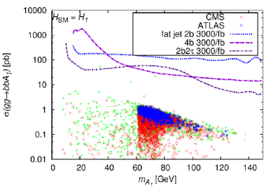
Figure 4: $b\bar{b}A_{1}$ production cross section as a function of $m_{A_{1}}$ in the case with $H_{\rm SM}=H_{1}$. The red and the blue points satisfy the CMS and the ATLAS constraints on $R_{\gamma\gamma/ZZ}$, respectively. In green are the unflitered points satisfying neither of these constraints. Also shown are the sensitivity curves for various final state combinations. See text for details.

4.1.2 Production via $H_{\rm SM}\rightarrow A_{1}A_{1}/Z$

Among the indirect production channels, we first analyse the $H_{1}\rightarrow A_{1}A_{1}$ and $H_{1}\rightarrow A_{1}Z$ processes. As noted above in detail, for the points in the naturalness limit, $m_{A_{1}}$ never falls below $m_{H_{1}}/2$, making both these processes kinematically irrelevant. This decay is then only possible for points obtained outside this limit, i.e., for small ${\lambda}$ and large $\tan\beta$.

In figure 5(a), we show the total cross section for the $gg\rightarrow H_{1}\rightarrow A_{1}A_{1}$ channel. Also shown in the figure are the curves corresponding to the sensitivity reaches in the $2b2\tau$ as well as the $4\tau$ final states. For the $2b2\tau$ curve, we have used a combination of the fat jet plus two $\tau$-jets and the two single $b$-jets plus two $\tau$-jets analyses. The fat jet analysis has been used for low masses while the two single $b$-jets analysis has been used when it becomes more sensitive. The curve corresponding to the $4\tau$ final state extends to lower $m_{A_{1}}$. This is because, for $m_{A_{1}}<10$ GeV, the $A_{1}\to b\bar{b}$ decay becomes kinematically disallowed, resulting in the $4\tau$ being the only applicable channel and causing BR$(A_{1}\to\tau^{+}\tau^{-})$ to rise from near 0.1 to around 0.9, thereby causing a sharp dip in the $4\tau$ sensitivity curve. We note in the figure that while a lot of unfiltered points should be accessible at the LHC in the $2b2\tau$ final state at $\mathcal{L}=300$/fb, very few points consistent with the CMS constraint on $R_{X}$ lie above the corresponding curve. None of the points consistent with the corresponding ATLAS constraints appears in this figure, for reasons noted earlier.

In figure 5(b) we see that the $A_{1}Z$ channel will not be accessible at the LHC in any final state combination even for the maximum integrated luminosity assumed. All the points where $m_{A_{1}}$ is low enough for this decay channel to be relevant lie much below the sensitivity curves shown, which correspond to the two single $b$-jets plus $\ell^{+}\ell^{-}$ and the two $\tau$-jets plus $\ell^{+}\ell^{-}$ final states. This is due to the fact that the BR$(H_{1}\to A_{1}Z)$ is extremely small for such points. The reason for the smallness of this BR can be understood by examining the $H_{i}A_{j}Z$ couplings, which are proportional to the factors $S_{i1}P_{j1}-S_{i2}P_{j2}$ (see eq. (A.17) inEllwanger:2009dp ). Here $S_{i1}$ and $S_{i2}$ are the terms corresponding to the $H_{dR}$ and $H_{uR}$ weak eigenstates in the scalar mixing matrix, and $P_{j1}$ and $P_{j2}$ are the terms corresponding to $H_{dI}$ and $H_{uI}$ weak eigenstates in the pseudoscalar mixing matrix, with the indices $R$ and $I$ referring to the real and imaginary parts, respectively, of the complex Higgs fields. Owing to the structure of the scalar and the pseudoscalar mass matrices, $P_{j1}/P_{j2}=\tan\beta$ for the singlet-like $A_{j}$, and for a very SM-like $H_{i}=H_{\rm SM}$, $S_{i2}/S_{i1}\approx\tan\beta$. This causes the factor $S_{i1}P_{j1}-S_{i2}P_{j2}$ to approach zero, resulting in an almost vanishing $H_{1}A_{1}Z$ coupling.

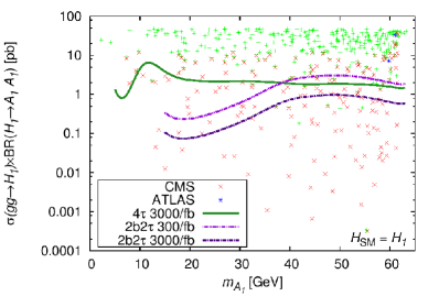
(a)

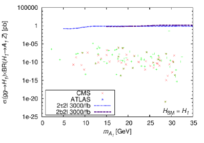
(b)

Figure 5: Total cross sections in the case with $H_{\rm SM}=H_{1}$ for (a) the $gg\to H_{\rm SM}\to A_{1}A_{1}$ process and (b) the $gg\to H_{\rm SM}\to A_{1}Z$ process. The color convention for the points is the same as in figure 4. See text for details about the sensitivity curves.

4.1.3 Production via $H^{\prime}\rightarrow A_{1}A_{1}/Z$

We next consider the decays of the other non-SM-like Higgs bosons in the $A_{1}A_{1}$ and $A_{1}Z$ channels. In figure 6(a) and (b) we see that the situation for the $H_{2}\to A_{1}A_{1}/Z$ decays is very similar to that for the $H_{1}\to A_{1}A_{1}/Z$ decays, respectively. The sensitivity curves shown correspond to the same final state combinations as those in figure 5(a) and (b). But here the difference is that the combined invariant mass of the final state particles is not required to be $\sim 125$$\,\mathrm{GeV}$. The $H_{2}$ mass used in the lines for the $H_{2}\to A_{1}A_{1}$ decay is 175$\,\mathrm{GeV}$, while for the $H_{2}\to A_{1}Z$ channel we use 200$\,\mathrm{GeV}$ in order to cover the whole populated region of panel (b). The actual $H_{2}$ mass for the points shown ranges from around 130$\,\mathrm{GeV}$ to around 300$\,\mathrm{GeV}$, with a large population below 150$\,\mathrm{GeV}$, so for some points the sensitivities shown might be somewhat overestimated.

We note that, although the prospects for the $H_{2}\to A_{1}A_{1}$ channel are not great, they are slightly better than those for the $H_{1}\to A_{1}A_{1}$ mode seen above. For the former, a significant number of points satisfying also the ATLAS constraints on $R_{X}$ may be probed in the $b\bar{b}\tau^{+}\tau^{-}$ final state combination, contrary to what was observed for the latter. The $H_{2}\to A_{1}Z$ channel, on the other hand, will not be accessible at all in any final state combination even at 3000/fb integrated luminosity. This is not surprising given the singlet-like natures of both $A_{1}$ and $H_{2}$.

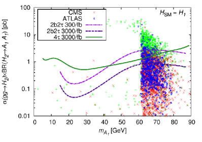
(a)

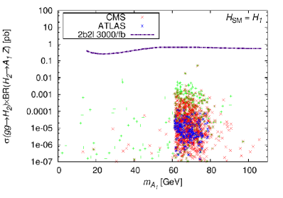
(b)

Figure 6: Total cross sections in the case with $H_{\rm SM}=H_{1}$ for (a) the $gg\to H_{2}\to A_{1}A_{1}$ process and (b) the $gg\to H_{2}\to A_{1}Z$ process. The color convention for the points is the same as in figure 4. See text for details about the sensitivity curves.

In the case of $H_{3}$ decays the overall prospects are quite different from those noted for the lighter scalars above. In figure 7(a) one can see that the $H_{3}\to A_{1}A_{1}$ channel will be inaccessible even for maximum assumed luminosity. The sensitivity curves shown correspond to an $H_{3}$ mass of 350$\,\mathrm{GeV}$ and a combination of the fat jet and the two single $b$-jets analyses, which always shows the highest possible reach for a given $m_{A_{1}}$. The reason for the poor prospects in the $H_{3}\to A_{1}A_{1}$ channel is to a large extent a consequence of the high mass of $H_{3}$, partly because such a mass reduces the production cross section and partly because a number of other decay channels like $t\bar{t}$, $W^{+}W^{-}$, $ZZ$ and lighter Higgs scalars are available. These other channels are relatively unsuppressed and hence dominate over the $A_{1}A_{1}$ channel.

In figure 7(b) we see that, in contrast, the $H_{3}\to A_{1}Z$ channel shows some promise. A fraction of the points lies above the $\mathcal{L}=3000$/fb sensitivity curve corresponding to the $2b2\ell$ final state, with one point lying above the 300/fb curve. Most of these points satisfy the CMS and/or ATLAS constraints on $R_{X}$. The total cross section for this process can reach detectable levels due to the fact that the $H_{3}A_{1}Z$ coupling is not subject to the peculiar cancellation noted earlier for the $H_{1}A_{1}Z$ coupling. Since $A_{1}$ with mass larger than $\sim 60$$\,\mathrm{GeV}$ will not be accessible in any other production mode, this channel will be very crucial for its discovery, which may be possible even at 300/fb integrated luminosity at the LHC.

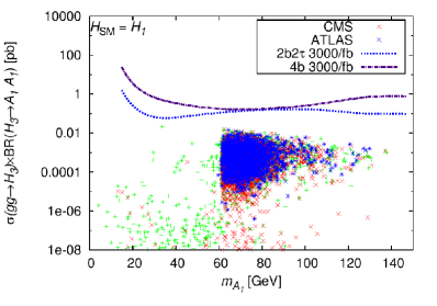
(a)

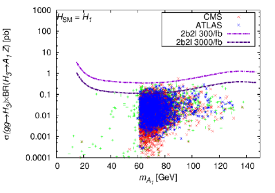
(b)

Figure 7: Total cross sections in the case with $H_{\rm SM}=H_{1}$ for (a) the $gg\to H_{3}\to A_{1}A_{1}$ process and (b) the $gg\to H_{3}\to A_{1}Z$ process. The color convention for the points is the same as in figure 4. See text for details about the sensitivity curves.

4.2 SM-like $H_{2}$

For the case $H_{\rm SM}=H_{2}$, we noted in the initial wide-ranged scans that a vast majority of the points with $m_{H_{2}}\sim 125$$\,\mathrm{GeV}$ that survived the constraints imposed within NMSSMTools  corresponded to the naturalness limit. We therefore performed a dedicated scan of the reduced parameter ranges seen in table 2, and will only analyse such points here. Contrary to the $H_{\rm SM}=H_{1}$ case, here $m_{A_{1}}$ can be much smaller even in the naturalness limit, as seen in figure 8(a), where we show the distribution of $m_{A_{1}}$ against that of $m_{H_{2}}$, with the heat map corresponding to the parameter $\tan\beta$. One sees in the figure that lower values of $m_{A_{1}}$ prefer slightly larger values of $\tan\beta$. In figure 8(b) we note that $m_{A_{1}}$ falls also with decreasing ${\lambda}$, shown by the heat map.

An important thing to note here is that, despite the comparatively smaller ${\lambda}$ and larger $\tan\beta$, $m_{H_{2}}$ in this case can easily reach as high as 129$\,\mathrm{GeV}$. This is because, as explained inBadziak:2013bda , the mixing of the SM-like $H_{2}$ with the lighter singlet-like $H_{1}$ can result in a 6–8$\,\mathrm{GeV}$ raise in the tree-level mass of $H_{2}$, even for moderate values of $\tan\beta$ and ${\lambda}$. Such relatively small ${\lambda}$ and small-to-moderate $\tan\beta$, together with small ${\kappa}$, as observed in the heat map of figure 9(a), in turn also help reduce $m_{A_{1}}$. Importantly also, $m_{A_{1}}$ in this case can reach comparatively much smaller values without such points being severely constrained due to the opening of the $H_{\rm SM}\to A_{1}A_{1}$ channel, as was noted for the $H_{\rm SM}=H_{1}$ case. The relatively smaller values of ${\lambda}$ imply that the BR($H_{\rm SM}\to A_{1}A_{1}$) never gets overwhelming enough to completely diminish the other BRs and consequently the signal rates of $H_{2}$ in the $\gamma\gamma$ and $ZZ$ channels. However, the onset of the $H_{2}\to A_{1}A_{1}$ channel does suppress points with large ${\lambda}$ below $M_{H_{2}}/2$ and hence gives rise to sharp separations between the violet and orange regions in figure 8(a) and (b).

In figure 9(b) one sees that ${A_{\lambda}}$ is always positive although the mass of $A_{1}$, shown by the heat map, is almost independent of ${A_{\lambda}}$, while ${A_{\kappa}}$ can be both negative and positive. Furthermore, $m_{A_{1}}$ clearly falls with increasing $+|{A_{\kappa}}|$ (and, equivalently, decreasing $-|{A_{\kappa}}|$), which is again in accordance with eq. (4).

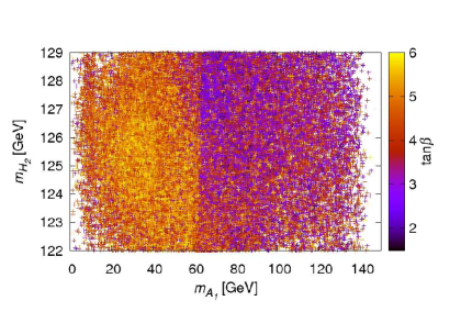
(a)

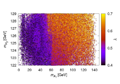
(b)

Figure 8: Mass of $H_{2}$ vs. that of $A_{1}$ for the case with $H_{\rm SM}=H_{2}$. The heat map shows (a) the distribution of $\tan\beta$ and (b) the distribution of ${\lambda}$.

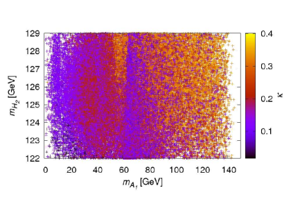
(a)

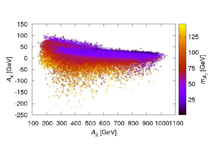
(b)

Figure 9: Case with $H_{\rm SM}=H_{2}$: (a) mass of $H_{2}$ vs. that of $A_{1}$, with the heat map showing the distribution of ${\kappa}$; (b) the parameter ${A_{\lambda}}$ vs. the parameter ${A_{\kappa}}$  with the heat map showing the distribution of the mass of $A_{1}$.

4.2.1 $bbA_{1}$ production

In figure 10 we show the $gg\rightarrow bbA_{1}$ rates for all the good points from the scan for this case. The sensitivity curves shown correspond to the $2b2\tau$ and $4b$ final states for an expected integrated luminosity of 3000/fb at the LHC. As in the case with $H_{\rm SM}=H_{1}$ discussed above, none of the good points from the scan have a cross section large enough to be discoverable in any of the final state combinations.

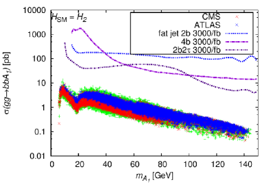
Figure 10: $b\bar{b}A_{1}$ production cross section as a function of $m_{A_{1}}$ in the case with $H_{\rm SM}=H_{2}$. The color convention for the points is the same as in figure 4. See text for details about the sensitivity curves.

4.2.2 Production via $H_{\rm SM}\rightarrow A_{1}A_{1}/Z$

In figure 11(a) we show the prospects for the $H_{2}\to A_{1}A_{1}$ channel when $H_{2}$ is SM-like. The sensitivity lines shown correspond to the same final state combinations as in figure 5, with the addition of a line for the $2b2\tau$ final state at $\mathcal{L}=30$/fb. We see that, compared with the $H_{\rm SM}=H_{1}$ case, a much larger part of the parameter space can be probed in this channel at the LHC, even at as low as 30/fb integrated luminosity. The reason is clearly that in this case the points with $m_{A_{1}}<m_{H_{\rm SM}}/2$ belong to the lower edge of the naturalness limit (${\lambda}\sim 0.4$), where BR($H_{2}\to A_{1}A_{1}$) is sufficiently enhanced without causing the $H_{\rm SM}$ for these points to deviate too much from a SM-like behaviour. This is the reason why a large fraction of the points with large cross section is consistent also with the CMS and ATLAS measurements of $\mu_{\gamma\gamma/ZZ}$.

In figure 11(b) we see that the prospects in the $H_{2}\to A_{1}Z$ channel are still poor. They are, nevertheless, much better than when $H_{SM}=H_{1}$, despite the same peculiar cancellation in the $H_{i}A_{j}Z$ couplings discussed earlier. Here this cancellation is not as exact because the relation $S_{i2}/S_{i1}\approx\tan\beta$ is not satisfied as strictly.

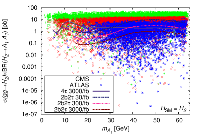
(a)

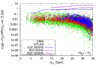
(b)

Figure 11: Total cross sections in the case with $H_{\rm SM}=H_{2}$ for (a) the $gg\to H_{\rm SM}\to A_{1}A_{1}$ process and (b) the $gg\to H_{\rm SM}\to A_{1}Z$ process. The color convention for the points is the same as in figure 4. See text for details about the sensitivity curves.

4.2.3 Production via $H^{\prime}\rightarrow A_{1}A_{1}/Z$

The prospects for the discovery of a light pseudoscalar in the $H_{1}\to A_{1}A_{1}$ and $H_{1}\to A_{1}Z$ decay channels, for a singlet-like $H_{1}$, are illustrated in figures 12(a) and (b), respectively. In the panel (a) the sensitivity curves correspond to the one fat jet plus two $\tau$-jets, the two single $b$-jets plus two $\tau$-jets and the $4\tau$ final states. These are compared with the cross sections of the good points from the scans. For the fat jet plus two $\tau$-jets as well as the $4\tau$ curves $m_{H_{1}}=100$$\,\mathrm{GeV}$, while for the two $b$-jets plus two $\tau$-jets curve $m_{H_{1}}=125$$\,\mathrm{GeV}$, which allows the coverage of points with large $m_{A_{1}}$. However, in neither of these cases is the mass used to constrain the kinematics. The $4\tau$ line has been added since, for $m_{A_{1}}<2m_{b}$, the $A_{1}$ can only be accessed via this channel. Understandably, this line is cut off at the kinematical upper limit of $m_{H_{1}}/2=50$$\,\mathrm{GeV}$. The lines corresponding to the fat jet analysis are cut off where the efficiency for extracting the signal becomes too bad for the result to be reliable.

One sees in figure 12(a) that almost all the points complying with the current CMS and/or ATLAS constraints on $R_{X}$ are potentially discoverable, even at $\mathcal{L}=30$/fb. Thus a large part of the scanned NMSSM parameter space can be probed via this decay channel. In particular, since such light pseudoscalars cannot be obtained in the naturalness limit for the case with $H_{\rm SM}=H_{1}$, it should essentially be possible to exclude $m_{A_{1}}\lesssim 60$$\,\mathrm{GeV}$ in the natural NMSSM at the LHC via this channel. Although a light $A_{1}$ may still be obtained with slightly smaller ${\lambda}$  it will be difficult for $H_{\rm SM}$ to reach $\sim 125$$\,\mathrm{GeV}$ without large radiative corrections. Note also that such an exclusion will not cover the narrow regions of the parameter space where the $A_{1}\to H_{1}H_{1}$ decay is kinematically allowed. Finally, In figure 12(b), we see that the prospects for the discovery of $A_{1}$ via the $H_{1}\to A_{1}Z$ channel are non-existent in this case too.

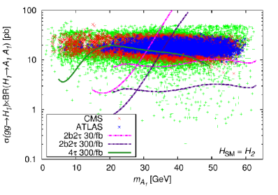
(a)

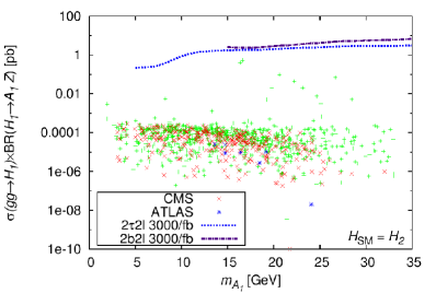
(b)

Figure 12: Total cross sections in the case with $H_{\rm SM}=H_{2}$ for (a) the $gg\to H_{1}\to A_{1}A_{1}$ process and (b) the $gg\to H_{1}\to A_{1}Z$ process. The color convention for the points is the same as in figure 4. See text for details about the sensitivity curves.

For the decay chain starting from $H_{3}$, the situation is similar to the one in the case with $H_{\rm SM}=H_{1}$. In figure 13(a) we see that the $H_{3}\to A_{1}A_{1}$ channel is inaccessible here also due to the fact that, as mentioned before, for such high masses the production cross section gets diminished. Moreover, other decay channels of $H_{3}$ dominate over this channel. The sensitivity curves in the figure correspond to the $2b2\tau$ and $4\tau$ final states for $\mathcal{L}=3000$/fb. In fact, the cross sections obtainable here are even marginally smaller than those seen earlier for the $H_{3}\to A_{1}A_{1}$ channel in the $H_{\rm SM}=H_{1}$ case, owing, again, to the generally smaller values of ${\lambda}$ in this case.

Conversely, the $H_{3}\to A_{1}Z$ channel, shown in figure 13, shows much more promise than before. As pointed out before, this has to do with the increased sensitivity in the fat jet analysis when the involved masses are high, as well as the relatively large $H_{3}A_{1}Z$ coupling, which is actually somewhat larger here than in the $H_{\rm SM}=H_{1}$ case, due to a somewhat larger doublet component of $A_{1}$. Again, there are hardly any points with $m_{A_{1}}<m_{H_{\rm SM}}/2$ for ${\lambda}$ large enough to yield a high total cross section, for the same reasons as discussed earlier. We emphasise again that this channel will be an extremely important probe for an NMSSM $A_{1}$ with mass greater than $\sim 60$$\,\mathrm{GeV}$.

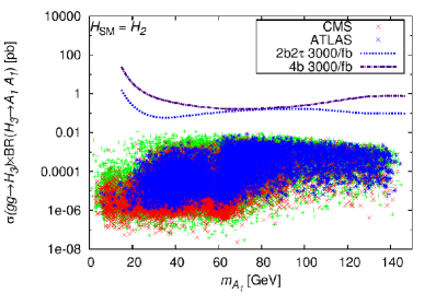
(a)

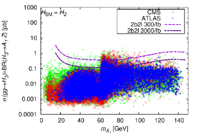
(b)

Figure 13: Total cross sections in the case with $H_{\rm SM}=H_{1}$ for (a) the $gg\to H_{3}\to A_{1}A_{1}$ process and (b) the $gg\to H_{3}\to A_{1}Z$ process. The color convention for the points is the same as in figure 4. See text for details about the sensitivity curves.

4.3 Benchmark points

As pointed out in the previous sections, of the channels discussed in this paper, $gg\to H_{3}\to A_{1}Z$ appears to be the only one in which an $A_{1}$ lying in the interval $\sim 60\,\mathrm{GeV}$–$120$$\,\mathrm{GeV}$ could be discovered with 300/fb integrated luminosity at the LHC. Note though that the $H^{\pm}\to A_{1}W^{\pm}$ channel has also been found to be of interest for such pseudoscalar massesDas:2014fha .

While the $H_{i}\to A_{1}A_{1}$ decay channel has been previously visited in the literature, this channel has not been emphasised upon much. Therefore, in order to facilitate further investigation of this channel, we single out a few benchmark points that should be within the reach of the LHC at $\mathcal{L}=300$/fb, and provide their details in table 3. Besides yielding large cross sections for this channel, these points also satisfy the CMS and/or ATLAS constraints on $R_{X}$. Point 1 corresponds to the case with $H_{\rm SM}=H_{1}$, while Points 2, 3 and 4 correspond to the $H_{\rm SM}=H_{2}$ case and are intended to cover the entire accessible range of $m_{A_{1}}$.

Case	$H_{\rm SM}=H_{1}$	$H_{\rm SM}=H_{2}$
	Point 1	Point 2	Point 3	Point 4
Input parameters
${m_{0}}$ (GeV)	991.42	1321.2	1817.8	1358.1
$m_{1/2}$ (GeV)	737.59	752.07	977.07	947.62
$A_{0}$ (GeV)	$-729.51$	$-88.81$	$-1112.88$	$-699.12$
$\mu_{\rm{eff}}$ (GeV)	172.43	150.52	167.17	185.77
$\tan\beta$	1.807	1.636	1.661	1.549
${\lambda}$	0.66	0.619	0.6248	0.5978
${\kappa}$	0.1772	0.0692	0.0506	0.1096
${A_{\lambda}}$∗ (TeV)	59.136	426.49	$-466.9$	$-115.9$
${A_{\kappa}}$∗ (TeV)	474.85	444.7	$-142.41$	275.31
Observables
$m_{A_{1}}$ (GeV)	89.88	106.22	73.71	63.95
$m_{H_{1}}$ (GeV)	127.1	85.1	94.7	116.4
$m_{H_{2}}$ (GeV)	130.3	124.8	126.85	125.41
$m_{H_{3}}$ (GeV)	378.47	327.85	360.58	388.21
$R_{\gamma\gamma}$	1.156	1.114	0.964	1.099
$R_{ZZ}$	0.824	1.063	0.982	0.972
$\sigma\times{\rm BR}(H_{3}\to A_{1}Z)$ (pb)	0.57	1.33	1.47	0.83

Table 3: Some specifics of the four benchmark points for the $gg\to H_{3}\to A_{1}Z$ channel.

5 Conclusions

In this article we have revisited the discovery prospects of a light NMSSM pseudoscalar, $A_{1}$, at the forthcoming 14$\,\mathrm{TeV}$ LHC run. We have shown the dependence of the mass expression for $A_{1}$ on the input parameters of the model and discussed its most prominent production and decay modes. Through scans of the CNMSSM-NUHM parameter space, we have identified the regions where $A_{1}$ with mass $\lesssim 150$$\,\mathrm{GeV}$ can be obtained while requiring one of the two light CP-even Higgs bosons to have a mass around 125$\,\mathrm{GeV}$ and SM-like signal rates. We have then discussed in detail the salient features of these regions, separately for the case when the SM-like Higgs boson is $H_{1}$ and the case when it is $H_{2}$.

To connect to LHC physics we have performed detailed MC analyses of the various $A_{1}$ production channels of interest. These channels can be divided into direct and indirect ones, with the former referring to the $b\bar{b}$-associated production mode and the latter encompassing the decays of the heavier CP-even Higgs bosons into $A_{1}A_{1}$ or $A_{1}Z$ pairs. The $A_{1}$ thus produced is assumed to decay via the channels with the highest BRs, i.e., $b\bar{b}$ and $\tau^{+}\tau^{-}$, while the $Z$ boson decays leptonically. For the $A_{1}\to b\bar{b}$ decays, we have adopted a jet substructure method, which improves the experimental sensitivity for a low mass $A_{1}$ through boosted $b$-jet pairs and is particularly useful for the decays of the heavy CP-even Higgs bosons.

We have found that, contrary to the findings of some earlier studies, the direct production channel, $bbA_{1}$, has now been rendered ineffective by the observed properties of the SM-like Higgs boson discovered at the LHC. However, some of the indirect production channels still show plenty of promise. Specifically, the decays of the scalars, including in particular the SM-like Higgs boson, whether $H_{1}$ or $H_{2}$, carry the potential to reveal an $A_{1}$ with mass $\lesssim 60$$\,\mathrm{GeV}$ for the integrated luminosity at the LHC as low as 30/fb. In case of non-discovery, this channel could help practically exclude large portions of the NMSSM parameter space. This is particularly true when the SM-like $H_{2}$ is required to achieve a mass close to 125$\,\mathrm{GeV}$ in a natural way (without needing large radiative corrections), while the $H_{1}$ is not light enough to allow $A_{1}$ decays into its pairs.

Most notably though, when the $A_{1}$ is heavier than $\sim 60$$\,\mathrm{GeV}$, while its pair production via decays of the two lightest CP-even Higgs bosons also becomes inaccessible, the $gg\to H_{3}\to A_{1}Z$ channel takes over as the most promising one. This channel is, therefore, of great importance and warrants dedicated probes in future analyses at the LHC. We strongly advocate such studies, for which we have provided details of some benchmark points which give significantly large $gg\to H_{3}\to A_{1}Z$ cross sections and at the same time show consistency with the current data from the LHC Higgs boson searches.

We summarise all our findings in table 4, quoting the integrated luminosity at which a reasonable number of model points should be discoverable at the LHC in at least one of the given final state combinations. Also given are the mass ranges of $A_{1}$ over which the discovery in a given production channel is plausible.

Production mode	Final states	Accessibility, for $\mathcal{L}$	Mass range (GeV)
$b\bar{b}A_{1}$	$4b$, $2b2\tau$	x
$H_{1}\to A_{1}A_{1}$ ($H_{1}=H_{\rm SM}$)	$4b$, $2b2\tau$, $4\tau$	✓ 300/fb	$m_{A_{1}}<63$
$H_{1}\to A_{1}A_{1}$ ($H_{2}=H_{\rm SM}$)	$4b$, $2b2\tau$, $4\tau$	✓ 30/fb	$m_{A_{1}}<60$
$H_{1}\to A_{1}Z$	$2b2\ell$, $2\tau 2\ell$	x
$H_{2}\to A_{1}A_{1}$ ($H_{1}=H_{\rm SM}$)	$4b$, $2b2\tau$, $4\tau$	✓ 300/fb	$60<m_{A_{1}}<80$
$H_{2}\to A_{1}A_{1}$ ($H_{2}=H_{\rm SM}$)	$4b$, $2b2\tau$, $4\tau$	✓ 30/fb	$m_{A_{1}}<63$
$H_{2}\to A_{1}Z$	$2b2\ell$, $2\tau 2\ell$	x
$H_{3}\to A_{1}A_{1}$	$4b$, $2b2\tau$, $4\tau$	x
$H_{3}\to A_{1}Z$	$2b2\ell$, $2\tau 2\ell$	✓ 300/fb	$60<m_{A_{1}}<120$

Table 4: List of the $A_{1}$ production channels included in this study. The second column shows the final state combinations of interest for each channel, while the third column shows the integrated luminosity at which the $A_{1}$ can be accessible at the LHC in at least one of these combinations. In the fourth column we provide the mass range within which a signature of $A_{1}$ can be established in the given channel.

Finally, the discovery prospects of the NMSSM Higgs bosons, including also via their decays into other Higgs states, were studied recently inKing:2014xwa . The cross sections calculated by us are generally consistent with those provided there, in the cases where a comparison is meaningful. Furthermore, in that study some points with unusually large BR$(A_{1}\to\gamma\gamma)$ have been emphasised. For some of these points the $2b2\gamma$ final state has been found to be interesting. However, due possibly to the fact that we analyse a different model, the CNMSSM-NUHM, as compared to the phenomenological NMSSM studied inKing:2014xwa , we did not see any points with substantial BR$(A_{1}\to\gamma\gamma)$ in our scans. Hence we did not consider the $2b2\gamma$ final state in our analyses.

ACKNOWLEDGMENTS

This work has been funded in part by the Welcome Programme of the Foundation for Polish Science. S. Moretti is supported in part through the NExT Institute. S. Munir is supported in part by the Swedish Research Council under contracts 2007-4071 and 621-2011-5107. L. Roszkowski is also supported in part by an STFC consortium grant of Lancaster, Manchester and Sheffield Universities. The use of the CIS computer cluster at NCBJ is gratefully acknowledged.

References

- (1) P. Fayet, Supergauge Invariant Extension of the Higgs Mechanism and a Model for the electron and Its Neutrino, Nucl.Phys. B90 (1975) 104–124.
- (2) J. R. Ellis, J. Gunion, H. E. Haber, L. Roszkowski, and F. Zwirner, Higgs Bosons in a Nonminimal Supersymmetric Model, Phys.Rev. D39 (1989) 844.
- (3) L. Durand and J. L. Lopez, Upper Bounds on Higgs and Top Quark Masses in the Flipped SU(5) x U(1) Superstring Model, Phys.Lett. B217 (1989) 463.
- (4) M. Drees, Supersymmetric Models with Extended Higgs Sector, Int.J.Mod.Phys. A4 (1989) 3635.
- (5) D. Miller, R. Nevzorov, and P. Zerwas, The Higgs sector of the next-to-minimal supersymmetric standard model, Nucl.Phys. B681 (2004) 3–30, [hep-ph/0304049].
- (6) ATLAS Collaboration, G. Aad et al., Observation of a new particle in the search for the Standard Model Higgs boson with the ATLAS detector at the LHC, Phys.Lett. B716 (2012) 1–29, [arXiv:1207.7214].
- (7) CMS Collaboration, S. Chatrchyan et al., Observation of a new boson at a mass of 125 GeV with the CMS experiment at the LHC, Phys.Lett. B716 (2012) 30–61, [arXiv:1207.7235].
- (8) CLEO Collaboration, W. Love et al., Search for Very Light CP-Odd Higgs Boson in Radiative Decays of Upsilon(S-1), Phys.Rev.Lett. 101 (2008) 151802, [arXiv:0807.1427].
- (9) E391a Collaboration, Y. Tung et al., Search for a light pseudoscalar particle in the decay , Phys.Rev.Lett. 102 (2009) 051802, [arXiv:0810.4222].
- (10) BaBar collaboration, J. Lees et al., Search for di-muon decays of a low-mass Higgs boson in radiative decays of the , Phys.Rev. D87 (2013), no. 3 031102, [arXiv:1210.0287].
- (11) BaBar Collaboration, J. Lees et al., Search for a low-mass scalar Higgs boson decaying to a tau pair in single-photon decays of , Phys.Rev. D88 (2013), no. 7 071102, [arXiv:1210.5669].
- (12) BaBar Collaboration, J. Lees et al., Search for a light Higgs boson decaying to two gluons or in the radiative decays of , Phys.Rev. D88 (2013), no. 3 031701, [arXiv:1307.5306].
- (13) BABAR Collaboration, I. Peruzzi, Recent BABAR results on dark matter and light Higgs searches and on CP and T violation, EPJ Web Conf. 71 (2014) 00108.
- (14) F. Domingo, U. Ellwanger, E. Fullana, C. Hugonie, and M.-A. Sanchis-Lozano, Radiative Upsilon decays and a light pseudoscalar Higgs in the NMSSM, JHEP 0901 (2009) 061, [arXiv:0810.4736].
- (15) ALEPH Collaboration, S. Schael et al., Search for neutral Higgs bosons decaying into four taus at LEP2, JHEP 1005 (2010) 049, [arXiv:1003.0705].
- (16) CMS Collaboration, S. Chatrchyan et al., Search for a light pseudoscalar Higgs boson in the dimuon decay channel in collisions at TeV, Phys.Rev.Lett. 109 (2012) 121801, [arXiv:1206.6326].
- (17) CMS Collaboration, S. Chatrchyan et al., Search for a non-standard-model Higgs boson decaying to a pair of new light bosons in four-muon final states, Phys.Lett. B726 (2013) 564–586, [arXiv:1210.7619].
- (18) U. Ellwanger, J. F. Gunion, C. Hugonie, and S. Moretti, Towards a no lose theorem for NMSSM Higgs discovery at the LHC, hep-ph/0305109.
- (19) U. Ellwanger, J. F. Gunion, and C. Hugonie, Difficult scenarios for NMSSM Higgs discovery at the LHC, JHEP 0507 (2005) 041, [hep-ph/0503203].
- (20) S. Moretti, S. Munir, and P. Poulose, Another step towards a no-lose theorem for NMSSM Higgs discovery at the LHC, Phys.Lett. B644 (2007) 241–247, [hep-ph/0608233].
- (21) J. Forshaw, J. Gunion, L. Hodgkinson, A. Papaefstathiou, and A. Pilkington, Reinstating the ’no-lose’ theorem for NMSSM Higgs discovery at the LHC, JHEP 0804 (2008) 090, [arXiv:0712.3510].
- (22) A. Belyaev, S. Hesselbach, S. Lehti, S. Moretti, A. Nikitenko, et al., The Scope of the 4 tau Channel in Higgs-strahlung and Vector Boson Fusion for the NMSSM No-Lose Theorem at the LHC, arXiv:0805.3505.
- (23) M. Almarashi and S. Moretti, Reinforcing the no-lose theorem for NMSSM Higgs discovery at the LHC, Phys.Rev. D84 (2011) 035009, [arXiv:1106.1599].
- (24) U. Ellwanger, Higgs pair production in the NMSSM at the LHC, JHEP 1308 (2013) 077, [arXiv:1306.5541].
- (25) K. Cheung and T.-J. Hou, Light Pseudoscalar Higgs boson in Neutralino Decays in the Next-to-Minimal Supersymmetric Standard Model, Phys.Lett. B674 (2009) 54–58, [arXiv:0809.1122].
- (26) M. Almarashi and S. Moretti, Low Mass Higgs signals at the LHC in the Next-to-Minimal Supersymmetric Standard Model, Eur.Phys.J. C71 (2011) 1618, [arXiv:1011.6547].
- (27) M. M. Almarashi and S. Moretti, Muon Signals of Very Light CP-odd Higgs states of the NMSSM at the LHC, Phys.Rev. D83 (2011) 035023, [arXiv:1101.1137].
- (28) M. Almarashi and S. Moretti, Very Light CP-odd Higgs bosons of the NMSSM at the LHC in 4b-quark final states, Phys.Rev. D84 (2011) 015014, [arXiv:1105.4191].
- (29) M. M. Almarashi and S. Moretti, Scope of Higgs production in association with a bottom quark pair in probing the Higgs sector of the NMSSM at the LHC, arXiv:1205.1683.
- (30) M. M. Almarashi and S. Moretti, LHC Signals of a Heavy CP-even Higgs Boson in the NMSSM via Decays into a and a Light CP-odd Higgs State, Phys.Rev. D85 (2012) 017701, [arXiv:1109.1735].
- (31) U. Ellwanger, A Higgs boson near 125 GeV with enhanced di-photon signal in the NMSSM, JHEP 1203 (2012) 044, [arXiv:1112.3548].
- (32) S. King, M. Muhlleitner, and R. Nevzorov, NMSSM Higgs Benchmarks Near 125 GeV, Nucl.Phys. B860 (2012) 207–244, [arXiv:1201.2671].
- (33) U. Ellwanger and C. Hugonie, Higgs bosons near 125 GeV in the NMSSM with constraints at the GUT scale, Adv.High Energy Phys. 2012 (2012) 1, [arXiv:1203.5048].
- (34) T. Gherghetta, B. von Harling, A. D. Medina, and M. A. Schmidt, The Scale-Invariant NMSSM and the 126 GeV Higgs Boson, JHEP 1302 (2013) 032, [arXiv:1212.5243].
- (35) J. Cao et al., A SM-like Higgs near 125 GeV in low energy SUSY: a comparative study for MSSM and NMSSM, JHEP 1203 (2012) 086, [arXiv:1202.5821].
- (36) J. E. Kim, H. P. Nilles, and M.-S. Seo, Singlet Superfield Extension of the Minimal Supersymmetric Standard model with Peccei-Quinn symmetry and a Light Pseudoscalar Higgs Boson at the LHC, Mod.Phys.Lett. A27 (2012) 1250166, [arXiv:1201.6547].
- (37) S. Munir, L. Roszkowski, and S. Trojanowski, Simultaneous enhancement in , and rates in the NMSSM with nearly degenerate scalar and pseudoscalar Higgs bosons, Phys. Rev. D88 (2013) 055017, [arXiv:1305.0591].
- (38) D. G. Cerdeno, P. Ghosh, and C. B. Park, Probing the two light Higgs scenario in the NMSSM with a low-mass pseudoscalar, JHEP 1306 (2013) 031, [arXiv:1301.1325].
- (39) O. Stal and G. Weiglein, Light NMSSM Higgs bosons in SUSY cascade decays at the LHC, JHEP 1201 (2012) 071, [arXiv:1108.0595].
- (40) D. Das, U. Ellwanger, and A. M. Teixeira, Modified Signals for Supersymmetry in the NMSSM with a Singlino-like LSP, JHEP 1204 (2012) 067, [arXiv:1202.5244].
- (41) D. G. Cerdeño, P. Ghosh, C. B. Park, and M. Peiró, Collider signatures of a light NMSSM pseudoscalar in neutralino decays in the light of LHC results, JHEP 1402 (2014) 048, [arXiv:1307.7601].
- (42) A. Djouadi, M. Drees, U. Ellwanger, R. Godbole, C. Hugonie, et al., Benchmark scenarios for the NMSSM, JHEP 0807 (2008) 002, [arXiv:0801.4321].
- (43) S. King, M. Mühlleitner, R. Nevzorov, and K. Walz, Natural NMSSM Higgs Bosons, Nucl.Phys. B870 (2013) 323–352, [arXiv:1211.5074].
- (44) D. Curtin, R. Essig, S. Gori, P. Jaiswal, A. Katz, et al., Exotic decays of the 125 GeV Higgs boson, Phys.Rev. D90 (2014), no. 7 075004, [arXiv:1312.4992].
- (45) S. King, M. Mühlleitner, R. Nevzorov, and K. Walz, Discovery Prospects for NMSSM Higgs Bosons at the High-Energy Large Hadron Collider, Phys.Rev. D90 (2014) 095014, [arXiv:1408.1120].
- (46) U. Ellwanger, C. Hugonie, and A. M. Teixeira, The Next-to-Minimal Supersymmetric Standard Model, Phys.Rept. 496 (2010) 1–77, [arXiv:0910.1785].
- (47) M. Maniatis, The Next-to-Minimal Supersymmetric extension of the Standard Model reviewed, Int.J.Mod.Phys. A25 (2010) 3505–3602, [arXiv:0906.0777].
- (48) K. Kowalska, S. Munir, L. Roszkowski, E. M. Sessolo, S. Trojanowski, et al., The Constrained NMSSM with a 125 GeV Higgs boson – A global analysis, Phys. Rev. D87 (2013) 115010, [arXiv:1211.1693].
- (49) F. Feroz, M. Hobson, and M. Bridges, MultiNest: an efficient and robust Bayesian inference tool for cosmology and particle physics, Mon.Not.Roy.Astron.Soc. 398 (2009) 1601–1614, [arXiv:0809.3437].
- (50) http:/http://www.th.u-psud.fr/NMHDECAY/nmssmtools.html.
- (51) Precise determination of the mass of the higgs boson and studies of the compatibility of its couplings with the standard model, Tech. Rep. CMS-PAS-HIG-14-009, CERN, Geneva, Jul, 2014.
- (52) Updated coupling measurements of the higgs boson with the atlas detector using up to 25 fb-1 of proton-proton collision data, Tech. Rep. ATLAS-CONF-2014-009, CERN, Geneva, May, 2014.
- (53) P. Bechtle, O. Brein, S. Heinemeyer, G. Weiglein, and K. E. Williams, HiggsBounds: Confronting Arbitrary Higgs Sectors with Exclusion Bounds from LEP and the Tevatron, Comput.Phys.Commun. 181 (2010) 138–167, [arXiv:0811.4169].
- (54) P. Bechtle, O. Brein, S. Heinemeyer, G. Weiglein, and K. E. Williams, HiggsBounds 2.0.0: Confronting Neutral and Charged Higgs Sector Predictions with Exclusion Bounds from LEP and the Tevatron, Comput.Phys.Commun. 182 (2011) 2605–2631, [arXiv:1102.1898].
- (55) P. Bechtle, O. Brein, S. Heinemeyer, O. Stal, T. Stefaniak, et al., Recent Developments in HiggsBounds and a Preview of HiggsSignals, PoS CHARGED2012 (2012) 024, [arXiv:1301.2345].
- (56) P. Bechtle, O. Brein, S. Heinemeyer, O. Stål, T. Stefaniak, et al., : Improved Tests of Extended Higgs Sectors against Exclusion Bounds from LEP, the Tevatron and the LHC, Eur.Phys.J. C74 (2014) 2693, [arXiv:1311.0055].
- (57) A. Djouadi and P. Gambino, Leading electroweak correction to Higgs boson production at proton colliders, Phys.Rev.Lett. 73 (1994) 2528–2531, [hep-ph/9406432].
- (58) G. Degrassi and F. Maltoni, Two-loop electroweak corrections to Higgs production at hadron colliders, Phys.Lett. B600 (2004) 255–260, [hep-ph/0407249].
- (59) S. Actis, G. Passarino, C. Sturm, and S. Uccirati, NLO Electroweak Corrections to Higgs Boson Production at Hadron Colliders, Phys.Lett. B670 (2008) 12–17, [arXiv:0809.1301].
- (60) LHC Higgs Cross Section Working Group, S. Dittmaier et al., Handbook of LHC Higgs Cross Sections: 1. Inclusive Observables, arXiv:1101.0593.
- (61) A. Arbey and F. Mahmoudi, SuperIso Relic: A program for calculating relic density and flavor physics observables in Supersymmetry, Comput.Phys.Commun. 176 (2007) 367–382, [arXiv:0906.0369].
- (62) Particle Data Group, J. Beringer et al., Review of Particle Physics (RPP), Phys.Rev. D86 (2012) 010001.
- (63) Planck Collaboration, P. Ade et al., Planck 2013 results. XVI. Cosmological parameters, Astron.Astrophys. 571 (2014) A16, [arXiv:1303.5076].
- (64) G. Belanger, F. Boudjema, A. Pukhov, and A. Semenov, micrOMEGAs2.0: a program to calculate the relic density of dark matter in a generic model, Comput.Phys.Commun. 181 (2010) 1277–1292, [hep-ph/0607059].
- (65) J. Alwall, R. Frederix, S. Frixione, V. Hirschi, F. Maltoni, et al., The automated computation of tree-level and next-to-leading order differential cross sections, and their matching to parton shower simulations, JHEP 1407 (2014) 079, [arXiv:1405.0301].
- (66) J. Pumplin, D. Stump, J. Huston, H. Lai, P. M. Nadolsky, et al., New generation of parton distributions with uncertainties from global QCD analysis, JHEP 0207 (2002) 012, [hep-ph/0201195].
- (67) R. V. Harlander, S. Liebler, and H. Mantler, SusHi: A program for the calculation of Higgs production in gluon fusion and bottom-quark annihilation in the Standard Model and the MSSM, Computer Physics Communications 184 (2013) 1605–1617, [arXiv:1212.3249].
- (68) A. Djouadi, M. Spira, and P. Zerwas, Production of Higgs bosons in proton colliders: QCD corrections, Phys.Lett. B264 (1991) 440–446.
- (69) S. Dawson, Radiative corrections to Higgs boson production, Nucl.Phys. B359 (1991) 283–300.
- (70) M. Spira, A. Djouadi, D. Graudenz, and P. Zerwas, Higgs boson production at the LHC, Nucl.Phys. B453 (1995) 17–82, [hep-ph/9504378].
- (71) R. V. Harlander and W. B. Kilgore, Next-to-next-to-leading order Higgs production at hadron colliders, Phys.Rev.Lett. 88 (2002) 201801, [hep-ph/0201206].
- (72) C. Anastasiou and K. Melnikov, Higgs boson production at hadron colliders in NNLO QCD, Nucl.Phys. B646 (2002) 220–256, [hep-ph/0207004].
- (73) V. Ravindran, J. Smith, and W. L. van Neerven, NNLO corrections to the total cross-section for Higgs boson production in hadron hadron collisions, Nucl.Phys. B665 (2003) 325–366, [hep-ph/0302135].
- (74) S. Marzani, R. D. Ball, V. Del Duca, S. Forte, and A. Vicini, Higgs production via gluon-gluon fusion with finite top mass beyond next-to-leading order, Nucl.Phys. B800 (2008) 127–145, [arXiv:0801.2544].
- (75) R. V. Harlander and K. J. Ozeren, Finite top mass effects for hadronic Higgs production at next-to-next-to-leading order, JHEP 0911 (2009) 088, [arXiv:0909.3420].
- (76) A. Pak, M. Rogal, and M. Steinhauser, Finite top quark mass effects in NNLO Higgs boson production at LHC, JHEP 1002 (2010) 025, [arXiv:0911.4662].
- (77) F. Maltoni, Z. Sullivan, and S. Willenbrock, Higgs-boson production via bottom-quark fusion, Phys.Rev. D67 (2003) 093005, [hep-ph/0301033].
- (78) R. V. Harlander and W. B. Kilgore, Higgs boson production in bottom quark fusion at next-to-next-to leading order, Phys.Rev. D68 (2003) 013001, [hep-ph/0304035].
- (79) S. Dittmaier, M. Kramer, and M. Spira, Higgs radiation off bottom quarks at the Tevatron and the CERN LHC, Phys.Rev. D70 (2004) 074010, [hep-ph/0309204].
- (80) N. Liu, L. Wu, P. W. Wu, and J. M. Yang, Complete one-loop effects of SUSY QCD in production at the LHC under current experimental constraints, JHEP 1301 (2013) 161, [arXiv:1208.3413].
- (81) D. T. Nhung, M. Muhlleitner, J. Streicher, and K. Walz, Higher Order Corrections to the Trilinear Higgs Self-Couplings in the Real NMSSM, JHEP 1311 (2013) 181, [arXiv:1306.3926].
- (82) T. Sjostrand, S. Mrenna, and P. Z. Skands, A Brief Introduction to PYTHIA 8.1, Comput.Phys.Commun. 178 (2008) 852–867, [arXiv:0710.3820].
- (83) M. Cacciari, G. P. Salam, and G. Soyez, FastJet User Manual, Eur.Phys.J. C72 (2012) 1896, [arXiv:1111.6097].
- (84) A. Elagin, P. Murat, A. Pranko, and A. Safonov, A New Mass Reconstruction Technique for Resonances Decaying to di-tau, Nucl.Instrum.Meth. A654 (2011) 481–489, [arXiv:1012.4686].
- (85) B. Gripaios, K. Nagao, M. Nojiri, K. Sakurai, and B. Webber, Reconstruction of Higgs bosons in the di-tau channel via 3-prong decay, JHEP 1303 (2013) 106, [arXiv:1210.1938].
- (86) L. Bianchini, J. Conway, E. K. Friis, and C. Veelken, Reconstruction of the Higgs mass in Events by Dynamical Likelihood techniques, J.Phys.Conf.Ser. 513 (2014) 022035.
- (87) R. K. Ellis, I. Hinchliffe, M. Soldate, and J. van der Bij, Higgs Decay to tau+ tau-: A Possible Signature of Intermediate Mass Higgs Bosons at the SSC, Nucl.Phys. B297 (1988) 221.
- (88) J. M. Butterworth, A. R. Davison, M. Rubin, and G. P. Salam, Jet substructure as a new Higgs search channel at the LHC, Phys.Rev.Lett. 100 (2008) 242001, [arXiv:0802.2470].
- (89) D. E. Ferreira de Lima, A. Papaefstathiou, and M. Spannowsky, Standard model Higgs boson pair production in the ()() final state, JHEP 1408 (2014) 030, [arXiv:1404.7139].
- (90) Y. L. Dokshitzer, G. Leder, S. Moretti, and B. Webber, Better jet clustering algorithms, JHEP 9708 (1997) 001, [hep-ph/9707323].
- (91) M. Wobisch and T. Wengler, Hadronization corrections to jet cross-sections in deep inelastic scattering, hep-ph/9907280.
- (92) M. Cacciari, G. P. Salam, and G. Soyez, The Anti-k(t) jet clustering algorithm, JHEP 0804 (2008) 063, [arXiv:0802.1189].
- (93) CMS Collaboration, Search for di-Higgs resonances decaying to 4 bottom quarks, Tech. Rep. CMS-PAS-HIG-14-013, CERN, Geneva, 2014.
- (94) J. F. Gunion, Y. Jiang, and S. Kraml, Could two NMSSM Higgs bosons be present near 125 GeV?, Phys.Rev. D86 (2012) 071702, [arXiv:1207.1545].
- (95) J. F. Gunion, Y. Jiang, and S. Kraml, Diagnosing Degenerate Higgs Bosons at 125 GeV, Phys.Rev.Lett. 110 (2013) 051801, [arXiv:1208.1817].
- (96) J. Cao, F. Ding, C. Han, J. M. Yang, and J. Zhu, A light Higgs scalar in the NMSSM confronted with the latest LHC Higgs data, JHEP 1311 (2013) 018, [arXiv:1309.4939].
- (97) ATLAS Collaboration, G. Aad et al., Measurement of Higgs boson production in the diphoton decay channel in pp collisions at center-of-mass energies of 7 and 8 TeV with the ATLAS detector, Phys.Rev. D90 (2014) 112015, [arXiv:1408.7084].
- (98) M. Badziak, M. Olechowski, and S. Pokorski, New Regions in the NMSSM with a 125 GeV Higgs, JHEP 1306 (2013) 043, [arXiv:1304.5437].
- (99) D. Das, L. Mitzka, and W. Porod, Discovery of Charged Higgs through final states, arXiv:1408.1704.