Unzipping DNA by a periodic force: Hysteresis loop area and its scaling

Abstract

Using Monte Carlo simulations, we study the hysteresis in the unzipping of double stranded DNA whose ends are subjected to a time dependent periodic force with frequency ($\omega$) and amplitude ($G$). For the static force, i.e., $\omega\to 0$, the DNA is in equilibrium with no hysteresis. On increasing $\omega$, the area of the hysteresis loop initially increases and becomes maximum at frequency $\omega^{*}(G)$, which depends on the force amplitude $G$. If the frequency is increased further, we find that for lower amplitudes the loop area decreases monotonically to zero, but for higher amplitudes it has an oscillatory component. The height of subsequent peaks decreases and finally the loop area becomes zero at very high frequencies. The number of peaks depends on the length of the DNA. We give a simple analysis to estimate the frequencies at which maxima and minima occur in the loop area. We find that the area of the hysteresis loop scales as $1/\omega$ in the high frequency regime whereas, it scales as $G^{\alpha}\omega^{\beta}$ with exponents $\alpha=1$ and $\beta=5/4$ at low frequencies. The values of the exponents $\alpha$ and $\beta$ are different from the exponents reported earlier based on the hysteresis of small hairpins.

I Introduction

The advent of single molecule manipulation techniques has opened up a new vista in the field of biophysics. Using these techniques, it is now possible to exert mechanical force, in the pico-newton range, on an individual molecule giving important information about molecular interactions Ritort2006 . If a mechanical force is exerted on the strands of double stranded DNA (dsDNA), it unzips when the force exceeds a critical value Bhattacharjee2000 ; Lubensky2000 ; Sebastian2000 ; Bockelmann2002 ; Danilowicz2004 . Below this critical value, the DNA is in the zipped phase, while above it, the DNA is in the unzipped phase. Unzipping of a dsDNA has biological relevance. It is an initial step in processes such as DNA replication and RNA transcription, where the external force is exerted by enzymes Watson2003 . The unzipping transition has been studied, both theoretically and experimentally, over 15 years and many important results have been established (see  Bhattacharjee2000 ; Lubensky2000 ; Marenduzzo2001 ; Marenduzzo2002 ; Bockelmann2002 ; Danilowicz2004 ; Kapri2004 ; Kapri2006 ; Kapri2007 ; Kapri2008 ; Kapri2009 ; Kumar2010 and references therein). In recent years, the focus has been shifted to study the hysteresis in unbinding and rebinding of biomolecules Hatch2007 ; Friddle2008 ; Tshiprut2009 because it can provide useful information on the kinetics of conformational transformations, the potential energy landscape, and it can be used in controlling the folding pathway of a single molecule Li2007 .

More recently, the behavior of DNA under a periodic force has been explored by using Langevin dynamics simulation of an off-lattice coarse grained model for a short DNA of $N=16$ base pairs Mishra2013 ; Kumar2013 . It was found that there exists a dynamical phase transition in which the DNA can be taken from the zipped state to an unzipped state via a new dynamic state. It was shown that at low frequencies, the area of the hysteresis loop, $A_{loop}$, which represents the energy dissipated in the system scales with $G^{\alpha}\omega^{\beta}$, where $G$ is the amplitude, and $\omega$ is the frequency of the oscillating force. The scaling exponents $\alpha=\beta=1/2$, were found Kumar2013 to be the same as that of the isotropic spin system Chakrabarti1999 . Moreover, it was claimed that the above exponents remain the same as the length of the DNA changes from $N=16$ to $32$ base pairs Mishra2013jcp .

The studies of Kumar et al. were restricted to small chain lengths because their simulations were computationally expensive due to the excluded volume interactions which limits the smallest time scale. However, using Monte Carlo simulations we could simulate the DNA of lengths up to $N=512$ to study its behavior under the influence of a periodic force. For this purpose, we used a ($1+1$) dimensional model of dsDNA. This model can be solved exactly in the static force limit, and it has been studied in great detail via the generating function, and the exact transfer matrix techniques Marenduzzo2001 ; Marenduzzo2002 ; Kapri2004 . It has been found that the results obtained from this model agrees qualitatively with the experimental results, and other models used for studying DNA unzipping (see  Kumar2010 and references therein). By using finite size scaling on the DNA of lengths $N=128$, $256$, and $512$, we find that the area of the hysteresis loop scales as $1/\omega$ at high frequencies whereas it scales as $G^{\alpha}\omega^{\beta}$ with $\alpha=1$ and $\beta=5/4$ in the low-frequency regime. These exponents are completely different from the values $\alpha=\beta=1/2$ reported in Ref. Kumar2013 ; Mishra2013jcp .

The paper is organized as follows: In Sec. II, we define our model and compare it with the model studied by Kumar et al. Kumar2013 ; Mishra2013 ; Mishra2013jcp . The results are discussed in Sec. III. We summarize our results in Sec. IV.

II Model

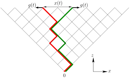
Figure 1: (Color online) Schematic diagram of the model. The strands of the DNA are shown by thick solid lines. The end monomers of the strands are pulled along the $x$ direction with a periodic force $g(t)=G\left|\sin(\omega t)\right|$. The separation between the end monomers, $x(t)$, follows the external force $g(t)$ with a lag.

The model used in this paper has been used previously in Ref. Kapri2012 to study the hysteresis in DNA unzipping by changing the pulling rate. In this model, the two strands of a homo-polymer DNA are represented by two directed self-avoiding walks on a ($d=1+1$)-dimensional square lattice. The walks starting from the origin are restricted to go towards the positive direction of the diagonal axis (z-direction) without crossing each other. The directional nature of the walks takes care of self-avoidance and the correct base pairing of DNA, i.e., the monomers that are complementary to each other are allowed to occupy the same lattice site. For each such overlap there is a gain of energy $-\epsilon$ ($\epsilon>0$). One end of the DNA is anchored at the origin and a time-dependent periodic force

$$g(t)=G\left|\sin\left(\omega t\right)\right|,$$ (1)

with angular frequency $\omega$ and amplitude $G$ acts along the transverse direction ($x$ direction) at the free end. The strands of the DNA cannot cross each other, therefore, in the negative cycle of the sine function the strands remain in the zipped state. By taking the absolute value of the sine function in Eq. (1), we have converted the negative cycles to positive, thus reducing the time period by half. Hence the angular frequency of the external force is $\omega=\pi\nu$ ($\nu$ is the linear frequency). Throughout the paper, by frequency we mean the angular frequency. The schematic diagram of the model is shown in Fig. 1.

In the limit $\omega\to 0$, i.e., the static force limit, this model can be solved exactly via a generating function and the exact transfer matrix techniques. It has been used previously to obtain the phase diagrams of the DNA unzipping Marenduzzo2001 ; Marenduzzo2002 ; Kapri2004 . For the static force case, the temperature dependent phase boundary is given by

$$g_{c}(T)=-\frac{T}{2}\ln\lambda(z_{2}),$$ (2)

where $\lambda(z)=(1-2z-\sqrt{1-4z})/(2z)$ and $z_{2}=\sqrt{1-e^{-\beta\epsilon}}-1+e^{-\beta\epsilon}$. The zero force melting takes place at a temperature $T_{m}=\epsilon/\ln(4/3)$ (for details see Ref. Kapri2012 ). In this paper we will be working at temperature $T=1$, and from Eq. (2) we get the critical force $g_{c}(1)=0.6778\dots$.

We perform Monte Carlo simulations of the model by using the METROPOLIS algorithm. The strands of the DNA undergo Rouse dynamics that consists of local corner-flip or end-flip moves Doi1986 that do not violate mutual avoidance (the self-avoidance is taken care of by the directional nature of the walks). The elementary move consists of selecting a random monomer from a strand, which itself is chosen at random, and flipping it. If the move results in overlapping of two complementary monomers, thus forming a base-pair between the strands, it is always accepted as a move. The opposite move, i.e. the unbinding of monomers, is chosen with the Boltzmann probability $\eta=\exp(-\epsilon/k_{B}T)$. If the chosen monomer is unbound, whatever remains unbound after the move is performed is always accepted. The time is measured in units of Monte Carlo Steps (MCS). One MCS consists of $2N$ flip attempts, i.e., on an average, every monomer is given a chance to flip. Throughout the simulation, the detailed balance is always satisfied. From any starting configuration, it is possible to reach any other configuration by using the above moves. Throughout this paper, without loss of generality, we have chosen $\epsilon=1$ and $k_{B}=1$.

At any given frequency $\omega$ and the force amplitude $G$, if the time $t$ is incremented by unity, the external force $g(t)$ changes, according to Eq. (1), from $0$ to a maximum value $G$ and then decreases to $0$. Between each time increment, the system is relaxed by a unit time (1MCS). Upon incrementing $t$ further, the above cycle gets repeated again and again. Before taking any measurement, the simulation is run for $2000$ cycles so that the system can reach the stationary state.

At this point, it is worthwhile to compare our model with the model of Kumar et al. Kumar2013 ; Mishra2013 ; Mishra2013jcp . In their model, a chain of length $N$, whose first $N/2$ monomers are complementary to the rest half, is anchored (at origin) from one end, and a periodic force is acting on the free end along $x-$direction. The monomers of the chain are chosen in such a manner that the $i$th monomer from the anchored end can bind only wit theh $(N-i)$th monomer of the chain, thus mimicking the base pair of the DNA. The system evolves in the presence of an external periodic force, and the distance of the end monomer from the origin, $x(t)$, is monitored as a function of time by using Langevin dynamics simulation. If $x(t)<5$ (for $N=32$) the DNA is taken to be in the zipped state, otherwise it is in the unzipped state. Their model becomes similar to ours (see Fig. 1) if, instead of first, the bead at the center of the chain is anchored, and a periodic force is applied on the first and the last monomers in opposite directions. In both models, the forcing is such that the force, averaged over a cycle, applied on the DNA is not equal to zero. Therefore, we expect that for a given amplitude $G$, both models will have similar steady states in the larger frequency limit. This is indeed the case. For lower values of $G$ (e.g., $G=0.4$ in Ref. Kumar2013 and $G=1$ in our case), the steady state is a zipped configuration, while for higher values of $G$ (e.g., $G=1$ in Ref. Kumar2013 and $G=3$ in our case), the DNA is in an unzipped state. There are, however, few differences between the two models, but that has more to do with the simulation technique. For example, in Langevin dynamics simulations, friction needs to be introduced to equilibrate the system. In contrast, Monte Carlo dynamics is dissipative by definition and brings the system to equilibrium. Even though the Langevin dynamics simulations of Kumar et al. are done in 3 dimensions, the motion of the end bead is along the direction of an externally applied force. The quantity of interest is the hysteresis traced out by the end monomer. For temperatures below the melting temperature of DNA, the fluctuations of the end bead along the transverse directions are small and hence the area of the hysteresis loop in the transverse directions is negligible. We have checked this for a self avoiding polymer in three dimensions. Therefore, our two-dimensional model captures the essential physics of dynamic transitions, and we expect values for the exponents $\alpha$ and $\beta$ similar to those obtained by Kumar et al. Kumar2013 ; Mishra2013jcp .

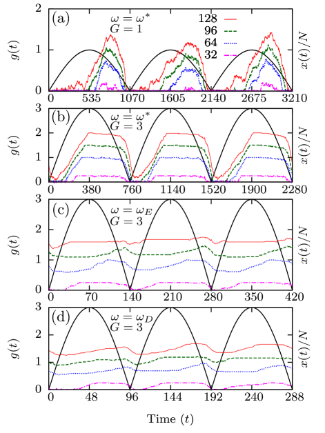
Figure 2: (Color online) (a) The time variation of the external force $g(t)$ for frequency $\omega=\omega^{*}=2.94\times 10^{-3}$ at force amplitude $G=1$. Various lines represent the scaled extension, $x(t)/N$, of different monomers for the DNA of length $N=128$. Parts (b), (c), and (d) are the same as (a) for $G=3$ for frequencies $\omega=\omega^{*}=4.2\times 10^{-3}$, $\omega=\omega_{E}=2.24\times 10^{-2}$, and $\omega=\omega_{D}=3.27\times 10^{-2}$. Here $\omega^{*}(G)$ is the frequency at which $A_{loop}$ is maximum, and $\omega_{D}$ and $\omega_{E}$ represent the frequencies marked by points $D$ and $E$, respectively, in Fig. 3(a).

We monitor the distance between the end monomers of the two strands as a function of time, $x(t)$, for various force amplitudes $G$ and frequency $\omega$. The time averaging of $x(t)$ over a complete period,

$$Q=\frac{\omega}{\pi}\oint x(t)dt,$$ (3)

may be used as a dynamical order parameter Chakrabarti1999 . Since the force is periodic in nature, we obtain the extension $x(g)$ as a function of force $g$ from the time series $x(t)$, and we average it over $10^{4}$ cycles to obtain the average extension $\langle x(g)\rangle$. If the force amplitude $G$ is not very small, and the frequency $\omega$ of the periodic force is sufficiently high to avoid equilibration of the DNA, the average extension, $\langle x(g)\rangle$, for the forward and the backward paths is not the same and we see a hysteresis loop. The area of the hysteresis loop, $A_{loop}$, defined by

$$A_{loop}=\oint\langle x(g)\rangle dg,$$ (4)

depends upon the frequency $\omega$ and the amplitude $G$ of the oscillating force and also serves as another dynamical order parameter Chakrabarti1999 . We bin the data generated according to values of $g$ by using Eq. (1). We first divide the interval $g\in[0,G]$, for both the rise and fall of the cycle, into $1000$ uniform intervals, and we obtain the value of $\langle x(g)\rangle$ at the end points of these intervals by interpolation using cubic splines of the GNU Scientific Library Galassi2009 . The area of the loop $A_{loop}$ is then evaluated numerically by using the trapezoidal rule on these intervals.

In this paper we report the behavior of $A_{loop}$ at high and low frequencies at various force amplitudes $G$. The results for the dynamical order parameter $Q$ will be published elsewhere KapriUnpub .

III Results and Discussions

In Fig. 2, we have shown the time variation of external force $g(t)$ and the scaled extension $x(t)/N$ of different monomers for the DNA of length $N=128$ at various $G$ and $\omega$ values for three consecutive cycles. This figure gives us important information that can be used to estimate the frequency $\omega^{*}(G)$ at which the loop area $A_{loop}$ is maximum. From Eq. (1), one can see that for $T=1$, the number of time steps required (say $t_{z}$) for a given frequency $\omega$ to increase $g(t)$ above the critical force $g_{c}(1)$ are approximately $\pi/4\omega$ and $\pi/12\omega$ for $G=1$ and $3$, respectively. Therefore, for this time, the DNA remains in a zipped state. The time required to unzip the DNA is given by $t_{u}\sim N$. Since the magnitude of the force continues to increase much beyond $g_{c}$, the DNA also keeps on stretching until it reaches a fully stretched configuration. This takes the time $t_{s}\sim N$. Assuming that the DNA takes the same time ($t_{u}+t_{s}$) in reaching a zipped configuration from the fully stretched unzipped state, the total time which sets the time scale of the dynamics of the DNA is

$$t_{tot}=2(t_{z}+t_{u}+t_{s})=\begin{cases}2\left(2N+{\pi}/{4\omega}\right)&\text{for}\ G=1\\ 2\left(2N+{\pi}/{12\omega}\right)&\text{for}\ G=3,\end{cases}$$ (5)

for two different force amplitudes. If $t_{tot}$ matches with the time period of the oscillating force (see Figs. 2(a) and 2(b)), we get the maximum loop area. This happens at the frequency

$$\omega=\omega^{*}(G)=\begin{cases}{\pi}/{8N}&\text{for}\ G=1\\ {5\pi}/{24N}&\text{for}\ G=3.\end{cases}$$ (6)

The values of $\omega^{*}(G)$ calculated from the above equation for various lengths of the DNA are tabulated in Table 1.

	$G=1$		$G=3$
$N$	$\omega^{*}=\frac{\pi}{8N}$	$\omega^{*}$ (OBS)	$\omega^{*}=\frac{5\pi}{24N}$	$\omega^{*}$ (OBS)	$\omega_{E}=\frac{11\pi}{12N}$	$\omega_{E}$ (OBS)	$\omega_{2}=\frac{3\pi}{2N}$	$\omega_{2}$ (OBS)
32	$1.2\times 10^{-2}$	$1.4(1)\times 10^{-2}$	$2.0\times 10^{-2}$	$1.8(6)\times 10^{-2}$	$9.0\times 10^{-2}$	$9.2(6)\times 10^{-2}$	$1.5\times 10^{-1}$	$1.3(1)\times 10^{-1}$
64	$6.1\times 10^{-3}$	$6.2(5)\times 10^{-3}$	$1.0\times 10^{-2}$	$8.4(4)\times 10^{-3}$	$4.5\times 10^{-2}$	$4.6(2)\times 10^{-2}$	$7.4\times 10^{-2}$	$6.5(3)\times 10^{-2}$
128	$3.0\times 10^{-3}$	$2.8(1)\times 10^{-3}$	$5.1\times 10^{-3}$	$4.2(1)\times 10^{-3}$	$2.25\times 10^{-2}$	$2.27(3)\times 10^{-2}$	$3.6\times 10^{-2}$	$3.2(2)\times 10^{-2}$
256	$1.5\times 10^{-3}$	$1.4(1)\times 10^{-3}$	$2.5\times 10^{-3}$	$1.9(1)\times 10^{-3}$	$1.12\times 10^{-2}$	$1.12(1)\times 10^{-2}$	$1.8\times 10^{-2}$	$1.63(2)\times 10^{-2}$
512	$7.7\times 10^{-4}$	$6.9(3)\times 10^{-4}$	$1.28\times 10^{-3}$	$9.5(3)\times 10^{-4}$	$5.6\times 10^{-3}$	$5.65(4)\times 10^{-3}$	$9.2\times 10^{-3}$	$8.1(1)\times 10^{-3}$

Table 1: Calculated and observed (OBS) frequencies for various lengths of the DNA for force amplitudes $G=1$ and $G=3$. The digits in bracket represent the uncertainity of the last decimal place.

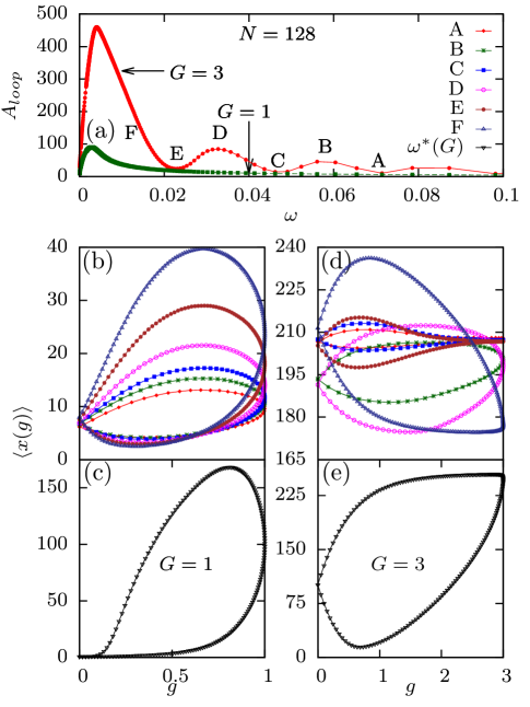
Figure 3: (Color online) (a) Area of the hysteresis loop $A_{loop}$ as a function of $\omega$ in the high frequency range for the force amplitude $G=1$ (filled squares) and $G=3$ (filled circles). The length of the DNA is $N=128$. (b) The force $g$ versus extension $\langle x(g)\rangle$ curves averaged over $10^{4}$ cycles for $G=1$ at frequencies $\omega_{A}=7.14\times 10^{-}2$, $\omega_{B}=5.61\times 10^{-2}$, $\omega_{C}=4.62\times 10^{-2}$, $\omega_{D}=3.27\times 10^{-2}$, $\omega_{E}=2.24\times 10^{-2}$, and $\omega_{F}=1.57\times 10^{-2}$, indicated, respectively, by points $A-F$ in (a). (d) Same as (b) for $G=3$. Plots (c) and (e) shows the hysteresis curves having the maximum loop area at frequencies $\omega^{*}(G=1)=2.8\times 10^{-3}$ and $\omega^{*}(G=3)=4.2\times 10^{-3}$ respectively.

In Fig. 3(a) we have plotted the area of the hysteresis loop, $A_{loop}$, as a function of frequency $\omega$, for the DNA of length $N=128$ at force amplitudes $G=1$ and $3$. The plot shows that the area of the hysteresis loop is a non monotonic function of the frequency, and its behavior depends on the amplitude of the periodic force $G$. For the equilibrium case, i.e., $\omega=0$, there is no hysteresis, resulting in a zero loop area. For very low frequencies, the force changes very slowly, the DNA gets enough time to relax to this change and it remains in equilibrium, so the loop area $A_{loop}$ is very small. Upon increasing $\omega$, the change in the force in unit time increases, and there is some lag in the response of the DNA to this change. This is depicted by an increase in the area of the hysteresis loop. The increase in $A_{loop}$ does not continue indefinitely with an increase in $\omega$. There is a frequency $\omega^{*}(G)$ ($\omega^{*}(G)\approx 2.8\times 10^{-3}$ and $4.2\times 10^{-3}$, respectively, for $G=1.0$ and $3.0$) at which $A_{loop}$ is maximum and it starts decreasing upon increasing $\omega$ above $\omega^{*}(G)$. For $G=1$, $A_{loop}$ decreases monotonically as $\omega$ increases above $\omega^{*}(G)$, whereas it shows an oscillatory component for the force amplitude $G=3$. The observed values of $\omega^{*}(G)$ obtained from the simulation are also tabulated in Table 1. These values match reasonably well with the frequencies calculated using Eq. (6).

To understand the different behavior of $A_{loop}$, we have plotted the average extension $\langle x(g)\rangle$, as a function of the applied force $g$ in Figs. 3(b)-(c) for $G=1$ and Figs. 3(d)-(e) for $G=3$, for various frequencies marked in Fig. 3(a) by capital letters ($A$ to $F$). For $G=1$, which lies slightly above the critical force, $g_{c}$, needed to unzip the DNA ($g_{c}(1)=0.6778\ldots$ from Eq. (2)), the majority of bonds of the DNA are in the zipped state (i.e., $\langle x\rangle/N<<1$) when $g=0$. (see Fig. 3(b)). When the force changes from $g=0$ to $g=G=1$ very rapidly (point $A$ in Fig. 3(a) which corresponds to $\omega=7.14\times 10^{-2}$) then the fluctuating force can open only a few base pairs of the zipped DNA at the open end and the area of the hysteresis loop is small. As $\omega$ decreases from $\omega_{A}=7.14\times 10^{-2}$ (point $A$) to $\omega_{F}=1.57\times 10^{-2}$ (point $F$), the DNA gets more time to relax, more and more base pairs become open, and the area of the hysteresis loop increases. Figure 3(c), shows the hysteresis curve having a maximum loop area at frequency $\omega^{*}(G=1)=2.8\times 10^{-3}$. Similar types of hysteresis loops are also observed for the amplitude $G=0.65$, which lies below the phase boundary. In this case, the majority of the bonds of the DNA are in the zipped state. However, at any finite temperatures, a few bonds at the end become open due to thermal fluctuations. The free ends are then dragged by the pulling force, resulting in a hysteresis loop with a small area.

The situation for the larger force amplitudes (see Fig. 3(a) for $G=3$) is however different. The force $g=G$ lies far away from the phase boundary and at this force value, the DNA is in the unzipped phase with a completely stretched conformation in the steady state. At a very high frequency $\omega_{A}=7.14\times 10^{-2}$ (point $A$), the force changes rapidly between $g=0$ and $g=G=3$ and DNA does not get enough time to respond to this change. The separation between the end monomers remains constant, resulting in a small loop area. Upon decreasing the frequency $\omega$, the DNA gets more time to relax. As a result the area of the loop starts increasing. However, it increases only up to frequency $\omega_{B}=5.61\times 10^{-2}$ (point $B$) and then decreases again till $\omega_{C}=4.62\times 10^{-2}$ (point $C$) and so on. This behavior continues up to $\omega^{*}(G=3)=4.2\times 10^{-3}$ for which we get the highest peak. Upon decreasing the frequency further the loop area decreases and becomes zero in the limit $\omega\to 0$.

The hysteresis loops (shown in Fig. 3(d) by filled diamonds, squares, and circles) at frequencies $\omega_{A}=7.14\times 10^{-2}$, $\omega_{C}=4.62\times 10^{-2}$ and $\omega_{E}=2.24\times 10^{-2}$ (points $A$, $C$ and $E$, respectively), where $A_{loop}$ has a minimum, have a peculiar shape. These loops have almost the same extension $\langle x(g)\rangle$ at the minimum ($g=0$) and the maximum ($g=G=3$) force values, and their shapes are symmetrical about the line joining them. The loops at frequencies $\omega_{B}$ and $\omega_{D}$ (point $B$ and $D$), where $A_{loop}$ has a maximum, are not symmetrical. The hysteresis curve having the maximum loop area at frequency $\omega^{*}(G=3)=4.2\times 10^{-3}$ is also shown in Fig. 3(e).

The simple analysis used at the beginning of this section to calculate the frequency $\omega^{*}(G)$ can be extended to estimate the frequency $\omega_{E}$, where the first minimum arises for the force amplitude $G=3$ (see Fig. 3(a)). It can be seen in Fig. 2(c) that for $G=3$, the 32nd monomer is in the bound state for lower values of $g(t)$. This means that a fraction, $N/4$ of the length of the DNA from the anchored end is in the zipped state. As the value of $g(t)$ increases, this bound segment of the DNA unzips. The time required to unzip this fraction is $t_{u}\sim N/4$. The kink that is generated as a result of unzipping has to travel to the free end so that the DNA can take the stretched configuration. It takes the time proportional to the length of the unbound segment of the DNA, and $t_{s}\sim 3N/4$. Therefore, the total time for this case is $t_{tot}=t_{z}+t_{u}+t_{s}\approx\pi/12\omega+N$. If this time is equal to the time period of the external force, the DNA is out of phase with the external frequency and we get a minimum, giving the frequency

$$\omega=\omega_{E}=\frac{11\pi}{12N}\quad\text{for}\ G=3,$$ (7)

at which $A_{loop}$ has the first minimum from the lower frequency side. The values of $\omega_{E}$ are also tabulated in Table 1. It matches excellently with the observed frequency. The above analysis is limited by the estimation of the fraction of zipped monomers of the DNA. This length decreases rapidly upon increasing the frequency, and its estimation becomes more and more difficult. Taking again the fraction, $N/4$ of the length of the DNA from the anchored end to be in the zipped state (see Fig.2(d)), we estimate

$$\omega=\omega_{D}\approx\frac{5\pi}{3N}\quad\text{for}\ G=3,$$ (8)

as the frequency of the second peak. This estimate has a deviation of around $20\%$ from the frequencies observed from the simulation data, which may be due to the error in the estimation of the length of the zipped segment of the DNA.

In Fig. 4, we have plotted the area of the hysteresis loop, $A_{loop}$, as a function of $\omega$ for various force amplitudes $G$ ranging from $0.65$ to $3.0$. The value $G=0.65$ lies just below the phase boundary $g_{c}(T)$ (given by Eq. (2)) for the static case ($\omega=0$), and all other values lie above it. For smaller values of $G$, the area keeps on decreasing for frequencies above $\omega^{*}(G)$ and eventually becomes zero at very high frequencies. For $G=0.65$, which lies below the phase boundary, the loop area is of the order $1$. We have scaled it by a factor of $10$ to make it visible in the plot. Therefore, in the limit $N\to\infty$, the loop area per unit length, $A_{loop}/N\to 0$ for values of $G$ that lies below the phase boundary. For higher values of $G$, however, we find that the area of the loop has an oscillatory component. It shows few more peaks of smaller heights before going to zero at very high frequencies. One such peak is shown in the inset of Fig. 4 between the frequency range $2.0\times 10^{-2}$ and $4.5\times 10^{-2}$. One can clearly see that, in this frequency range, for $G=1.0$ and $1.25$, the loop area decreases but for $G=1.5$ and higher it first increases, reaches a local maximum, and then decreases. For a given amplitude $G$, we found that the number of peaks depends on the length $N$ of the DNA. Similar oscillatory behavior is also observed in the other order parameter $Q$ KapriUnpub .

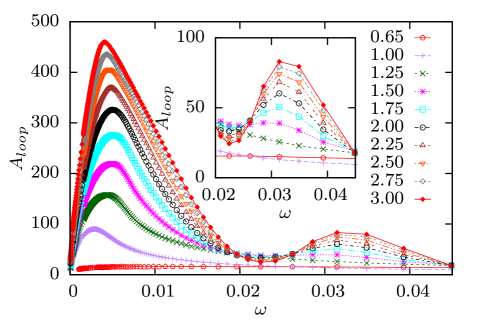
Figure 4: (Color online) Area of the hysteresis loop, $A_{loop}$, as a function of frequency $\omega$ of the periodic force for various force amplitudes $G$ for the DNA of length $N=128$. The loop area for $G=0.65$ is scaled by a factor of $10$ to make it visible in the scale. The inset shows the second peak that appears at high frequencies.

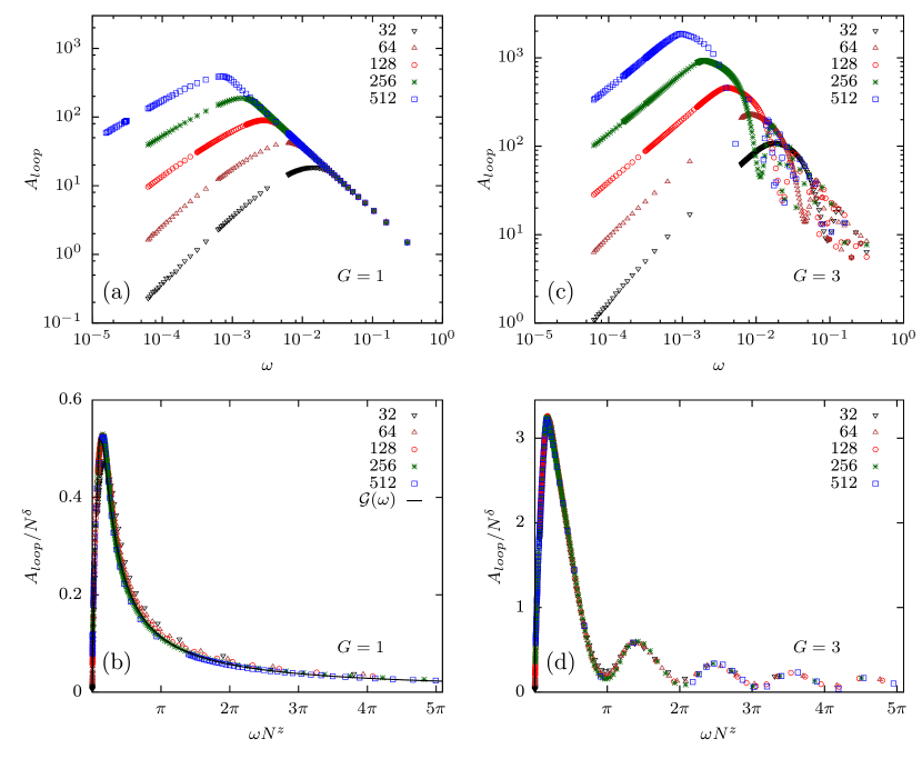
Figure 5: (Color online) Area of the hysteresis loop, $A_{loop}$, for the DNA of lengths $N=32,64,128,256,512$, as a function of frequency $\omega$ for force amplitudes (a) $G=1$, and (c) $G=3$ in log-log scale. Plots (b) and (d) represent the collapse of data shown in (a) and (c), respectively. The values of the exponents are close to $\delta=1$ and $z=1$. For $G=1$, the scaling curve $\mathcal{G}(\omega)=AG^{\alpha}\omega^{\beta}/(\omega^{1+\beta}+B^{2})$ with fitting parameters $A=0.36$ and $B=0.30$ is also plotted in (b).

In Figs. 5(a) and 5(c), we have plotted the area of the hysteresis loop, $A_{loop}$, as a function of frequency $\omega$ for the DNA of lengths $N=32$, 64, 128, 256, and 512 at force amplitudes $G=1$ and $3$, respectively, in a log-log scale. In the high frequency range the loop area decreases linearly for $G=1$ as $\omega$ increases, whereas it shows oscillatory behavior for $G=3$. The number of peaks increases as the length of the DNA increases. We explored up to the frequency $\omega=3.14\times 10^{-1}$ and found that for the DNA of length $N=32$ only one secondary peak exists, whereas for $N=512$, there are 15 peaks. Such oscillatory behavior were not not seen in earlier studies Kumar2013 ; Mishra2013jcp because they were done on short DNA (the maximum length used was only $N=32$ base pairs), with frequencies much lower than reported in this paper. In the lower frequency range, it is clearly visible that the slope of $A_{loop}$ changes as the length of the DNA increases. The above behavior shows the presence of strong finite size effects, and the exponents obtained by finite-size scaling with lengths up to $N=32$ Mishra2013jcp needs to be estimated again using longer chain lengths.

From Figs. 5(a) and 5(c), it is clear that $\omega^{*}(G)$, the frequency at which the loop area is maximum, decreases as the length of the DNA is increased. In the thermodynamic limit $N\to\infty$, from Eq. (6), we get $\omega^{*}(G)\to 0$. This suggests the scaling form for the loop area $A_{loop}$,

$$A_{loop}=N^{\delta}\mathcal{G}\left(\omega N^{z}\right),$$ (9)

where $\delta$ and $z$ are critical exponents. The exponent $z$ is the dynamic exponent as time $t\sim N^{z}$. We obtain a nice data collapse for $\delta=1.06\pm 0.05$ and $z=1.05\pm 0.03$ for $G=1$, and $\delta=1.02\pm 0.02$ and $z=1.01\pm 0.01$ for $G=3$. The data collapse for $G=1$ and $3$ are shown in Figs. 5(b) and 5(d), respectively. The scaled curve of Fig. 5(d) clearly shows an oscillatory component in the loop area for higher force amplitudes. In the following we explain the reason for getting $z=1$. For an ideal Rouse chain of length $N$, the longest relaxation time (Rouse time) $\tau_{R}\sim N^{2}$. On the time scale $t>\tau_{R}$, the motion of the chain is diffusive, i.e., the mean-square displacement is linear in time, giving $z=2$. For a constant pulling force above the phase boundary, the time $t$ required to unzip the DNA of length $N$ from a nonequilibrium zipped state to an unzipped state at equilibrium is found to be $\sim N^{2}$ Sebastian2000 ; Marenduzzo2002 . In recent years, different dynamical exponents for zipping time have been found in various DNA zipping simulations Ferrantini2011 ; Dasanna2012 . For example, an anomalous exponent of $z=1.37$ has been found in the simulations of zipping dynamics of two flexible polymers anchored at one end by Ferrantini and Carlon Ferrantini2011 . In another study, Dasanna et al. Dasanna2012 have simulated a semiflexible model of DNA that explicitly includes the bending rigidities of dsDNA segments, and they found the value $z=1.4$ for the zipping time. For the present problem, however, the frequency of the external force is such that its time period is much smaller than $\tau_{R}$. The chain never relaxes completely, and its motion is subdiffusive, i.e., the mean square displacement increases as the square root of time Rubinstein2003 . Our model also allows fluctuations in the length of the DNA. For lower values of force $g$, the DNA is in the zipped state, where it takes a zig-zag configuration. However, for higher values of $g$, the DNA is in the unzipped state with a fully stretched configuration. The average length of the DNA in the unzipped state is more than its length in the zipped state. Due to these length fluctuations, we also have longitudinal modes of the Rouse chain. For $t<\tau_{R}$, the mean squared contour length of the chain increases as the square root of time  Rubinstein2003 and therefore $z=1$. Due to the geometry of the square lattice, the change in length of the DNA by flipping a monomer (diagonal along $z-$axis) is exactly equal to the change in the separation of the end monomers (diagonal along $x-$axis). Hence the end-separation correlation function $\langle x(t)x(0)\rangle$ is exactly equal to the length correlation function and should scale as $t/N$. This is indeed found in the simulation giving $z=1$ KapriUnpub . The exponents $\delta=1$ and $z=1$ are similar to the exponents obtained in Ref. Mishra2013jcp using DNA of shorter lengths.

A Rouse chain of length $N$ has natural frequencies at $(2p-1)\pi/2N$, where $p=1,2,\ldots$ are integers. When this frequency matches with the frequency $\omega$ of the externally applied periodic force, we get a resonance. From Fig. 5(d), one can see that for $G=3$, the location of maxima (minima) is situated when the scaled frequency $\omega N$ is an odd (even) integral multiple of $\pi/2$. Therefore, the length dependent frequency $\omega_{p}$ of these maxima (minima) is given by

$$\omega_{p}=\begin{cases}{(2p-1)\pi}/{2N}&\text{(maxima)}\cr{p\pi}/{N}&\text{(minima)},\end{cases}$$ (10)

where $p=1,2,\ldots$ are integers. From the above expression, the first peak, which corresponds to the maximum loop area, has a frequency $2.5$ times higher than that predicted by Eq. (6). However, the frequencies of the higher peaks and valleys that are estimated by Eq. (10) are quite close to those observed in the simulation. This is because these modes, as opposed to the first mode, get completely relaxed within the time period of the applied force. The values of the second mode $\omega_{2}$ for various $N$ are also tabulated in Table 1. These matches extremely well with the observed frequencies.

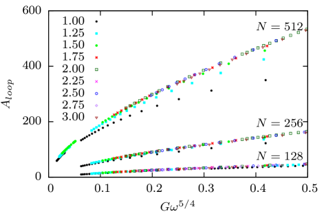
Figure 6: (Color online) Area of the hysteresis loop $A_{loop}$ versus $G\omega^{5/4}$ for the DNA of lengths $N=128$, 256, and 512 at low frequencies for various $G$ values.

In Fig. 6, we have plotted the area of the hysteresis loop, $A_{loop}$, as a function of $G^{\alpha}\omega^{\beta}$ in the low frequency range for the DNA of lengths $N=128$, 256, and 512 at various force amplitudes $G$. A good data collapse is obtained for the values $\alpha=1.0\pm 0.05$ and $\beta=1.25\pm 0.05$. The values of $\alpha$ and $\beta$ differ considerably with previously obtained values $\alpha=\beta=1/2$ Kumar2013 ; Mishra2013jcp . We believe that the lower values of exponents are due to the shorter chain lengths used in their simulations.

The scaling function $\mathcal{G}(\omega)$ can be obtained by observing that at low frequencies ($\omega\to 0$), for large $N$, the $A_{loop}$ scales as $G^{\alpha}\omega^{\beta}$, while at very high frequencies ($\omega\to\infty$), from Eq. (9), we see $A_{loop}\sim 1/\omega$. For smaller $G$ values the steady state is a zipped configuration, and the area of the loop decreases monotonically for $\omega$ above $\omega^{*}(G)$ (e.g., $G=1$). For such cases, the scaling function $\mathcal{G}(\omega)$ that satisfies the above requirements has the form

$$\mathcal{G}(\omega)=\frac{AG^{\alpha}\omega^{\beta}}{\omega^{1+\beta}+B^{2}},$$ (11)

with $A$ and $B$ as fitting parameters. The scaling function for $G=1$, with parameters $A=0.36$ and $B=0.30$, obtained by data fitting, is plotted in Fig. 5(b). For moderate force amplitudes (say $G=1.25$), we found that the above scaling function is still valid with parameters $A=0.78$ and $B=0.39$.

For higher force amplitudes, the steady state is a completely stretched unzipped state, and the loop area has an oscillatory component above $\omega^{*}(G)$. For such cases, the above form is not suitable as the scaling function.

IV Conclusions

In this paper we have studied the hysteresis in unzipping of a dsDNA by a periodic force with frequency $\omega$ and amplitude $G$ for chains up to lengths $N=512$ by using Monte Carlo simulations. The behavior of the loop area depends on the force amplitudes. We find that for lower $G$ values, the steady state of the DNA is a zipped configuration. The area of the loop shows only one peak at $\omega^{*}(G)$, and for frequencies above $\omega^{*}(G)$, it decreases monotonically. However, for higher force amplitudes, the steady state is an unzipped state and the area of the loop shows multiple peaks. We gave a simple analysis that could estimate $\omega^{*}(G)$, the frequency at which the maximum loop area is observed, and the frequencies of other peaks that appear for higher force amplitudes. We also explored the behavior of the hysteresis loop area for a wide range of frequencies for both lower and higher values of force amplitudes $G$ using the finite-size scaling. We found that the loop area scales as $1/\omega$ in the high-frequency range, whereas it scales as $G^{\alpha}\omega^{\beta}$ with exponents $\alpha=1$ and $\beta=5/4$ in the low-frequency regime. These exponents are found to be different from the values obtained by Kumar et al. Kumar2013 ; Mishra2013jcp . We believe that the different values of exponents $\alpha$ and $\beta$ are due to the shorter chain lengths used in their studies. It would be interesting to study longer chain lengths using Langevin dynamics simulations to confirm the above results. The other interesting direction would be to include the bending rigidity of dsDNA that has been ignored in this paper and study its influence on the dynamic exponents as a function of chain lengths. In fact, for chains of the order of persistence length of the DNA, the bending rigidity could play an important role and the dynamic exponents may be different than reported in this paper. However, in the thermodynamic limit, the bending rigidity would not be relevant and we believe that the exponents of the flexible chain will be recovered. This, however, will require further investigations.

References

- (1) F. Ritort, J Phys Condens Matter 18, R531 (2006).
- (2) S. M. Bhattacharjee, J. Phys. A 33, L423 (2000).
- (3) D. K. Lubensky and D. R. Nelson, Phys. Rev. Lett. 85, 1572 (2000).
- (4) K. L. Sebastian, Phys. Rev. E 62, 1128 (2000).
- (5) U. Bockelmann et al., Biophys. J. 82, 1537 (2002).
- (6) C. Danilowicz, Y. Kafri, R. S. Conroy, V. W. Coljee, J. Weeks, M. Prentiss, Phys. Rev. Lett. 93, 078101 (2004).
- (7) J. D. Watson et al., Molecular Biology of the Gene, 5th ed. (Pearson/Benjamin Cummings, Singapore, 2003).
- (8) D. Marenduzzo, A. Trovato, and A. Maritan, Phys. Rev. E 64, 031901 (2001).
- (9) D. Marenduzzo, S. M. Bhattacharjee, A. Maritan, E. Orlandini and F. Seno, Phys. Rev. Lett., 88, 028102 (2001).
- (10) R. Kapri, S. M. Bhattacharjee, and F. Seno, Phys. Rev. Lett. 93, 248102 (2004).
- (11) R. Kapri and S. M. Bhattacharjee, J. Phys.: Condensed Matter, 18, 215 (2006).
- (12) R. Kapri and S. M. Bhattacharjee, Phys. Rev. Lett. 98, 098101 (2007).
- (13) R. Kapri and S. M. Bhattacharjee, EPL 83, 68002 (2008).
- (14) R. Kapri, J. Chem. Phys. 130, 145105 (2009).
- (15) S. Kumar and M. S. Li, Phys. Rep. 486, 1 (2010).
- (16) K. Hatch, C. Danilowicz, V. Coljee, and M. Prentiss, Phys. Rev. E 75, 051908 (2007).
- (17) R. W. Friddle, P. Podsiadlo, A. B. Artyukhin, and A. Noy, J. Phys. Chem. C 112, 4986 (2008).
- (18) Z. Tshiprut and M. Urbakh, J. Chem. Phys. 130, 084703 (2009).
- (19) P. T. X. Li, C. Bustamante, and I. Tinoco, Proc. Natl. Acad. Sci. (U.S.A.) 104, 7039 (2007).
- (20) G. Mishra, P. Sadhukhan, S. M. Bhattacharjee, and S. Kumar, Phys. Rev. E 87, 022718 (2013).
- (21) S. Kumar and G. Mishra, Phys. Rev. Lett. 110, 258102 (2013).
- (22) B. K. Chakrabarti and M. Acharyya, Rev. Mod. Phys. 71, 847 (1999).
- (23) R. K. Mishra, G. Mishra, D. Giri, and S. Kumar, J. Chem. Phys. 138, 244905 (2013).
- (24) R. Kapri, Phys. Rev. E 86, 041906 (2012).
- (25) M. Doi and S. F. Edwards, The Theory of Polymer Dynamics (Oxford University Press, New York, 1986).
- (26) M. Galassi et al., Gnu Scientific Library Reference Manual, 3rd ed. (Network Theory Ltd., Bristol, UK, 2009).
- (27) R. Kapri, unpublished.
- (28) A. Ferrantini and E. Carlon, J. Stat. Mech., P02020 (2011).
- (29) A. K. Dasanna, N. Destainville, J. Palmeri and M. Manghi, EPL, 98, 38002 (2012).
- (30) M. Rubinstein and R. H. Colby, Polymer Physics, 1st ed. (Oxford University Press, Oxford, 2003).