Two conjectures about spectral density of diluted sparse Bernoulli random matrices

Abstract

We consider the ensemble of $N\times N$ ($N\gg 1$) symmetric random matrices with the bimodal independent distribution of matrix elements: each element could be either ”1” with the probability $p$, or ”0” otherwise. We pay attention to the ”diluted” sparse regime, taking $p=1/N+\varepsilon$, where $0<\varepsilon\ll 1/N$. In this limit the eigenvalue density, $\rho(\lambda)$, is essentially singular, consisting of a hierarchical ultrametric set of peaks. We provide two conjectures concerning the structure of $\rho(\lambda)$: (i) we propose an equation for the position of sequential (in heights) peaks, and (ii) we give an expression for the shape of an outbound enveloping curve. We point out some similarities of $\rho(\lambda)$ with the shapes constructed on the basis of the Dedekind modular $\eta$-function.

I Preliminaries and conjectures

The Bernoulli matrix model considered in this letter, is defined as follows. Take a large $N\times N$ symmetric matrix $A$ ($N\gg 1$) with the matrix elements, $a_{ij}=a_{ji}$, independent identically distributed random variables, equal to ”1” with probability $p$ for any $i\neq j$, and to ”0” otherwise. This defines the uniform distribution on the entries $a_{ij}$:

$${\rm Prob}(a_{ij})=p\delta(a_{ij}-1)+(1-p)\delta(a_{ij}),$$ (1)

where $\delta$ is the Kronecker symbol: $\delta(x)=1$ for $x=0$, and $\delta(x)=0$ otherwise. The matrix $A$ can be regarded as an adjacency matrix of a random Erdös-Rényi graph without self-connections. Obviously, all the eigenvalues, $\lambda_{n}$ ($n=1,...N$) of the matrix $A$ are real.

Let $\rho(\lambda)$ be the eigenvalue density in the ensemble of $A$. For $N\gg 1$ the limiting shape of $rho(\lambda)$ is known in various cases. If $p$ is large enough (of order of unity), then for $N\gg 1$ the function $\rho(\lambda)$ tends to the Wigner semicircle law, $\sqrt{4N-\lambda^{2}}$, typical for the Gaussian matrix ensembles. For $p=c/N$ ($c>1$), the matrix $A$ is sparse and the density $\rho(\lambda)$ in the ensemble of sparse matrices has singularities at finite values of $c$ rod1 ; rod2 ; fyod . At $c=1$ one has in average of order of one nonzero element in any row of $A$ and therefore below $c=1$ the entire matrix becomes a collection of almost disjoint elements. This results in the trivial spectral density, $\rho(\lambda)=\delta(\lambda)$, in the ensemble of $A$. In the works evan ; bauer ; sem ; kuch the behavior of the spectral density, $\rho(\lambda)$, has been analyzed in the limit when $c$ tends to unity. It has been pointed out that the function $\rho(\lambda)$ becomes more and more singular as $c$ approaches 1. Slightly above 1, the typical subgraphs of the random matrix $A$, are basically random linear chains or disjoint trees and the eigenvalues of the entire matrix $A$ are given by corresponding characteristic polynomials of these simple graphs. Few typical samples of randomly generated by Mathematica $200\times 200$ matrices $A$ at $p=0.00502=1/N+2\times 10^{-5}$ (i.e. for $c=1.004$) are shown in the Fig.1. Note the essential fraction of linear subgraphs. The trees with loops appear rarely.

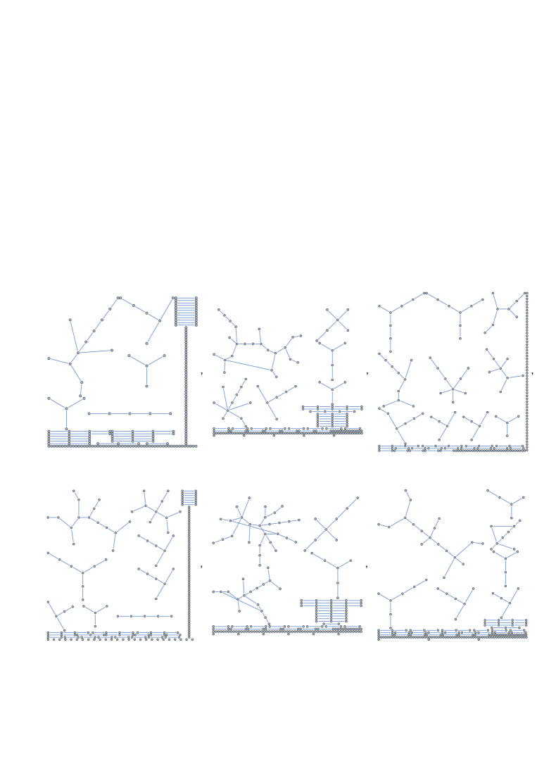
Figure 1: Few typical samples of collections of graphs of randomly generated $200\times 200$ adjacency Bernoulli matrix $A$ at $p=0.00502=1/N+2\times 10^{-5}$.

The eigenvalues contributing to the spectrum of $A$, for example, from a 3-star graph, are obtained from the following equation

$$\det\left(\begin{array}[]{cccc}-\lambda&1&0&0\\ 1&-\lambda&1&1\\ 0&1&-\lambda&0\\ 0&1&0&-\lambda\end{array}\right)=0$$ (2)

whose solution is $\lambda=\{0,0,\sqrt{3},\sqrt{3}\}$.

The whole spectrum of a symmetric matrix $A$ consists of singular peaks, located at $\lambda_{i}$ ($i=1,..N$), while the heights of peaks are the multiplicities of $\lambda_{i}$. The singular spectral density, $\rho(\lambda)$, for an ensemble of 1000 random symmetric matrices $A$, each of size $200\times 200$ and generated with the probability $p=0.00502$, is shown in the Fig.2. One can note that the spectrum possess the ultrametric hierarchical structure. In this letter we conjecture some statistical properties of the spectral density, $\rho(\lambda)$, of ensemble of sparse random symmetric matrices in the limit $p=1/N+\varepsilon$, where $0<\varepsilon\ll 1/N$.

Figure 2: Ultrametric hierarchical structure of a spectral density, $\rho(\lambda)$, for ensemble of 1000 symmetric random $200\times 200$ Bernoulli matrices, generated at $p=0.00502=1/N+2\times 10^{-5}$.

The singular spectral density depicted in the Fig.2 is compared in the Fig.3 with the function $g(\lambda)$, defined as follows

$$g(\lambda)=\left[-\ln f\left(\frac{1}{\pi}\arccos\frac{\lambda}{2}\Big{|}y\right)\right]^{2}\qquad(0<y\ll 1)$$ (3)

where

$$f(x|y)=A|\eta(x+iy)|\qquad(-2<x<2,\;y>0)$$ (4)

is the Dedekind $\eta$-function ($A$ is some normalization constant). Since the spectral density $\rho(\lambda)$ is symmetric, later on we inspect only the part $\lambda\geq 0$.

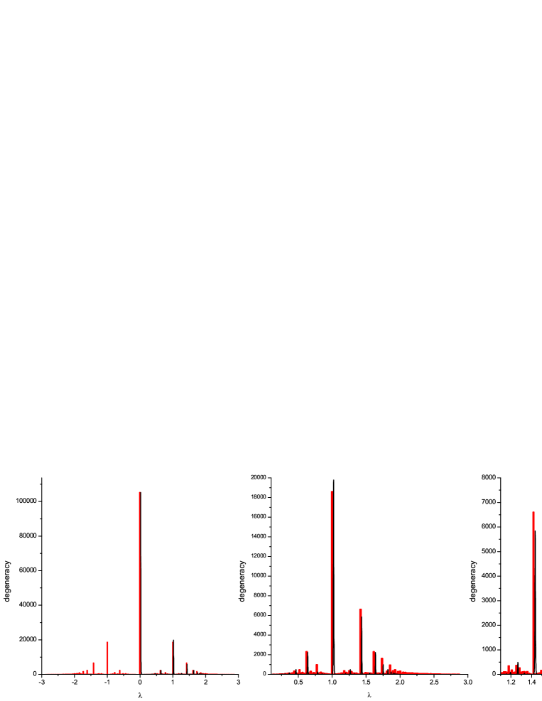
Figure 3: Numerical data, shown in red is as in the Fig.2 and the analytic curve, shown in black is given by (3)–(4). The small shift in $\Delta\lambda=+0.02$ between red and black curves is specially inserted by hands to make data distinguishable.

As one sees from the Fig.3 the correspondence between our numerical eigenvalue counting for random symmetric sparse Bernoulli matrices $A$ with the function $g(x)$, defined in (3)–(4), is good in the bulk (we have specially introduced the small shift in $\Delta\lambda=0.02$ between numerical data and analytic expression to make them distinguishable). One also sees that the tails of the spectral density $\rho(\lambda)$ are poorly reproduced by the guessed function. Apparently this is due to the contribution to $\rho(\lambda)$ from complex tree-like graphs as well as from non-tree-like graphs, which are present in the ensemble for given $\varepsilon$ as one can see from the list of graphs in the Fig.1.

Below we formulate two conjectures. In the first we propose an equation for the position of sequential (in heights) peaks, while in the second we give an expression for the shape of an outbound enveloping curve for the spectral density. These conjectures are based on a combination of rigorous results concerning the spectra of tree-like graphs obtained in rojo1 ; rojo2 ; rojo3 ; sen , with some observations of ultrametric properties of a Dedekind modular $\eta$-function.

Conjecture 1. Any eigenvalue, $\lambda_{i}$, contributing to the spectral density, $\rho(\lambda)$ for $p=1/N+\varepsilon$ ($N\gg 1$ and $\varepsilon\to 0$), can be uniquely associated with the rational number, $\displaystyle\frac{p_{i}}{q_{i}}$, where $p_{i}$ and $q_{i}$ are coprimes, as follows

$$\lambda_{i}=-2\sqrt{d}\cos\frac{\pi p_{i}}{q_{i}}$$ (5)

where $d$ is the maximal vertex degree of trees. In diluted sparse regime one has mainly $d=1$ (linear chains) or $d=2$ (star-like graphs).

The outbound enveloping peaks, $\lambda_{1},\lambda_{2},...$ (see Fig.2) are located at

$$\lambda_{m}=2\cos\frac{\pi}{m+1}\qquad(m=1,2,...)$$ (6)

Conjecture 2. The function $f(\lambda)=\rho^{1/\nu}(\lambda)$ for $\nu=4$ brings any subsequence of monotonically increasing (or monotonically decreasing) peaks into a linear form $f(\lambda)=a+b\lambda$, where $a$ and $b$ are subsequence-dependent constants. In particular, under such a transformation, the spectral density (and the outbound enveloping shape as well) acquires the triangular shape (see the Fig.6). Thus, the outbound enveloping curve for the spectral density, $\rho(\lambda)$, has the following parametric representation ($0\leq\lambda\leq 2$):

$$\rho(\lambda)=c\,(2-\lambda)^{\nu}=\left(2-2\cos\frac{\pi}{m+1}\right)^{\nu}\qquad(m=1,2,...)$$ (7)

where $c$ is some constant. The comments concerning this conjecture are given in the Section II.2.

II Hints beyond the conjectures

The positions of peaks in the spectrum can be found by using the results of the works rojo2 ; rojo3 , where the spectral properties of trees have been investigated. In particular, it has been found in rojo3 that the spectrum of a regular tree-like graph is defined by the eigenvalues of the three-diagonal symmetric matrix. The Conjecture 1 is based on the supposition that the set of outbound peaks in the eigenvalue density $\rho(\lambda)$ is the set of maximal eigenvalues $\{\lambda_{\rm max}^{(1)},\,\lambda_{\rm max}^{(2)},...\}$, where $\displaystyle\lambda_{\rm max}^{(m)}=2\cos\frac{\pi}{m+1}$ is the maximal eigenvalue of an $m$-vertex linear subchain. Examining the Fig.2 one can see that the spectral density $\rho(\lambda)$ extends beyond the value $\lambda=2$ which is the terminal eigenvalue for linear chains. This means that near the tails of the distribution the tree-like graphs and graphs with loops become dominant – see the Section II.2 for more discussion. Apparently these subgraphs cannot be eliminated by decreasing $\varepsilon$.

The Conjecture 2 is more involved and is motivated by some similarities between the spectral density $\rho(\lambda)$ and the ultrametric structure of ”continuous trees” isometrically embedded in hyperbolic domains nech1 . Below we summarize some facts concerning the ”isometric continuous trees”.

II.1 Ultrametric structure of isometric Cayley trees

Any regular Cayley tree, as an exponentially growing structure, cannot be isometrically embedded in an Euclidean plane. The embedding of a Cayley tree ${\cal C}$ into the metric space is called ”isometric” if ${\cal C}$ covers that space, preserving all angles and distances. The Cayley tree ${\cal C}$ isometrically covers the surface of constant negative curvature (the Lobachevsky plane) ${\cal H}$. One of possible representations of ${\cal H}$, known as a Poincaré model, is the upper half-plane ${\rm Im}\,z>0$ of the complex plane $z=x+iy$ endowed with the metric $ds^{2}=\frac{dx^{2}+dy^{2}}{y^{2}}$ of constant negative curvature. In nech1 we have constructed the ”continuous” analog of the standard 3-branching Cayley tree by means of special (modular) functions and have analyzed the structure of the barriers separating the neighboring valleys. In particular, we have shown that due to specific properties of modular functions these barriers are ultrametrically organized. The main ingredient of our construction was the function $f(z)$ defined as follows:

$$\tilde{f}(z)=C^{-1}\,|\eta(z)|\,({\rm Im}\,z)^{1/4}$$ (8)

where $\eta(z)$ is the Dedekind $\eta$-function (see, for instance chand )

$$\eta(z)=e^{\pi iz/12}\prod_{k=0}^{\infty}(1-e^{2\pi ikz});\qquad{\rm Im}\,z>0$$ (9)

The normalization constant $C=\left|\eta\left(\frac{1}{2}+i\frac{\sqrt{3}}{2}\right)\right|\,\left(\frac{\sqrt{3}}{2}\right)^{1/4}=0.77230184...$ is chosen to fix the maximal value of the function $\tilde{f}(z)$ equal to 1: $0<\tilde{f}(z)\leq 1$ for any $z$ in the upper half-plane ${\rm Im}\,z>0$. The function $\tilde{f}(z)$ has the following property: all the solutions of the equation $\tilde{f}(z)-1=0$ define all the coordinates of the 3-branching Cayley tree isometrically embedded into the upper half-plane ${\cal H}(z|{\rm Im}\,z>0)$. The corresponding Cayley tree and the density plot of the function $\tilde{f}(z)$ in the region $\{0\leq{\rm Re}\,z\leq 1,\;0.04\leq{\rm Im}\,z\leq 1.4\}$ is shown in fig.4. It is noteworthy that the function $Z(z)=\left[C\,\tilde{f}(z)\right]^{-2}$ is invariant with respect to the action of the modular group $PSL(2,\mathbb{Z})$, namely, $Z(z)=Z(z+1)$ and $Z(z)=Z\left(-\frac{1}{z}\right)$. The 3D relief of the function $f(z)$ is shown in figure 4(right).

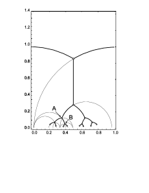
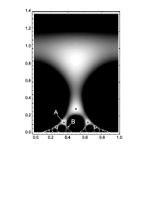
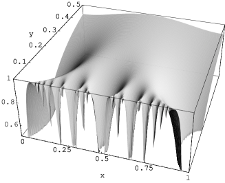
Figure 4: Left: 3-branching Cayley tree isometrically embedded in Poincaré hyperbolic upper half-plane ${\cal H}$. Center: Density plot of the function $\tilde{f}(z)$ (see the text) in the rectangle $\{0\leq{\rm Re}\,z\leq 1,\;0.01\leq{\rm Im}\,z\leq 1.4\}$. Right: Relief of the function $\tilde{f}(z)$ in the rectangle $\{0\leq{\rm Re}\,z\leq 1,\;0.04\leq{\rm Im}\,z\leq 1.4\}$.

The ”continuous tree-like structure” of hills separated by the valleys is clearly seen in the Fig.4. Consider now the function

$$v(x|y)=-\ln\tilde{f}(x|y);\qquad x={\rm Re}\,z;\;y={\rm Im}\,z$$ (10)

The typical shape of the function $v(x|y)$, shown in the figure Fig.5(left), demonstrates the ultrametric organization of the barriers separating the valleys. In the figure Fig.5(right) we have drawn the relief of the function $u(x)=v^{1/2}(x)$. Such a transformation highlights the ”linearity” of growth of sequentially increasing and decreasing barriers. This fact can be exactly proved using the algebraic properties of the Dedekind $\eta$-function (see the Appendix 1).

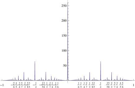
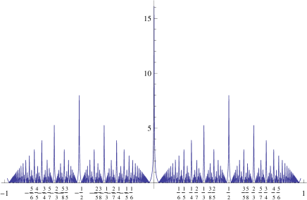
Figure 5: Typical shape of the functions $v(x)=v(x|y=0.001)$ (left) and $\sqrt{v(x)}=\sqrt{v(x|y=0.001)}$ (right).

The function $v(x)=-\ln\tilde{f}(x)$, defined on the interval $0<x<1$, has the properties borrowed from the structure of the underlying modular group $PSL(2,\mathbb{Z})$ acting in the half–plane ${\cal H}(z|y>0)$ magnus ; beardon . In particular: (i) the local maxima of the function $v(x)$ are located at the rational points; (ii) the highest barrier on a given interval $\Delta x=[x_{1},x_{2}]$ is located at a rational point $\frac{p}{q}$ with the lowest denominator $q$. On a given interval $\Delta x=[x_{1},x_{2}]$ there is only one such point. The locations of the barriers with the consecutive heights on the interval $\Delta x$ are organized according to the group operation:

$$\frac{p_{1}}{q_{1}}\oplus\frac{p_{2}}{q_{2}}=\frac{p_{1}+p_{2}}{q_{1}+q_{2}}$$ (11)

The Fig.5 clarify this statement. The highest barriers on the interval $0\leq x\leq 1$ are located at the points $x_{0}=0$ and $x_{1}=1$. Rewriting $0$ and $1$ correspondingly as $\frac{0}{1}$ and $\frac{1}{1}$ we can find the point $x_{2}$ of location of the barrier with the next maximal hight. Namely, $x_{2}=\frac{0}{1}\oplus\frac{1}{1}=\frac{0+1}{1+1}=\frac{1}{2}$. Continuing this construction we arrive at the hierarchical structure of barriers located at rational points organized in the Farey sequence.

II.2 Back to the spectral density of diluted sparse matrices

Now we are in position to give a hint why the function $g(\lambda)$ has appeared in (3)–(4). The argument, $\frac{1}{\pi}\arccos\frac{\lambda}{2}$, of the function $f(...)$ in (3) is just the inverted expression of (5). This expression projects back the eigenvalues $\lambda_{i}$ to the rational numbers $\displaystyle\frac{p_{i}}{q_{i}}$.

We have noted that the spectral density $\rho(\lambda)$ looks pretty much similar as the function $v^{2}(\lambda|y)$ taken at some fixed $0<y\ll 1$. Just this comparison is plotted in the Fig.3. The appearance of the exponent $\nu=4$ in (7) is the consequence of the guess (3). Namely, since $g(\lambda)\sim v^{2}(\lambda)$ and the function $v^{1/2}(\lambda)$ brings the Dedekind relief to the linear shape, we conclude that the function $g^{1/4}(\lambda)$ makes the shape of the transformed spectral density $\rho^{1/4}(\lambda)$ also linear – see the Fig.6. The deviation from the linearity at the tails of the Dedekind analytic disappear in the limit $y\to 0$ as one can see from the (21).

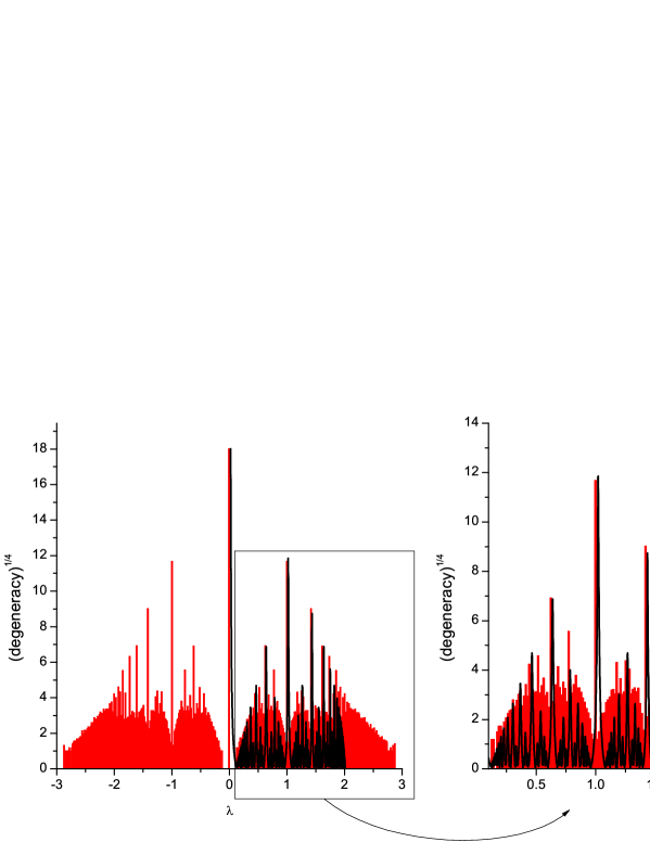
Figure 6: The same distributions as in Fig.3, but the plotted functions are: $\rho^{1/4}(\lambda)$ (red) and $g^{1/4}(\lambda)$ (black).

The discrepancy between tails of the functions $\rho(\lambda)$ and $g(\lambda)$ are due to essential contributions from large tree-like graphs, as well as from non-tree-like graphs in the sparse matrix ensemble. According to rojo3 , the largest eigenvalue of the tree-like graph can be roughly estimated as $\lambda_{\rm max}\leq 2\sqrt{d}$ where $d$ is the maximal vertex degree of a tree. In the bulk of the spectrum the contribution from the linear chain-like graphs (i.e. graphs with $d=2$) dominate, while at the edge of the spectrum the contribution from tree-like graphs with $d>2$ become essential.

Note however that heavy tails of the function $\rho^{1/4}(\lambda)$ beyond the terminal value $|\lambda|=2$ for chain-like graphs, also demonstrate linear behavior (however with a slope different from the slop in a bulk).

III Discussion

In this letter we have conjectured that the spectral density, $\rho(\lambda)$ of an ensemble of ”diluted” random symmetric sparse Bernoulli matrices demonstrates in the bulk the structure which can be roughly reproduced using the construction which involves the Dedekind modular $\eta$-function.

Yet we have not any proof of the connection between $\rho(\lambda)$ and the Dedekind $\eta$-function, however this similarity seems not occasional. Rephrasing the question of M. Kac kac as ”Can one hear the shape of a tree?”, we expect that some information about the spatial structure of a tree is encoded in its spectrum. The Weyl’s conjecture (which allows one to estimate the size and the area of the surface by the total number of eigenvalues) applied to trees, does not help much because the number of eigenvalues trivially coincides with the size of the adjacency matrix of a tree, and the area of a tree is indistinguishable from the volume (both are the number of a tree vertices). Nevertheless one sees that non-isomorphic trees have different sets of eigenvalues. What is the spectral density, $\rho(\lambda,k)$ of ensemble of all trees of a given number of vertices, $N$, and a fixed maximal backbone length, $k$? Despite some important results are obtained in rojo3 for particular tree-like graphs, the full answer to this question is still not known.

On the other side, the Dedekind function has appeared in some counting problems in hyperbolic domains related to so-called ”arithmetic chaos” considered by M. Gutzwiller and B. Mandelbrot gut . In particular they found the connection of the arithmetic function $\beta(\xi)$ which maps some number $\xi\in[0,1]$, written as a continued fraction expansion

$$\frac{1}{n_{1}+\displaystyle\frac{1}{n_{2}+\ldots}}$$ (12)

to the real number $\beta$, whose binary expansion is made by the sequence of $n_{1}-1$ times 0, followed by $n_{2}$ times 1, then $n_{3}$ times 0, and so on. In the work series C. Series pointed out the that the continued fraction expansion (12) is related to the following counting problem in the hyperbolic upper half-plane ${\cal H}(z|{\rm Im}\,z>0)$ – see Fig.4. Take the root point of the Cayley tree isometrically embedded in ${\cal H}$ and compute how many vertices (images) of the root point lie in the interval $[0,\xi]$. Therefore $\beta(\xi)$ is proportional to a fractal ”invariant measure” (i.e. to the number of vertices lying in the interval $[0,\xi]$). The counting of vertices, whose real part lie in $[0,\xi]$, is equivalent to counting the number of maxima of the function $|\eta(x+i0^{+})|$ in the same interval.

To summarize, let us emphasize that apparently the question considered in this letter lies at the edge of the spectral theory of tree-like graphs and the ”arithmetic chaos” dealing with isometric embedding of these graphs into the hyperbolic domains. It seems that the near future will show if our guess is correct or not.

I would like to thank Eugene Bogomolny for providing me references on spectral structure of tree-like graphs and to Olga Valba for useful discussions.

Appendix A ”Shape linearity” of the relief $u(x)=\sqrt{-\ln f(x)}$.

Let the function $f(z)$ for ${\rm Im}\,z>0$ be:

$$f(z)=\left|\eta(z)\right|\left({\rm Im}\,z\right)^{1/4}$$ (13)

where

$$\eta(z)=e^{\pi iz/12}\prod_{k=1}^{\infty}(1-e^{2\pi ikz});\quad{\rm Im}\,z>0$$ (14)

is the Dedekind $\eta$–function.

The following duality relation is valid for $f(z)$:

$$f\left(\frac{p}{q}+iy\right)=f\left(\frac{s}{q}+\frac{i}{q^{2}y}\right)$$ (15)

if and only if $p$ and $q$ are coprime, $s=(1+qr)/p$ and $r$ are integers.

Using (15) we can obtain the asymptotics of $\eta(z)$ when ${\rm Im}\,z\to 0^{+}$. Take into account the relation of Dedekind $\eta$–function with Jacobi elliptic functions:

$$\vartheta_{1}^{\prime}(0,e^{\pi iz})=\eta^{3}(z)$$ (16)

where

$$\vartheta_{1}^{\prime}(0,e^{\pi iz})\equiv\frac{d\vartheta_{1}(u,e^{\pi iz})}{du}\bigg{|}_{u=0}=e^{\pi iz/4}\sum_{n=0}^{\infty}(-1)^{n}(2n+1)e^{\pi in(n+1)z}$$ (17)

Rewrite (15) as follows:

$$\left|\eta\left(\frac{p}{q}+iy\right)\right|=\frac{1}{(qy)^{1/2}}\left|\eta\left(\frac{s}{q}+\frac{i}{q^{2}y}\right)\right|$$ (18)

Applying (16)–(17) to the r.h.s of (18), we get:

$$\left|\eta\left(\frac{p}{q}+iy\right)\right|=\frac{1}{(qy)^{1/2}}\left|e^{\frac{\pi}{4}i\left(\frac{s}{q}+\frac{i}{q^{2}y}\right)}\sum_{n=0}^{\infty}(-1)^{n}(2n+1)e^{\pi in(n+1)\left(\frac{s}{q}+\frac{i}{q^{2}y}\right)}\right|^{1/3}$$ (19)

Eq.(19) enables us to extract the asymptotics of $\eta(z)$ at ${\rm Im}\,z\to 0^{+}$:

$$\left|\eta\left(\frac{p}{q}+iy\right)\right|\Bigg{|}_{y\to 0^{+}}=\frac{1}{(qy)^{1/2}}e^{-\pi/(12q^{2}y)}$$ (20)

Thus,

$$\sqrt{-\ln\left|\eta\left(\frac{p}{q}+iy\right)\right|}\Bigg{|}_{y\to 0^{+}}=\frac{1}{q}\sqrt{\frac{\pi}{12y}}+\frac{1}{4}\left(\ln q+\ln y\right)$$ (21)

Denoting $\frac{1}{q}\equiv x$, we see from (21) the dominant contribution from the linear term in $x$ as $y\to 0^{+}$ on the ”coprime subsequences”.

References

- (1) G.J. Rodgers and A.J. Bray, Density of states of a sparse random matrix, Phys. Rev. B 37 3557 (1988)
- (2) T. Rogers, I.P. Castillo, R. Kühn, and K. Takeda, Cavity approach to the spectral density of sparse symmetric random matrices, Phys. Rev. E 78, 031116 (2008)
- (3) Y.V. Fyodorov and A.D. Mirlin, On the density of states of sparse random matrices, J. Phys. A: Math. Gen. 24 2219 (1991)
- (4) S.N. Evangelou and E.N. Economou, Spectral density singularities, level statistics, and localization in a sparse random matrix ensemble, Phys. Rev. Lett. 68, 361 (1992)
- (5) M. Bauer, O. Golinelli, Random Incidence Matrices: Moments of the Spectral Density, J. Stat. Phys. 103 301 (2001)
- (6) G. Semerjian and L.F Cugliandolo, Sparse random matrices: the eigenvalue spectrum revisited, J. Phys. A: Math. Gen. 35 4837 (2002)
- (7) R. Kühn, Spectra of sparse random matrices, J. Phys. A: Math. Theor. 41 295002 (2008)
- (8) O. Rojo and R. Soto, The spectra of the adjacency matrix and Laplacian matrix for some balanced trees, Linear Algebra and its Applications 403 97 (2005)
- (9) O. Rojo and M. Robbiano, On the spectra of some weighted rooted trees and applications, Linear Algebra and its Applications 420 310 (2007)
- (10) O. Rojo and M. Robbiano, An explicit formula for eigenvalues of Bethe trees and upper bounds on the largest eigenvalue of any tree, Linear Algebra and its Applications 427 138 (2007)
- (11) S. Bhamidi, S.N. Evans, and A. Sen, Spectra of large random trees, J. Theor. Prob. 25 613 (2012)
- (12) S.Nechaev and O.Vasilyev, Metric structure of ultrametric spaces, J. Phys. A: Math. Gen. 37 3783 (2004)
- (13) K. Chandrassekharan, Elliptic Functions (Berlin: Springer, 1985)
- (14) W. Magnus, Noneuclidean Tesselations and Their Groups (London: Academic, 1974)
- (15) A.F. Beardon, The Geometry of Discrete Groups (Berlin: Springer, 1983)
- (16) M. Kac, Can One Hear the Shape of a Drum?, The American Mathematical Monthly 73 1 (1966)
- (17) M. Gutzwiller, B. Mandelbrot, Invariant multifractal measures in chaotic Hamiltonian systems, and related structures, Phys. Rev. Lett. 60 673 (1988)
- (18) C. Series, The modular surface and continued fractions, J. London Math. Soc. (2) 31 69 (1985)