RKKY interaction and intervalley processes in p-doped transition metal dichalcogenides

Abstract

We study the Ruderman-Kittel-Kasuya-Yosida (RKKY) interaction in p-doped transition metal dichalcogenides such as MoS₂ and WS₂. We consider magnetic impurities hybridized to the Mo $d$-orbitals characteristic of the valence bands. Using the Matsubara Green’s function formalism, we obtain the two-impurity interaction vs their separation and chemical potential of the system, accounting for the important angular dependence which reflects the underlying triangular lattice symmetry. The inclusion of the valence band valley at the $\Gamma$ point results in a strong enhancement of the interaction. Electron scattering processes transferring momentum between valleys at different symmetry points give rise to complex spatial oscillation patterns. Variable doping would allow the exploration of rather interesting behavior in the interaction of magnetic impurities on the surfaces of these materials, including the control of the interaction symmetry, which can be directly probed in STM experiments.

Introduction.—The Ruderman-Kasuya-Kittel-Yosida (RKKY) interaction Ruderman and Kittel (1954); Kasuya (1956); Yosida (1957), or indirect exchange, describes the effective coupling of two magnetic moments mediated by conduction electrons in a metal. Under certain conditions, this interaction can give rise to effects such as itinerant magnetic order, and giant magnetoresistance Grünberg et al. (1986); Baibich et al. (1988); Bruno and Chappert (1991), with important technological applications. As such, it directly impacts the field of spintronics Wolf et al. (2006), allowing information transfer between spins in a controlled manner.

The RKKY interaction depends on the dimensionality and underlying band structure of the host material. For example, in conventional two dimensional metals, it oscillates with inter-impurity separation $r$ with a characteristic wavelength ($\approx\lambda_{F}/2$, half the Fermi wavelength in the host). The oscillation expresses the alternation between ferromagnetic (FM) and antiferromagnetic (AFM) coupling, decreasing as $r^{-2}$ Fischer and Klein (1975). Remarkably, complex band structures can give rise to nonstandard behavior. In graphene, for instance, the RKKY interaction decays as $r^{-3}$ for the charge neutral system, while more conventional behavior appears in the doped or gapped cases Dugaev et al. (2006); Saremi (2007); Black-Schaffer (2010); Uchoa et al. (2011); Sherafati and Satpathy (2011a, b); Power et al. (2012); Roslyak et al. (2013); Kogan (2013); Power and Ferreira (2013).

Other newly isolated two-dimensional layered crystals Novoselov et al. (2005) allow one to explore even more interesting scenarios. A prominent example is given by transition metal dichalcogenides (TMDs), a family of materials where the combination of hybridization and strong spin-orbit interaction, due to the heavy transition metals atoms, results in a band structure with strong coupling of spin and valley degrees of freedom Xiao et al. (2012). The RKKY interaction in TMDs has been recently characterized in particular for MoS₂. Parhizgar et al. (2013); Hatami et al. Parhizgar et al. report that the spin-spin interaction can be seen to include three different terms: Ising, XY and Dzyaloshinskii-Moriya components Parhizgar et al. (2013), all found to decay as $r^{-2}$. In contrast, Hatami et al. finds that, while the out-of-plane component decays as $r^{-2}$, the in-plane interaction decays as $r^{-5/2}$, a disagreement perhaps produced by their disregard of intervalley scattering Hatami et al. .

These discrepancies reveal the subtleties involved in properly accounting for all relevant scattering processes that determine the final magnetic arrangement. Interestingly, processes that consider the valence band valley centered at the $\Gamma$ point, especially important when considering the p-doped case, have been neglected in previous studies. The $\Gamma$ valley is known to lie not far removed in energy from the valleys at the Brillouin zone corners in MoS₂ and WS₂ Cheiwchanchamnangij and Lambrecht (2012); Yun et al. (2012); Shi et al. (2013); Kormányos et al. (2013); Zahid et al. (2013). This valley plays a star role in the transition to the indirect gap behavior in bi- and multi-layers of these materials.

We analyze the RKKY interaction for p-doped TMDs Laskar et al. (2014); Ye et al. (2012); Zhang et al. (2013); Braga et al. (2012); Sik Hwang et al. (2012); Jo et al. (2014), and focus on the case of MoS₂ for which the relevant structure parameters are well known. The unavoidable contribution of the $\Gamma$ valley significantly increases the overall interaction strength when the Fermi level is set to populate this valley. Moreover, it provides extra channels for electron scattering processes, giving rise to complex spatial and energy modulation patterns for the anisotropic exchange coupling constants. Remarkably, the inclusion of this valley allows for the possibility of isotropic and in-plane magnetic order, not possible in its absence. These behaviors are easily tunable by sweeping the Fermi level and turn out to be important for even relatively low p-doping levels.

Theoretical description.—The basic structure of TMDs in their 2D form (elemental ‘monolayer’) is a triangular layer of transition metal atoms sandwiched between two triangular layers of chalcogen atoms (see Fig. 1).

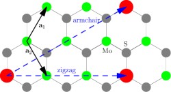
Figure 1: (Color online) Magnetic impurities (red circles) hybridized to Mo $d$-orbitals. Blue dashed arrows show two high-symmetry directions, zigzag and armchair, along which we compare the effective interaction between local moments. Black solid arrows indicate unit vectors.

The first Brillouin zone for the monolayer crystal is hexagonal Mattheiss (1973) with two nonequivalent $K_{1}$ and $K_{-1}$ valleys, in which most of the low energy physics takes place. Lack of reflection symmetry along the $z-$axis in the unit cell produces a splitting of the metal $d$-orbitals resulting in a direct gap at $K_{1}$ and $K_{-1}$ valleys. The high atomic number of the transition metal produces a sizable spin-orbit coupling which further splits the valence bands into two with opposite spin projection Cheiwchanchamnangij and Lambrecht (2012). These two effects result in a strong spin-valley coupling, while spin remains a good quantum number Xiao et al. (2012).

Several recent ab initio calculations show that the (spin-degenerate) valence band valley at the $\Gamma$ point, also contributes to the low energy physics Cheiwchanchamnangij and Lambrecht (2012); Yun et al. (2012); Shi et al. (2013); Kormányos et al. (2013); Zahid et al. (2013). The $\Gamma$ valley participates in virtual transitions even at low p-doping levels (or gating ranges) common in experiments Laskar et al. (2014); Ye et al. (2012); Zhang et al. (2013); Braga et al. (2012); Sik Hwang et al. (2012); Jo et al. (2014).

The proposed effective low energy Hamiltonian to describe these properties is given by:

$$H_{0}=\sum_{q,\tau}\psi^{\dagger}h_{K_{\tau}}(q)\psi+\sum_{k}\phi^{\dagger}h_{\Gamma}(k)\phi,$$ (1)

where

$$h_{K_{\tau}}(q)=\left(\!\!\begin{array}[]{cccc}\xi&a\tau qe^{-i\tau\theta}&0&0\\ a\tau qe^{i\tau\theta}&\lambda(\tau-1)&0&0\\ 0&0&\xi&a\tau qe^{-i\tau\theta}\\ 0&0&a\tau qe^{i\tau\theta}&-\lambda(\tau+1)\end{array}\!\!\right),$$ (2)

is the matrix near the $K_{\tau}$ valleys, $\tau=\pm 1$ is the valley index; $q=|\bf q|$, is the modulus of the reduced wave vector measured from $K_{\tau}$, and $\theta=\arctan(q_{y}/q_{x})$. The spinor bases are arranged as $\psi=(z^{2}\!\uparrow,xy\!\uparrow,z^{2}\!\downarrow,xy\!\downarrow)^{T}$, where $z^{2}$ ($xy$) stands for $\Ket{d_{3z^{2}-r^{2}}}$ ($\left[\Ket{d_{x^{2}-y^{2}}}+i\tau\Ket{d_{xy}}\right]/\sqrt{2}$) Mo $3d$ orbitals, and $\phi=(p_{xy}\!\uparrow,d_{z^{2}}\!\uparrow,p_{xy}\!\downarrow,d_{z^{2}}\!\downarrow)^{T}$, where $p_{xy}$ are S $p_{x},p_{y}$ orbitals. The up/down arrows indicate the $z$-spin projection. Energies are expressed throughout in units of the nearest-neighbor hopping amplitude $t$, $a$ is the nearest Mo-Mo distance, $\xi=\Delta-\lambda$, where $\lambda$ is the spin-orbit coupling constant, and $\Delta$ stands for the gap. Typical values for MoS₂ are $a\simeq 3.2\text{ \AA}$, $t\simeq 1.1\text{ eV}$, so that $\Delta\simeq 1.5$, and $\lambda\simeq 0.07$. The energies have been shifted such that the top of the valence bands at the $K_{\tau}$ points lie at zero energy. At the $\Gamma$ point we have Kormányos et al. (2013)

$$h_{\Gamma}(k)=E_{\Gamma}(k)\left(\!\!\begin{array}[]{cccc}0&0&0&0\\ 0&1&0&0\\ 0&0&0&0\\ 0&0&0&1\end{array}\!\!\right),$$ (3)

where $k$ is the modulus of the wave vector measured from the $\Gamma$ point, $E_{\Gamma}(k)=\hbar^{2}k^{2}/(2tm_{\text{eff}})+\epsilon_{\Gamma}$. $m_{\text{eff}}$ is the (negative) effective mass, and $\epsilon_{\Gamma}$ sets the relative position of the $\Gamma$ and $K_{\tau}$ valleys ($\epsilon_{\Gamma}\approx 0.1$ in MoS₂). The conduction matrix elements were discarded due to the large gap between conduction and valence bands. A schematic representation of the valence band structure around the three relevant points in the Brillouin zone is shown in Fig. 2(d).

Next, we consider two spin-$1/2$ s-wave magnetic impurities hybridized to Mo atoms, given that relevant Bloch states at low energies are composed mainly from admixtures of $d$ orbitals from these atoms. We choose two high symmetry directions connecting these local moments, zigzag and armchair, to show characteristic results, although many other directions are clearly possible— see Fig. 1. The interaction between each magnetic atom and conduction electron spins in the host is described by a contact interaction $H_{\text{int}}=J\sum_{j=1,2}\mathbf{S}_{j}\cdot\mathbf{s}(\mathbf{R}_{j})$, where $\mathbf{s}(\mathbf{r})=\frac{1}{2}\sum_{i}\delta(\mathbf{r}-\mathbf{r}_{i})\boldsymbol{\sigma}_{i}$ represents the spin density for electron $i$ ($\hbar=1$), and $\mathbf{S}_{j}$ is the localized spin at site $\mathbf{R}_{j}$. For simplicity, we assume the same exchange coupling $J$ for valence electrons on both $d_{xy}$ and $d_{z^{2}}$ Mo orbitals. One can treat $H_{\text{int}}$ as a perturbation of $H_{0}$; obtaining at second order an effective interaction between the localized spins Mattis (2006)

$$H_{\text{RKKY}}=J^{2}\sum_{\alpha,\beta}S_{1}^{\alpha}\,\chi_{\alpha,\beta}(\mathbf{R})\,S_{2}^{\beta},$$ (4)

where $\chi_{\alpha,\beta}$ is the static spin susceptibility tensor of the electron gas, with $\alpha,\beta$ representing the Cartesian components, and $\mathbf{R}$ is the vector connecting the magnetic moments. The susceptibility can be calculated from the unperturbed real space retarded Green’s function Imamura et al. (2004); Parhizgar et al. (2013)

$$\begin{split}&\chi_{\alpha,\beta}(\mathbf{R})=\\ &-\frac{1}{\pi}\operatorname{Tr}\left[\int_{-\infty}^{\epsilon_{F}}\!\!d\epsilon\>\operatorname{Im}\left\{\sigma_{\alpha}G(\mathbf{R},\epsilon^{+})\sigma_{\beta}G(-\mathbf{R},\epsilon^{+})\right\}\right],\end{split}$$ (5)

where $\epsilon^{+}=\epsilon+i0^{+}$, and $\sigma$ are Pauli matrices for the spin degree of freedom. $G$ stands for the $2\times 2$ Green’s function matrix for the valence sector—processes that involve the conduction band are ignored, as they are strongly suppressed by the substantial energy gap. Different components of the susceptibility are $\chi_{\alpha,\beta}(\mathbf{R})=-\frac{1}{\pi}\int_{-\infty}^{\epsilon_{F}}\!\!d\epsilon\>\operatorname{Im}A_{\alpha,\beta}(\mathbf{R},\epsilon^{+}),$ with

$$A_{z,z} =\sum_{s}G_{s}(\mathbf{R},\epsilon^{+})G_{s}(-\mathbf{R},\epsilon^{+}),$$ (6)

$$A_{x,x} =A_{y,y}=\sum_{s}G_{s}(\mathbf{R},\epsilon^{+})G_{-s}(-\mathbf{R},\epsilon^{+}),$$ (7)

$$A_{x,y} =-A_{y,x}=-i\sum_{s}s\>G_{s}(\mathbf{R},\epsilon^{+})G_{-s}(-\mathbf{R},\epsilon^{+}),$$ (8)

where $G_{s}(\mathbf{R},\epsilon^{+})=G_{\Gamma}(\mathbf{R},\epsilon^{+})+\sum_{\tau}G_{\tau,s}(\mathbf{R},\epsilon^{+})$, and $s=\uparrow,\downarrow$. The effective anisotropic spin interaction between localized moments includes Ising (ZZ), XX and Dzyaloshinskii-Moriya (DM) interactions, such that the RKKY Hamiltonian can be expressed as Parhizgar et al. (2013)

$$\begin{split}H_{RKKY}=&J_{XX}(S_{1}^{x}S_{2}^{x}+S_{1}^{y}S_{2}^{y})+J_{ZZ}S_{1}^{z}S_{2}^{z}\\ &+J_{DM}(\mathbf{S}_{1}\times\mathbf{S}_{2})_{z},\end{split}$$ (9)

where $J_{XX}=J^{2}\chi_{x,x}$, $J_{ZZ}=J^{2}\chi_{z,z}$, and $J_{DM}=J^{2}\chi_{x,y}$. Notice that the XX and DM terms compete as to favor (anti)parallel or perpendicular alignment of the spins respectively in the $xy$ plane at different impurity separations $\mathbf{R}$, creating in general an in-plane twisted spin structure, depending on their relative strength and sign.

It is convenient to obtain the Green’s functions in momentum space and then Fourier-transform back to real space. sup There are only two independent Green’s functions at $K_{1}$ and $K_{-1}$, $g_{-1,-s}(\mathbf{R},\epsilon^{+})=g_{1,s}(\mathbf{R},\epsilon^{+})$. Omitting the energy variable for convenience, one obtains $G_{s}(\mathbf{R})=G_{\Gamma}(R)+\sum_{\tau}e^{i\mathbf{K}_{\tau}\cdot\mathbf{R}}g_{\tau,s}(R)$, and using Eq. (6), we arrive at

$$\begin{split}\operatorname{Im}\>&A_{z,z}=2\Bigl{(}I_{G_{\Gamma};G_{\Gamma}}+\left[\cos(\mathbf{K}_{1}\cdot\mathbf{R})+\cos(\mathbf{K}_{-1}\cdot\mathbf{R})\right]\\ &\times\left(I_{G_{\Gamma};g_{1,\uparrow}}+I_{G_{\Gamma};g_{-1,\uparrow}}\right)+I_{g_{1,\uparrow};g_{1,\uparrow}}+I_{g_{-1,\uparrow};g_{-1,\uparrow}}\\ &+2\cos\left[(\mathbf{K}_{1}-\mathbf{K}_{-1})\cdot\mathbf{R}\right]I_{g_{1,\uparrow};g_{-1,\uparrow}}\Bigr{)},\end{split}$$ (10)

where we have defined $I_{u;v}(\mathbf{R},\epsilon)\equiv\operatorname{Im}[u(\mathbf{R},\epsilon)v(\mathbf{R},\epsilon)]$ with $u,v=\{G_{\Gamma};g_{1,\uparrow};g_{-1,\uparrow}\}$. A similar procedure yields the $A_{x,x}$ and $A_{x,y}$ components. The cosines are angular coefficients that modulate the integral kernels $I_{u;v}$, depending on the relative direction of the impurities. An interesting feature of these expressions is that the underlying axial symmetries eliminate the DM (or XY) components for impurities arranged along armchair directions sup .

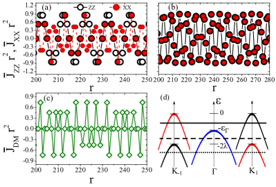
Figure 2: (Color online) ZZ and XX components of the RKKY interaction as function of impurity separation $r$, along (a) zigzag and (b) armchair directions. (c) DM component in the zigzag direction. The latter vanishes in the armchair direction. In all cases the interaction amplitude decays as $r^{-2}$. The Fermi level $\epsilon_{F}\simeq-0.067$, crosses the uppermost $K_{\tau}$ valleys, without intersecting the valley at the $\Gamma$ point, as indicated by the solid line in (d). (d) Schematic low energy band structure for MoS₂ and WS₂, showing the spin inversion of the valence bands at $K_{1}$ and $K_{-1}$ valleys. The black (red) curve corresponds to up (down) spin projection. The blue valley at $\Gamma$ is quadratic and spin degenerate. Dashed and dotted lines indicate higher p-doping levels discussed in Fig. 3 and below.

Fixed Fermi level.—We define the dimensionless exchange interactions as $\bar{J}_{i}=-\frac{\Omega^{2}}{4\pi^{3}J^{2}}J_{i}$, where $i=(ZZ,XX,DM)$, and $\Omega$ is the area of the first Brillouin zone. Let us first analyze the case in which the Fermi level does not intersect the $\Gamma$ valley, i.e. with $-\epsilon_{\Gamma}<\epsilon_{F}<0$, as indicated by the solid horizontal line in Fig. 2(d). $I_{g{1,\uparrow},g{1,\uparrow}}$ is the only kernel contributing to the interaction. Figures 2(a) and (b) show the ZZ and XX components of the RKKY interaction vs impurity separation along the zigzag and armchair directions respectively. The Fermi level is fixed at $\epsilon_{F}\simeq-0.067$, and $\bar{J}_{i}r^{2}$ is plotted as a function of the dimensionless distance $r$ ($=R/a$), for large separations. The nearly constant amplitude reflects that the interaction decays as $1/r^{2}$. In the zigzag case, the XX angular coefficients are related by the sequence $\{1,-1/2,-1/2,\cdots\}$ with the ZZ ones (which are constant) sup , so that the ZZ component tend to dominate over the XX. In the armchair direction, both ZZ and XX components coincide. Moreover, on sites in which $\int_{-\infty}^{\epsilon_{F}}d\epsilon\>I_{g_{1,\uparrow};g_{1,\uparrow}}(r,\epsilon)$ vanishes, both the ZZ and XX components vanish. Figure 2(c) shows the DM component in the zigzag direction, with a sequence $\{0,1,-1.\cdots\}$ with respect to ZZ. As mentioned, the symmetry of the lattice forces this component to vanish along the armchair direction.

In order to examine the spatial oscillations, it is convenient to define $q^{F}_{\pm 1}\equiv q_{\pm}(\epsilon_{F})$ as the Fermi wave vector for the valleys with quantum numbers $\tau=\pm 1,s=\uparrow$, and $\tau=\mp 1,s=\downarrow$, and $k_{\Gamma}^{F}\equiv k_{\Gamma}(\epsilon_{F})$, the Fermi wave vector for the $\Gamma$ valley. With $\epsilon_{F}=-0.067$, the modulation wavelength is $\Lambda\simeq 10$ in the zigzag direction, as observed in Fig. 2(a) and (c), and consistent with $\Lambda=\pi/q_{1}^{F}$. The modulation can be described by a sinusoidal function $\int_{-\infty}^{\epsilon_{F}}d\epsilon\>I_{g_{1,\uparrow};g_{1,\uparrow}}(r,\epsilon)\simeq c_{1}r^{-2}\sin[2q_{1}^{F}r]=c_{1}r^{-2}\sin[2\pi r/\Lambda].$ The amplitude here, $c_{1}\simeq 0.45$, is nearly independent of the Fermi energy. Along the armchair direction the modulation of the interimpurity interaction exhibits a more complex pattern, as observed in Fig. 2(b). Going from the zigzag to armchair directions amounts to replacing $r$ by $\sqrt{3}r$, which can be seen as a shift of $q_{1}^{F}$ to $\sqrt{3}q_{1}^{F}$ in the argument of the integral kernels sup , giving an effective $k_{F}$ that is larger (and incommensurate) than in the zigzag case. The incommensurate value also introduces aliasing effects.

Fig. 3 shows results at $\epsilon_{F}\simeq-0.174$, such that the Fermi level intersects the band at the $\Gamma$ point [dashed line in Fig. 2(d)], for impurities aligned along the zigzag direction.

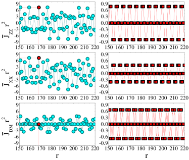
Figure 3: (Color online) ZZ, XX, and DM components of the RKKY interaction, as a function of separation in the zigzag direction. $\epsilon_{F}=-0.174$, as indicated by dashed line in Fig. 2(d). Left panels show the full interactions, including contributions of the $\Gamma$ valley. The red horizontal and vertical lines indicate a fully isotropic interaction point. Right panels show the same quantities without including the $\Gamma$ valley. Notice the different vertical scales.

The right panels show the $r$ dependence of the different interaction components, without the contribution of the $\Gamma$ valley, while the left panels show the full interaction. The inclusion of the $\Gamma$ valley not only increases significantly ($\times 10$) the amplitude of the modulation for all the interactions, but also produces a rather complex oscillatory pattern, due to the additional electron scattering processes between states at $\Gamma$ and $K_{\tau}$ points. The integral kernels contributing significantly in this regime are $I_{G_{\Gamma};G_{\Gamma}}$, $I_{G_{\Gamma};g_{1,\uparrow}}$, and $I_{g_{1,\uparrow};g_{1,\uparrow}}$ sup . A sinusoidal fit gives $\int_{-\infty}^{\epsilon_{F}}d\epsilon\>I_{G_{\Gamma};g_{1,\uparrow}}\simeq c_{2}r^{-2}\sin\left(\left[q_{1}^{F}+k^{F}_{\Gamma}\right]r\right)$, with a wavelength given by $\Lambda=2\pi/[q_{1}^{F}+k_{\Gamma}^{F}]\simeq 4.92$, and $c_{2}\simeq 0.24$; $c_{2}$ is found to be strongly dependent on the Fermi energy. In the limit $\epsilon_{F}\rightarrow-\epsilon_{\Gamma}$, the $\Gamma$ to $K_{\tau}$ scattering processes produce an unusual spatial decay $r^{-5/2}$. However, the weight of this component is small compared to the ones in which the electronic processes take place within the same band valley, so that the expected $r^{-2}$ decay dominates. Notice that the inclusion of the scattering processes at $\Gamma$ allows for special impurity separations in which the DM term vanishes, and $J_{XX}=J_{ZZ}=J_{YY}$, rendering a fully isotropic exchange interaction between them (see for example $r=168$ in the figure). This feature is a consequence of the spin degeneracy at this valley that effectively cancels the DM component. Similar features are observed for impurities separated along the armchair direction.

At higher p-doping, $\epsilon_{F}<-2\lambda$ [dotted line in Fig. 2(d)], all valleys contribute to the indirect exchange, and the interaction exhibits very complex modulation patterns. The oscillations are dominated by $\int_{-\infty}^{\epsilon_{F}}d\epsilon\>I_{\Gamma;g_{-1,\uparrow}}(r,\epsilon)\simeq c_{3}r^{-2}\sin\left(\left[q_{-1}^{F}+k^{F}_{\Gamma}\right]r\right)$, $\int_{-\infty}^{\epsilon_{F}}d\epsilon\>I_{g_{1,\uparrow};g_{-1,\uparrow}}(r,\epsilon)\simeq c_{4}r^{-2}\sin\left(\left[q_{1}^{F}+q_{-1}^{F}\right]r\right)$, and $\int_{-\infty}^{\epsilon_{F}}d\epsilon\>I_{g_{-1,\uparrow};g_{-1,\uparrow}}(r,\epsilon)\simeq c_{5}r^{-2}\sin\left[2q_{-1}^{F}r\right]$, where $c_{3}$ and $c_{4}$ depend strongly on $\epsilon_{F}$, while $c_{5}$ is nearly independent of $\epsilon_{F}$.

Fixed distance.— We now analyze the case where the two impurities remain at a fixed distance along the zigzag direction, and analyze the RKKY interaction over a large Fermi energy range. We set $r=50$ in the data shown below. For $-\epsilon_{\Gamma}<\epsilon_{F}<0$ the $\Gamma$ valley does not contribute to scattering [Fig. 4(a)]; all three components have similar amplitudes, with XX and DM oscillating in phase with each other, but out of phase with ZZ. This indicates an alternation between FM (AFM) in plane order and AFM (FM) out-of-plane order as the energy is shifted.

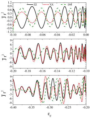
Figure 4: (Color online) Comparison of the different components of the RKKY interaction for different Fermi energy regimes: (a) $-\epsilon_{\Gamma}<\epsilon_{F}<0$, (b) $-2\lambda<\epsilon_{F}<-\epsilon_{\Gamma}$, and (c) $\epsilon_{F}<-2\lambda$. The interimpurity distance is fixed along the zigzag direction at $r=50$. Notice different vertical scales.

When the Fermi energy is positioned in the region $-2\lambda<\epsilon_{F}<-\epsilon_{\Gamma}$, Fig. 4(b), the ZZ and XX interactions become in phase, while the DM modulation retains a longer period. This is caused by the absence of the term $I_{G_{\Gamma};G_{\Gamma}}$, because the $\Gamma$ valley is unaffected by the spin-orbit interaction. In this case an isotropic exchange exists at particular values of $\epsilon_{F}$ for a vanishing DM component. At deeper Fermi energy, $\epsilon_{F}<-2\lambda$, with all valleys contributing, one finds very interesting behavior: For $\epsilon_{F}\lesssim-0.35$, there exists another isotropic interaction regime with the ZZ and XX components contributing equally and the DM term weaker or even zero.

Conclusions.— We have shown that inclusion of the $\Gamma$ valley, neglected in previous studies, changes predicted magnetic order for RKKY interacting impurities deposited on TMD materials. By judicious choice of impurity separation, level doping or gating, it is possible to alternate between isotropic and anisotropic order as well as to have well defined (or not) in-plane order by manipulating the strength of the DM interaction. The results described above show behavior that can be readily tested by experiments, such as spin polarized STM Zhou et al. (2010); Khajetoorians et al. (2012). Note that although we have focused on MoS₂, our results are applicable to other dichalcogenides, specially WS₂ that appears to be easier to dope (or gate). Characterization of the interaction between magnetic impurities with doping level would also provide an interesting but direct approach to determine the splitting of the $\Gamma$ valley in real systems.

Acknowledgments.— This work was supported in part by NSF MWN/CIAM grant DMR-1108285.

Supplemental Material

Detailed calculation of the RKKY interaction

We start with the Green’s functions in momentum space. For the $K_{\tau}$ valleys, one gets Parhizgar et al. (2013)

$$G_{\tau,s}(q,\epsilon^{+})=(\epsilon^{+}-\xi)[(\epsilon^{+}-\xi)(\epsilon^{+}+\lambda[1-\tau s])-a^{2}q^{2}]^{-1},$$ (11)

while at the $\Gamma$ point we have

$$G_{\Gamma}(k,\epsilon^{+})=[\epsilon^{+}-E_{\Gamma}(k)]^{-1}.$$ (12)

We then apply Fourier transforms as

$$G_{\Gamma}(\mathbf{R},\epsilon^{+})=\frac{1}{\hat{\Omega}}\int d\mathbf{k}\,\,e^{i\mathbf{k}\cdot\mathbf{R}}G_{\Gamma}(k,\epsilon^{+}),$$ (13)

and

$$G_{\tau,s}(\mathbf{R},\epsilon^{+})=\frac{1}{\hat{\Omega}}\int d\mathbf{k}\,\,e^{i\mathbf{k}\cdot\mathbf{R}}G_{\tau,s}(q,\epsilon^{+})=e^{i\mathbf{K}_{\tau}\cdot\mathbf{R}}g_{\tau,s}(\mathbf{R},\epsilon^{+}),$$ (14)

where

$$g_{\tau,s}(\mathbf{R},\epsilon^{+})=\frac{1}{\hat{\Omega}}\int d\mathbf{q}\,\,e^{i\mathbf{q}\cdot\mathbf{R}}G_{\tau,s}(q,\epsilon^{+}),$$ (15)

and $\hat{\Omega}$ is the area of the first Brillouin zone. Notice that the factor $e^{i\mathbf{K}_{\tau}\cdot\mathbf{R}}$ in Eq. (14) appears because the original Green’s functions for valleys $K_{\tau}$ are expressed in terms of the reduced wave vector $\mathbf{q}$, while the Fourier transform integrates in the momentum $\mathbf{k}$ measured from the $\Gamma$ point. From the expressions above, it is easy to observe that $g_{\tau,s}(-\mathbf{R},\epsilon^{+})=g_{\tau,s}(\mathbf{R},\epsilon^{+})$, $G_{\Gamma}(-\mathbf{R},\epsilon^{+})=G_{\Gamma}(\mathbf{R},\epsilon^{+})$, and $G_{\tau,s}(-\mathbf{R},\epsilon^{+})=e^{-i\mathbf{K}_{\tau}\cdot\mathbf{R}}g_{\tau,s}(\mathbf{R},\epsilon^{+})$.

The Fourier transforms involve exponential factors of the form $e^{i\mathbf{k}\cdot\mathbf{R}}=e^{ikR\cos(\theta_{R}-\theta_{k})}$, where $\theta_{R}$ ($\theta_{k}$) is the angle of the interimpurity distance vector (wave vector) measured from the positive $x$ axis. Using the Jacobi-Anger expansion Gradshteyn and Ryzhik (1980)

$$e^{ikR\cos(\theta_{R}-\theta_{k})}=J_{0}(kR)+2\sum_{n=1}^{\infty}i^{n}J_{n}(kR)\cos[n(\theta_{R}-\theta_{k})],$$ (16)

where $J_{n}$ are Bessel functions of the first kind and order $n$, we can write

$$G_{\Gamma}(R,\epsilon^{+})=\frac{1}{\hat{\Omega}}\int\!d\mathbf{k}\frac{e^{i\mathbf{k}\cdot\mathbf{R}}}{\epsilon^{+}-E_{\Gamma}(k)}=\frac{2\pi}{\hat{\Omega}}\int_{0}^{\infty}\!\!dk\frac{kJ_{0}(kR)}{\epsilon^{+}-E_{\Gamma}(k)}=-\frac{4\pi m_{\text{eff}}t}{\hat{\Omega}\hbar^{2}}\int_{0}^{\infty}dk\frac{kJ_{0}(kR)}{k^{2}+\left[i\sqrt{\frac{2m_{\text{eff}}t}{\hbar^{2}}(\epsilon^{+}+\epsilon_{\Gamma})}\right]^{2}}.$$ (17)

Notice that, after the integration over the angle $\theta_{k}$, the remaining integral over the magnitude of the momentum is evaluated from $0$ to $\infty$. To be completely accurate, one should introduce a high momentum cutoff. However, as one is usually interested in the large distance behavior of the interaction, it it expected that the momenta above this cutoff have a negligible contribution to the integral, so the integration up to $k\rightarrow\infty$ is exact for practical purposes. Using the fact that

$$\int_{0}^{\infty}dk\frac{kJ_{0}(kR)}{k^{2}+\alpha^{2}}=K_{0}[\alpha\operatorname{sgn}(\operatorname{Re}\alpha)R],$$ (18)

where $K_{0}$ is an order zero modified Bessel function of the second kind, and sgn is the sign function, one can rewrite Eq. (17) as

$$G_{\Gamma}(R,\epsilon^{+}) =-\frac{4\pi m_{\text{eff}}t}{\hat{\Omega}\hbar^{2}}K_{0}\bigg{[}-i\sqrt{\frac{2m_{\text{eff}}t}{\hbar^{2}}(\epsilon^{+}+\epsilon_{\Gamma})}R\bigg{]}.$$ (19)

At this point it is convenient to define dimensionless parameters: $r\equiv R/a$, where $a$ is the closest Mo-Mo distance, $\Omega\equiv\hat{\Omega}a^{2}$, $\gamma\equiv-2m_{\text{eff}}ta^{2}/\hbar^{2}$. For MoS₂, $m_{\text{eff}}\simeq-2.6\ m_{\text{el}}$ Jin et al. (2013); Kormányos , so we get $\gamma\simeq 7.67$. Using these conventions, we get the dimensionless Green’s function,

$$G_{\Gamma}(r,\epsilon^{+}) =\frac{2\pi\gamma}{\Omega}K_{0}\bigl{[}\sqrt{\gamma(\epsilon^{+}+\epsilon_{\Gamma})}r\bigr{]}.$$ (20)

Now we can expand the argument of the Bessel function as

$$\sqrt{\gamma(\epsilon^{+}+\epsilon_{\Gamma})}=\begin{cases}\sqrt{\gamma(\epsilon+\epsilon_{\Gamma})}+i\frac{\eta}{2}\sqrt{\frac{\gamma}{\epsilon+\epsilon_{\Gamma}}}&\epsilon>-\epsilon_{\Gamma},\\ \frac{\eta}{2}\sqrt{-\frac{\gamma}{\epsilon+\epsilon_{\Gamma}}}+i\sqrt{-\gamma(\epsilon+\epsilon_{\Gamma})}&\epsilon<-\epsilon_{\Gamma},\end{cases}$$ (21)

such that, for $\eta\rightarrow 0^{+}$, one gets

$$\begin{split}G_{\Gamma}(r,\epsilon^{+})&=\frac{2\pi\gamma}{\Omega}\Bigl{(}K_{0}\bigl{[}\sqrt{\gamma(\epsilon+\epsilon_{\Gamma})}r\bigr{]}\theta(\epsilon+\epsilon_{\Gamma})+K_{0}\bigl{[}i\sqrt{-\gamma(\epsilon+\epsilon_{\Gamma})}r\bigr{]}\bigl{[}1-\theta(\epsilon+\epsilon_{\Gamma})\bigr{]}\Bigr{)},\end{split}$$ (22)

where $\theta$ stands for the Heaviside step function. From this expression, one can see that the Green’s function comprises two parts. The first one, when $\epsilon>-\epsilon_{\Gamma}$, is decaying and accounts for virtual processes in which an electron tunnels out of the band. The second one, for $\epsilon<-\epsilon_{\Gamma}$, is oscillating. We can rewrite this expression by using the identities Gradshteyn and Ryzhik (1980)

$$K_{\nu}(z) =-\frac{i\pi}{2}e^{-i\pi\nu/2}H_{\nu}^{(2)}(-iz),$$ (23)

$$H_{\nu}^{(2)}(z) =J_{\nu}(z)-iY_{\nu}(z),$$ (24)

where $Y_{\nu}(z)$ are Bessel functions of the second kind, and $H_{\nu}^{(2)}(z)$ are Hankel functions. We arrive to

$$G_{\Gamma}(r,\epsilon^{+})=\frac{\pi^{2}\gamma}{\Omega}\Bigl{[}\frac{2}{\pi}K_{0}\left[\sqrt{\gamma(\epsilon+\epsilon_{\Gamma})}r\right]\theta(\epsilon+\epsilon_{\Gamma})-\left(iJ_{0}\big{[}\sqrt{-\gamma(\epsilon+\epsilon_{\Gamma})}r\big{]}+Y_{0}\left[\sqrt{-\gamma(\epsilon+\epsilon_{\Gamma})}r\right]\right)\left(1-\theta(\epsilon+\epsilon_{\Gamma})\right)\Bigr{]}.$$ (25)

The same procedure can be applied at the $K_{\tau}$ points

$$\begin{split}g_{\tau,s}(r,\epsilon^{+})&=-\frac{2\pi}{\Omega}(\epsilon^{+}-\xi)\int_{0}^{\infty}\!\!dq\frac{qJ_{0}(qr)}{q^{2}+\Bigl{(}\frac{i}{a}\sqrt{(\epsilon^{+}-\xi)(\epsilon^{+}+\lambda[1-\tau s])}\Bigr{)}^{2}},\end{split}$$ (26)

or

$$g_{\tau,s}(r,\epsilon^{+})=-\frac{2\pi}{\Omega}K_{0}\Bigl{[}i\sqrt{(\epsilon^{+}-\xi)(\epsilon^{+}+\lambda[1-\tau s])}\operatorname{sgn}\operatorname{Re}\big{\{}i\sqrt{(\epsilon^{+}-\xi)(\epsilon^{+}+\lambda[1-\tau s])}\big{\}}r\Bigr{]}.$$ (27)

To get more insight into this expression, let us define $\mathcal{Z}=(\tilde{\epsilon}^{+}-\Delta+\lambda)(\tilde{\epsilon}^{+}+\lambda[1-\tau s])$, so $\operatorname{Re}\mathcal{Z}=\tilde{\epsilon}^{2}-\eta^{2}+\tilde{\epsilon}(\lambda[2-\tau s]-\Delta)+\lambda(\lambda-\Delta)(1-\tau s)$, and $\operatorname{Im}\mathcal{Z}=\eta(2\tilde{\epsilon}+\lambda(2-\tau s)-\Delta)$. We have that, for $\eta\rightarrow 0$, $\operatorname{Re}\mathcal{Z}=0$ when $\tilde{\epsilon}^{2}+\tilde{\epsilon}(\lambda[2-\tau s]-\Delta)+\lambda(\lambda-\Delta)(1-\tau s)=0$, whose solutions are

$$\begin{split}\tilde{\epsilon}_{\tau,s}^{\pm}&=\frac{1}{2}\bigg{[}\Delta-\lambda(2-\tau s)\pm\sqrt{[\Delta-\lambda(2-\tau s)]^{2}-4\lambda(\lambda-\Delta)(1-\tau s)}\bigg{]}.\end{split}$$ (28)

For the cases in which $\tau s=1$, we have $\tilde{\epsilon}_{1,\uparrow}^{\pm}=\tilde{\epsilon}_{-\!1,\downarrow}^{\pm}\equiv\tilde{\epsilon}_{1}^{\pm}=\frac{1}{2}\big{[}\Delta-\lambda\pm|\Delta-\lambda|\big{]}$. Moreover, $(\operatorname{Re}\mathcal{Z})^{\prime}=2>0$, so we have a parabola with positive concavity crossing the $\tilde{\epsilon}$-axis at 0 and at $\Delta-\lambda>0$. If we consider that the Fermi energy is always in the valence bands, $\epsilon_{F}<0$, then $\operatorname{Re}\mathcal{Z}>0,\forall\epsilon$ if $\tau s=1$.

For the case in which $\tau s=-1$, we have $\tilde{\epsilon}_{-\!1,\uparrow}^{\pm}=\tilde{\epsilon}_{1,\downarrow}^{\pm}\equiv\tilde{\epsilon}_{-\!1}^{\pm}=\frac{1}{2}\Bigl{[}\Delta-3\lambda\pm(\Delta+\lambda)\Bigr{]}$, or

$$\begin{cases}\tilde{\epsilon}_{-\!1}^{+}&=(\Delta-\lambda)>0,\\ \tilde{\epsilon}_{-\!1}^{-}&=-2\lambda<0.\end{cases}$$ (29)

Then $\operatorname{Re}\mathcal{Z}>0$ if $\epsilon<\tilde{\epsilon}_{-\!1}^{-}$ and $\operatorname{Re}\mathcal{Z}<0$ if $\tilde{\epsilon}_{-\!1}^{-}<\epsilon<0$. Finally, $\operatorname{Im}\mathcal{Z}<0\,\,\forall\,\,\tau s$. The two independent Green’s function are

$$\begin{split}g_{1,\uparrow}(r,\epsilon^{+})&=-\frac{2\pi}{\Omega}(\epsilon^{+}-\xi)K_{0}\left[i\sqrt{\epsilon(\epsilon-\xi)}r\right]=\frac{\pi^{2}}{\Omega}(\epsilon^{+}-\xi)\Bigl{(}iJ_{0}\left[\sqrt{\epsilon(\epsilon-\xi)}r\right]+Y_{0}\left[\sqrt{\epsilon(\epsilon-\xi)}r\right]\Bigr{)},\\ g_{-\!1,\uparrow}(r,\epsilon^{+})&=-\frac{2\pi}{\Omega}(\epsilon^{+}-\xi)\Bigl{\{}K_{0}\left[i\sqrt{(\epsilon+2\lambda)(\epsilon-\xi)}r\right]\left[1-\Theta(\epsilon+2\lambda)\right]+K_{0}\left[\sqrt{-(\epsilon+2\lambda)(\epsilon-\xi)}r\right]\Theta(\epsilon+2\lambda)\Bigr{\}}\\ &=\frac{\pi^{2}}{\Omega}(\epsilon^{+}-\Delta+\lambda)\Bigl{\{}\Bigl{(}iJ_{0}\left[\sqrt{(\epsilon+2\lambda)(\epsilon-\xi)}r\right]+Y_{0}\left[\sqrt{(\epsilon+2\lambda)(\epsilon-\xi)}r\right]\Bigr{)}\left[1-\Theta(\epsilon+2\lambda)\right]\\ &-\frac{2}{\pi}K_{0}\left[\sqrt{-(\epsilon+2\lambda)(\epsilon-\xi)}r\right]\Theta(\epsilon+2\lambda)\Bigr{\}}.\end{split}$$ (30)

Now we get the expressions for $\operatorname{Im}A_{\alpha,\beta}(\mathbf{r})$, which can be subdivided into different terms. To simplify the expressions, we define dimensionless wave vectors for the different bands, as a function of the energy

$$k_{\Gamma}(\epsilon) =\sqrt{-\gamma(\epsilon+\epsilon_{\Gamma})},$$

$$q_{1}(\epsilon) =\sqrt{\epsilon(\epsilon-\xi)},$$ (31)

$$q_{-1}(\epsilon) =\sqrt{(\epsilon+2\lambda)(\epsilon-\xi)}.$$

We have different components in $A_{\alpha,\beta}(\mathbf{r})$, whose in-plane contributions to the susceptibility are given by

$$\begin{split}\operatorname{Im}\>A_{z,z}(\mathbf{R})&=2\Bigl{(}I_{G_{\Gamma};G_{\Gamma}}+\left[\cos(\mathbf{K}_{1}\cdot\mathbf{R})+\cos(\mathbf{K}_{-1}\cdot\mathbf{R})\right]\left(I_{G_{\Gamma};g_{1,\uparrow}}+I_{G_{\Gamma};g_{-1,\uparrow}}\right)\\ &+I_{g_{1,\uparrow};g_{1,\uparrow}}+I_{g_{-1,\uparrow};g_{-1,\uparrow}}+2\cos\left[(\mathbf{K}_{1}-\mathbf{K}_{-1})\cdot\mathbf{R}\right]I_{g_{1,\uparrow};g_{-1,\uparrow}}\Bigr{)},\end{split}$$ (32)

$$\begin{split}\operatorname{Im}\>A_{x,x}(\mathbf{R})&=2\Bigl{(}I_{G_{\Gamma};G_{\Gamma}}+\left[\cos(\mathbf{K}_{1}\cdot\mathbf{R})+\cos(\mathbf{K}_{-1}\cdot\mathbf{R})\right]\left(I_{G_{\Gamma};g_{1,\uparrow}}+I_{G_{\Gamma};g_{-1,\uparrow}}\right)\\ &+\cos\left[(\mathbf{K}_{1}-\mathbf{K}_{-1})\cdot\mathbf{R}\right]\left[I_{g_{1,\uparrow};g_{1,\uparrow}}+I_{g_{-1,\uparrow};g_{-1,\uparrow}}\right]+2I_{g_{1,\uparrow};g_{-1,\uparrow}}\Bigr{)},\end{split}$$ (33)

and

$$\begin{split}\operatorname{Im}\>A_{x,y}(\mathbf{R})&=2\Bigl{(}\left[\sin(\mathbf{K}_{1}\cdot\mathbf{R})-\sin(\mathbf{K}_{-1}\cdot\mathbf{R})\right]\left(I_{G_{\Gamma};g_{1,\uparrow}}-I_{G_{\Gamma};g_{-1,\uparrow}}\right)\\ &+\sin\left[(\mathbf{K}_{1}-\mathbf{K}_{-1})\cdot\mathbf{R}\right]\left[I_{g_{1,\uparrow};g_{1,\uparrow}}-I_{g_{-1,\uparrow};g_{-1,\uparrow}}\right]\Bigr{)},\end{split}$$ (34)

with

$$\begin{split}I_{G_{\Gamma};G_{\Gamma}}&(r,\epsilon)=\frac{2\pi^{4}\gamma^{2}}{\Omega^{2}}J_{0}\left[k_{\Gamma}(\epsilon)r\right]Y_{0}\left[k_{\Gamma}(\epsilon)r\right]\left[1-\Theta(\epsilon+\epsilon_{\Gamma})\right],\end{split}$$ (35)

$$\begin{split}I_{G_{\Gamma};g_{1,\uparrow}}(r,\epsilon)&=\frac{\pi^{4}\gamma}{\Omega^{2}}(\epsilon-\xi)\Bigl{\{}\frac{2}{\pi}J_{0}\left[q_{1}(\epsilon)r\right]K_{0}\left[-ik_{\Gamma}(\epsilon)r\right]\Theta(\epsilon+\epsilon_{\Gamma})\\ &-\Bigl{(}J_{0}\left[q_{1}(\epsilon)r\right]Y_{0}\left[k_{\Gamma}(\epsilon)r\right]+Y_{0}\left[q_{1}(\epsilon)r\right]J_{0}\left[k_{\Gamma}(\epsilon)r\right]\Bigr{)}\left[1-\Theta(\epsilon+\epsilon_{\Gamma})\right]\Bigr{\}},\end{split}$$ (36)

$$\begin{split}I_{G_{\Gamma};g_{-1,\uparrow}}(r,\epsilon)&=\frac{\pi^{4}\gamma}{\Omega^{2}}(\epsilon-\xi)\Bigl{\{}\frac{2}{\pi}J_{0}\left[k_{\Gamma}(\epsilon)r\right]K_{0}\left[-iq_{-1}(\epsilon)r\right]\left[1-\Theta(\epsilon+\epsilon_{\Gamma})\right]\Theta(\epsilon+2\lambda)\\ &-\Bigl{(}J_{0}\left[k_{\Gamma}(\epsilon)r\right]Y_{0}\left[q_{-1}(\epsilon)r\right]+Y_{0}\left[k_{\Gamma}(\epsilon)r\right]J_{0}\left[q_{-1}(\epsilon)r\right]\Bigr{)}\left[1-\Theta(\epsilon+2\lambda)\right]\Bigr{\}},\end{split}$$ (37)

$$\begin{split}I_{g_{1,\uparrow};g_{-1,\uparrow}}(r,\epsilon)&=\frac{\pi^{4}}{\Omega^{2}}(\epsilon-\xi)^{2}\Bigl{\{}\Bigl{(}J_{0}\left[q_{1}(\epsilon)r\right]Y_{0}\left[q_{-1}(\epsilon)r\right]+Y_{0}\left[q_{1}(\epsilon)r\right]J_{0}\left[q_{-1}(\epsilon)r\right]\Bigr{)}\\ &\times\left[1-\Theta(\epsilon+2\lambda)\right]-\frac{2}{\pi}J_{0}\left[q_{1}(\epsilon)r\right]K_{0}\left[-iq_{-1}(\epsilon)r\right]\Theta(\epsilon+2\lambda)\Bigr{\}},\end{split}$$ (38)

$$\begin{split}I_{g_{1,\uparrow};g_{1,\uparrow}}(r,\epsilon)&=\frac{2\pi^{4}}{\Omega^{2}}(\epsilon-\xi)^{2}J_{0}\left[q_{1}(\epsilon)r\right]Y_{0}\left[q_{1}(\epsilon)r\right],\end{split}$$ (39)

and

$$\begin{split}I_{g_{-1,\uparrow};g_{-1,\uparrow}}&(r,\epsilon)=\frac{2\pi^{4}}{\Omega^{2}}(\epsilon-\xi)^{2}J_{0}\left[q_{-1}(\epsilon)r\right]Y_{0}\left[q_{-1}(\epsilon)r\right].\end{split}$$ (40)

In order to get the static susceptibility $\chi_{\alpha,\beta}(r)$, we need to integrate these expressions over energy. The one corresponding to Eq. (35) can be integrated analytically, due to its conventional two dimensional parabolic band character Fischer and Klein (1975). Defining $u(\epsilon)=k_{\Gamma}(\epsilon)r$, one gets

$$\int_{-\infty}^{\epsilon_{F}}d\epsilon\,\,I_{G_{\Gamma};G_{\Gamma}}(r,\epsilon)=\frac{4\pi^{4}\gamma}{\Omega^{2}r^{2}}\int_{u(\epsilon_{F})}^{\infty}du\,\,uJ_{0}[u]Y_{0}[u].$$ (41)

This integral can be separated into two terms as $\int_{u(\epsilon_{F})}^{\infty}du=\int_{0}^{\infty}du-\int_{0}^{u(\epsilon_{F})}du$, and using the fact that $\int_{0}^{\infty}du=0$, results in

$$\begin{split}\int_{-\infty}^{\epsilon_{F}}d\epsilon\>I_{G_{\Gamma};G_{\Gamma}}(r,\epsilon)&=-\frac{4\pi^{4}\gamma}{\Omega^{2}r^{2}}\int_{0}^{u(\epsilon_{F})}du\,\,uJ_{0}[u]Y_{0}[u]\\ &=-\frac{2\pi^{4}\gamma[k_{\Gamma}(\epsilon_{F})]^{2}}{\Omega^{2}}\left(J_{0}[k_{\Gamma}(\epsilon_{F})r]Y_{0}[k_{\Gamma}(\epsilon_{F})r]+J_{1}[k_{\Gamma}(\epsilon_{F})r]Y_{1}[k_{\Gamma}(\epsilon_{F})r]\right),\end{split}$$ (42)

For large interimpurity distances, $r\gg 1$, we can approximate the above expression as

$$\int_{-\infty}^{\epsilon_{F}}d\epsilon\,\,I_{G_{\Gamma};G_{\Gamma}}(r,\epsilon)=\frac{2\pi^{3}\gamma}{\Omega^{2}}\frac{\sin\left[2k_{\Gamma}(\epsilon_{F})r\right]}{r^{2}}.$$ (43)

The remaining integrals should be performed numerically and the integration requires some care. They should be regularized by a smooth energy cutoff function, as discussed in Ref. Saremi, 2007. We tried different cutoff functions in order to test convergence. As discussed in the main text, these integrals can be fitted by sinusoidal functions with prefactors that can depend or not of the Fermi energy. Two examples are shown in Fig. 5 for $\epsilon_{F}=-0.174$. The left panel shows the sinusoidal fitting to $r^{2}\int_{-\infty}^{\epsilon_{F}}d\epsilon\,\,I_{G_{\Gamma};g_{1,\uparrow}}(r,\epsilon)\simeq 0.24\sin(1.278\>r)$, and the right panel corresponds to the one for $r^{2}\int_{-\infty}^{\epsilon_{F}}d\epsilon\,\,I_{g_{1,\uparrow};g_{1,\uparrow}}(r,\epsilon)\simeq 0.45\sin(1.047\>r)$.

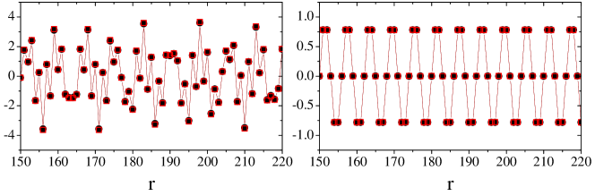
Figure 5: Sinusoidal fittings (red squares) to the energy integrals (black circles) of $I_{G_{\Gamma};g_{1,\uparrow}}$ (left panel) and $I_{g_{1,\uparrow};g_{1,\uparrow}}$ (right panel), as discussed in the text.

Angular dependence of the interaction

The angular dependence enters in different combinations of $\mathbf{K}_{\tau}\cdot\mathbf{R}$ [see Eqs. (32) - (34)]. The vector that connects the impurities can be written as $\mathbf{R}=m\mathbf{a}_{1}+n\mathbf{a}_{2}$, where $\mathbf{a}_{1/2}=\frac{a}{2}(1,\pm\sqrt{3})$, $m,n\in\mathbb{Z}$, and $\mathbf{a}_{i}$ are the primitive vectors (see Fig. 1 in the main text); in dimensionless form, $\mathbf{r}=\mathbf{R}/a=\frac{1}{2}\left(m+n,\sqrt{3}(m-n)\right)$, with $r=\sqrt{(m-n)^{2}+mn}$. We can also define dimensionless valley vectors as $\widetilde{\mathbf{K}}_{\tau}=a\mathbf{K}_{\tau}$, such that $\mathbf{K}_{\tau}\cdot\mathbf{R}=\widetilde{\mathbf{K}}_{\tau}\cdot\mathbf{r}=\pi\left[\left(\frac{\tau}{3}+1\right)m+\left(\frac{\tau}{3}-1\right)n\right]$, and $(\widetilde{\mathbf{K}}_{1}-\widetilde{\mathbf{K}}_{-1})\cdot\mathbf{r}=\frac{2\pi}{3}\left(m+n\right)$. Three zigzag directions are possible, for $(m,n)$ combinations given by $(p,0)$, $(0,p)$ and $(p,p)$, with integer $p$, and $r=|p|$, where the angular coefficients are shown in Table 1.

Zigzag
Coefficient	Direction	Sequence
$\cos[(\widetilde{\mathbf{K}}_{1}-\widetilde{\mathbf{K}}_{-1})\cdot\boldsymbol{r}]$	all	$1$, $-\frac{1}{2}$, $-\frac{1}{2}$,$\cdots$
$\cos[\widetilde{\mathbf{K}}_{1}\cdot\boldsymbol{r}]$	all
$\cos[\widetilde{\mathbf{K}}_{-1}\cdot\boldsymbol{r}]$	all
$\sin[(\widetilde{\mathbf{K}}_{1}-\widetilde{\mathbf{K}}_{-1})\cdot\boldsymbol{r}]$	(p, 0); (0, p)	$0$, $\frac{\sqrt{3}}{2}$, $-\frac{\sqrt{3}}{2}$,$\cdots$
$\sin[\widetilde{\mathbf{K}}_{1}\cdot\boldsymbol{r}]$	(p, p)
$\sin[\widetilde{\mathbf{K}}_{-1}\cdot\boldsymbol{r}]$	(p, 0); (0, p)
$\sin[(\widetilde{\mathbf{K}}_{1}-\widetilde{\mathbf{K}}_{-1})\cdot\boldsymbol{r}]$	(p, p)	$0$, $-\frac{\sqrt{3}}{2}$, $\frac{\sqrt{3}}{2}$,$\cdots$
$\sin[\widetilde{\mathbf{K}}_{1}\cdot\boldsymbol{r}]$	(p, 0); (0, p)
$\sin[\widetilde{\mathbf{K}}_{-1}\cdot\boldsymbol{r}]$	(p, p)

Table 1: Sequences of angular dependent coefficients for the zigzag directions.

The armchair directions are given by $(2p,p)$, $(p,2p)$, $(p,-p)$, so $r=\sqrt{3}|p|$. The coefficients in the armchair direction are simpler than for zigzag, as $\cos(\widetilde{\mathbf{K}}_{\tau}\cdot\boldsymbol{r})=\cos[(\widetilde{\mathbf{K}}_{1}-\widetilde{\mathbf{K}}_{-1})\cdot\boldsymbol{r}]=1$ and $\sin(\widetilde{\mathbf{K}}_{\tau}\cdot\boldsymbol{r})=\sin[(\widetilde{\mathbf{K}}_{1}-\widetilde{\mathbf{K}}_{-1})\cdot\boldsymbol{r}]=0$. This means that in the armchair direction the DM component is always zero due to symmetry.