Opacities and spectra of hydrogen atmospheres of moderately magnetized neutron stars

Abstract

Context. There is observational evidence that central compact objects (CCOs) in supernova remnants have moderately strong magnetic fields $B\sim 10^{11}$ G. Meanwhile, available models of partially ionized hydrogen atmospheres of neutron stars with strong magnetic fields are restricted to $B\gtrsim 10^{12}$ G. Extension of the applicability range of the photosphere models to smaller field strengths is complicated by a stronger asymmetry of decentered atomic states and by the importance of excited bound states.

Aims. We extend the equation of state and radiative opacities, presented in previous papers for $10^{12}\mbox{ G}\lesssim B\lesssim 10^{15}$ G, to weaker fields.

Methods. We construct analytical fitting formulae for binding energies, sizes, and oscillator strengths for different bound states of a hydrogen atom moving in moderately strong magnetic fields and calculate an extensive database for photoionization cross sections of such atoms. Using these atomic data, in the framework of the chemical picture of plasmas we solve the ionization equilibrium problem and calculate thermodynamic functions and basic opacities of partially ionized hydrogen plasmas at these field strengths. Then plasma polarizabilities are calculated from the Kramers-Kronig relation, and the radiative transfer equation for the coupled normal polarization modes is solved to obtain model spectra.

Results. An equation of state and radiative opacities for a partially ionized hydrogen plasma are obtained at magnetic fields $B$, temperatures $T$, and densities $\rho$ typical for atmospheres of CCOs and other isolated neutron stars with moderately strong magnetic fields. The first- and second-order thermodynamic functions, monochromatic radiative opacities, and Rosseland mean opacities are calculated and tabulated, taking account of partial ionization, for $3\times 10^{10}\mbox{ G}\lesssim B\lesssim 10^{12}$ G, $10^{5}$ K $\lesssim T\lesssim 10^{7}$ K, and a wide range of densities. Atmosphere models and spectra are calculated to verify the applicability of the results and to determine the range of magnetic fields and effective temperatures where the incomplete ionization of the hydrogen plasma is important.

1 Introduction

Thermal or thermal-like radiation has been detected from several classes of neutron stars, which are characterized by different typical values of magnetic field $B$. Particularly interesting are isolated neutron stars with clearly observed thermal emission in quiescence, whose thermal X-ray spectra formed at the surface are not blended with emission from accreting matter or magnetosphere (see the list of their properties in Viganò et al. 2013). Most of them have surface magnetic fields in the range $10^{12}\mbox{ G}\lesssim B\lesssim 10^{15}$ G, but one class of sources, so called central compact objects (CCOs) have $B\sim\mbox{a few}\times(10^{10}$ – $10^{11})$ G (Halpern and Gotthelf 2010; Ho 2013). These fields are sufficiently strong to radically affect properties of hydrogen atoms and strongly quantize the electrons in the neutron-star atmosphere, but they are below the field strengths available in the previously developed models of strongly magnetized partially ionized hydrogen atmospheres of neutron stars, which are currently included in the XSPEC package (Arnaud 1996) under the names NSMAX (Ho et al. 2008) and NSMAXG (Ho 2014). Therefore a construction of neutron-star photosphere models for moderately strong magnetic fields has become a topical problem. In this paper we construct such models for $3\times 10^{10}<B<10^{12}$ G.

We use the theoretical model of a partially ionized hydrogen plasma (Potekhin et al. 1999; hereafter Paper I) that was previously used for opacity calculations at $10^{12}\mbox{\leavevmode\nobreak\ G}\lesssim B\lesssim 10^{15}$ G (Potekhin & Chabrier 2003, 2004; hereafter Papers II and III, respectively). However, the present task is more arduous, because the field strength is closer to the atomic unit $B_{0}={m_{\mathrm{e}}^{2}\,c\,e^{3}}/{\hbar^{3}}=2.35\times 10^{9}$ G. Accordingly, the dimensionless magnetic field parameter $\gamma=B/B_{0}$ is smaller, and the adiabatic approximation for atomic wave functions, which is valid at $\gamma\to\infty$, becomes less adequate, which entails the need to include more terms than previously in the wave-function expansion beyond this approximation.

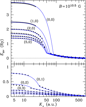
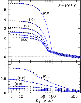
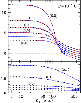
Figure 1: Binding energies of different states ($s,\nu$) of a hydrogen atom as functions of pseudomomentum $K_{\perp}$ at $B=3.16\times 10^{10}$ G (left), $B=10^{11}$ G (middle), and $B=10^{12}$ G (right). Numerical calculations (dots) are compared with the analytical approximation presented in Appendix A.1 (solid lines). For comparison, the fit previously developed for $B\gtrsim 10^{12}$ G (Potekhin 1998) is shown by the dashed lines in the upper right panel.

In addition, with decreasing $B$, the energy spectrum of the bound states of a magnetized atom becomes denser, which necessitates inclusion of more such states in the consideration. Meanwhile, since $\gamma\gg 1$, the center-of mass motion of the atom noticeably affects the atomic properties. In order to cope with the problem, we construct analytical fitting formulae for atomic energies, sizes, and main oscillator strengths as functions of $B$, discrete quantum numbers of initial and final states, and pseudomomentum $K_{\perp}$, which corresponds to the state of motion of an atom across the field. These analytical expressions are valid for $\gamma\sim 10$ – 1000 and supplement the previously available fits for larger $\gamma$ (Potekhin 1998). For bound-free transitions, we calculate extensive tables of cross sections as functions of $K_{\perp}$ and photon frequency $\omega$ for a number of bound states at every given $B$ and interpolate across these tables to calculate the opacities in the same way as in Papers II and III.

In Sect. 2 we recall the main properties that characterize the motion of a hydrogen atom in a magnetic field. In Sect. 3 we describe the solution of the ionization equilibrium problem. Section 4 contains the summary of the theoretical methods used to calculate the opacities and polarization vectors of normal electromagnetic modes in a magnetized plasma. Results of numerical calculations are presented and discussed in Sect. 5. In Sect: 6 we formulate conclusions. In the Appendix we present analytical approximations to the results of numerical calculations of the characteristics of a hydrogen atom moving in a strong magnetic field (binding energies, quantum-mechanical sizes, bound-bound transition oscillator strengths) that are used to solve the ionization equilibrium problem and to calculate the opacities.

2 Hydrogen atom in a strong magnetic field

Motion of charged particles in a magnetic field $\bm{B}$ is quantized in discrete Landau levels. In the nonrelativistic theory, the energy of the $N$th Landau level equals $N\hbar\omega_{\mathrm{ce}}$ ($N=0,1,2,\ldots$), where $\omega_{\mathrm{ce}}=eB/m_{\mathrm{e}}c$ is the electron cyclotron frequency. The wave functions that describe an electron in a magnetic field have a characteristic transverse scale of the order of the “magnetic length” $a_{\mathrm{m}}=(\hbar c/eB)^{1/2}=a_{\mathrm{B}}/\sqrt{\gamma}$, where $a_{\mathrm{B}}$ is the Bohr radius.

In a hydrogen atom, the Landau quantization affects motion of both charged particles, electron and proton. For a nonmoving atom in a strong magnetic field, there are two distinct classes of its quantum states: at every value of the Landau quantum number $N$ and the magnetic quantum number $-s$ ($N\geq 0$, $s\geq-N$), there is one tightly bound state (with “longitudinal” quantum number $\nu=0$), with binding energy growing asymptotically as $(\ln\gamma)^{2}$, and an infinite series of loosely-bound states ($\nu=1,2,\ldots$) with binding energies below 1 Ry. The sum $N+s$ corresponds to the Landau number for the proton. At $B\gtrsim 10^{9}$ G, the electron-proton binding is possible only for $N=0$. Therefore we drop $N$ from the bound-state labeling hereafter. Although the Coulomb interaction mixes different electron and proton Landau orbitals, this numbering is unambiguous and convenient at $B\gg B_{0}$ (see Potekhin 1994).

The binding energy of a hydrogen atom can be written as

$$E_{s\nu}=E_{s\nu}^{\|}-\hbar\omega_{\mathrm{cp}}s,$$ (1)

where so called longitudinal binding energy $E_{s\nu}^{\|}$ is positive and corresponds to the relative electron-proton motion along $\bm{B}$, while the term $-\hbar\omega_{\mathrm{cp}}s$ diminishes the total binding energy due to transverse quantum excitations by multiples of the proton cyclotron energy $\hbar\omega_{\mathrm{cp}}=\hbar eB/m_{\mathrm{p}}c=6.305\,(B/10^{12}\mbox{ G})$ eV. The atom is elongated: its size along the magnetic field $\bm{B}$ either decreases logarithmically with increasing $\gamma$ (for the tightly bound states) or remains nearly constant (for the loosely bound states), while the transverse radius decreases as $\gamma^{-1/2}$.

The astrophysical simulations assume finite temperatures, hence thermal motion of particles. The theory of motion of a system of point charges in a constant magnetic field was reviewed by Johnson et al. (1983). The canonical center-of-mass momentum $\bm{P}$ is not conserved in a magnetic field. A relevant conserved quantity is pseudomomentum, which for the H atom equals $\bm{K}=\bm{P}-(e/{2c})\,\bm{B}\times\bm{r},$ where $\bm{r}$ connects the proton and the electron. Early studies of the effects of motion were done by Gor’kov & Dzyaloshinskiĭ (1968); Burkova et al. (1976); Ipatova et al. (1984). Vincke & Baye (1988) and Pavlov & Mészáros (1993) developed a perturbation theory for the treatment of atoms moving across the magnetic field at small transverse pseudomomenta $K_{\perp}$. Numerical calculations of the energy spectrum of the hydrogen atom with an accurate treatment of the effects of motion across a strong magnetic field were performed by Vincke et al. (1992) and Potekhin (1994).

At small $K_{\perp}$ the binding energy is

$$E_{s\nu}(K_{\perp})=E_{s\nu}(0)-\frac{K_{\perp}^{2}}{2m_{s\nu}},$$ (2)

where $m_{s\nu}$ is an effective “transverse mass,” which is larger than the true atomic mass $m_{\mathrm{H}}$. When $K_{\perp}$ exceeds some critical value $K_{\mathrm{c}}$, the atom becomes decentered. Then the electron and proton are localized near their guiding centers, separated by distance $r_{*}=(a_{\mathrm{B}}^{2}/\hbar)K_{\perp}/\gamma$. At $K_{\perp}\to\infty$, $E^{\|}_{s\nu}(K_{\perp})\sim e^{3}B/(cK_{\perp})$. More precisely (Potekhin 1994),

$$E^{\|}_{s\nu}(K_{\perp})=\frac{\mbox{2 Ry}}{\sqrt{\hat{r}_{*}+(2\nu+1)\hat{r}_{*}^{3/2}+\epsilon_{s\nu}(\hat{r}_{*})}}\,,$$ (3)

where $\hat{r}_{*}\equiv r_{*}/a_{\mathrm{B}}=(a_{\mathrm{B}}/\hbar)K_{\perp}/\gamma$ and $\epsilon_{s\nu}(\hat{r}_{*})\sim O(\hat{r}_{*})$. The transverse atomic velocity equals $\partial E/\partial\bm{K}$. Therefore with increasing $K_{\perp}$ the velocity attains a maximum at $K_{\perp}=K_{\mathrm{c}}$ and then decreases, while the average electron-proton distance continues to increase. For the states with $s\neq 0$, $E_{s\nu}(K_{\perp})$ can become negative due to the term $-\hbar\omega_{\mathrm{cp}}s$ in Eq. (1). Such states are metastable. In essence, they are continuum resonances. In the transition region at $K_{\perp}\approx K_{\mathrm{c}}$, the atomic wave function is a complex superposition of several orbitals, which describe neighboring states outside this region.

The width of the range of $K_{\perp}$ around $K_{\mathrm{c}}$, where the decentering proceeds, decreases with decreasing $B$. At $\gamma\gtrsim m_{\mathrm{p}}/m_{\mathrm{e}}$ this width is large, and the transition to the decentered state is smooth, but at $B\lesssim 10^{12}$ G the width is small compared to $K_{\mathrm{c}}$, so that a tightly-bound atom becomes decentered almost abruptly. For this reason, the previous fitting formulae for the $K_{\perp}$-dependences of the binding energies and other characteristics of the H atom were restricted to $\gamma>300$ (Potekhin 1998). In the Appendix we present a new set of fitting formulae, applicable at $10\lesssim\gamma\lesssim 10^{3}$. In the overlap region $300<\gamma\lesssim 10^{3}$ both sets of fitting expressions describe the atomic characteristics sufficiently well for the use in the opacity modeling.

Figure 1 illustrates the $K_{\perp}$-dependences of binding energies at $B=3.16\times 10^{10}$ G, $B=10^{11}$ G, and $10^{12}$ G. The results of numerical calculations, performed by the method described in Potekhin (1994), are compared with the fitting formulae for 5 lowest tightly bound and 5 lowest loosely bound quantum states. The gaps in the series of calculated points for some states are related to a numerical instability in the transition region around $K_{\mathrm{c}}$, where no single Landau orbital is clearly leading and the energy levels experience anticrossings (see discussion in Potekhin 1994). In these cases the analytical fits are more reliable for calculations of the ionization equilibrium and opacities, which involve integrals over $K_{\perp}$ (see below). In the case of tightly bound states at $B=10^{12}$ G, the previous fit for $\gamma>300$ (Potekhin 1998) is also shown. Appreciable differences between the two fits are observed only in the transition region $K_{\perp}\sim K_{\mathrm{c}}$, where the anticrossings occur. For the loosely-bound states, the two fits nearly coincide at this field strength.

3 Ionization equilibrium and equation of state

For photosphere simulations, it is necessary to determine the fractions of different bound states, which affect the spectral features via bound-bound and bound-free absorptions. Solution to this problem is laborious and ambiguous. The principal difficulty in the chemical picture of plasmas is the necessity to distinguish the bound and free electrons and “attribute” the bound electrons to certain nuclei (see, e.g., Rogers 2000, and references therein). Current approaches to the solution of this problem are based, as a rule, on the concept of so called occupation probabilities of quantum states. In the case of strong magnetic fields, the occupation probabilities depend not only on the discrete quantum numbers, but also on the transverse pseudomomentum $K_{\perp}$.

The momentum projections on the magnetic field have the usual Maxwellian distributions at thermodynamic equilibrium for all plasma particles. For transverse motion, however, we have the discrete Boltzmann distribution over Landau numbers for electrons and protons, whereas the transverse momenta of H atoms in a state $(s,\nu)$ have a distribution $p_{s\nu}(K_{\perp})$, which is not known in advance. We adhere to the definition of $p_{s\nu}(K_{\perp})$ in Paper I, so that $2\pi\int_{0}^{\infty}p_{s\nu}(K_{\perp})\,K_{\perp}\,\mathrm{d}K_{\perp}=1.$ Ionization equilibrium is given by minimization of the Helmholtz free energy $F$ with respect to particle numbers, keeping volume $V$ and the total number density of protons (free and bound) $n_{0}=\rho/m_{\mathrm{H}}$ constant, and the number of electrons equal to that of protons because of the overall electrical neutrality. The free energy is written as

$$F=F_{\mathrm{id}}^{\mathrm{e}}+F_{\mathrm{id}}^{\mathrm{p}}+F_{\mathrm{ex}}+F_{\mathrm{at}},$$ (4)

where $F_{\mathrm{id}}^{\mathrm{e}}$, $F_{\mathrm{id}}^{\mathrm{p}}$ are the free energies of ideal gases of the electrons and protons, respectively, and $F_{\mathrm{ex}}$ takes into account the Coulomb plasma nonideality and the nonideal contribution which arises from interactions of bound species with each other and with the electrons and protons. Finally, $F_{\mathrm{at}}$ is the contribution of the atomic gas, including the kinetic and internal degrees of freedom. The formulae for each term in Eq. (4) are given in Papers I and II. In particular,

$$F_{\mathrm{at}}=TV\sum_{s\nu}n_{s\nu}\int_{0}^{\infty}\!\!\!\ln\left[n_{s\nu}\lambda_{\mathrm{H}}^{3}\frac{w_{s\nu}(K_{\perp})}{\exp(1)\mathcal{Z}_{s\nu}}\right]p_{s\nu}(K_{\perp})2\pi K_{\perp}\mathrm{d}K_{\perp},$$ (5)

where $n_{s\nu}$ is the number density of the H atoms with given discrete numbers $s$ and $\nu$ (any $K_{\perp}$), $w_{s\nu}(K_{\perp})$ are the occupation probabilities, $\lambda_{\mathrm{H}}=[{2\pi\hbar^{2}}/({m_{\mathrm{H}}T})]^{1/2}$ is the thermal wavelength of the atom, and

$$\mathcal{Z}_{s\nu}=\frac{1}{m_{\mathrm{H}}T}\int_{0}^{\infty}w_{s\nu}(K_{\perp})\,\mathrm{e}^{E_{s\nu}(K_{\perp})/T}K_{\perp}\mathrm{d}K_{\perp}$$ (6)

is the partition function, which includes the continuous distribution over $K_{\perp}$. In all mathematical expressions, temperature $T$ is in energy units. As in Paper I, we supplement Eq. (4) by additional terms due to the molecules H_n ($n\geq 2$) using approximate formulae for the characteristics of H_n from Lai (2001). Since the latter do not take full account of the motion effects, the results are reliable only when the abundance of H_n is small, which restricts our treatment to $T\gtrsim 10^{5}$ K.

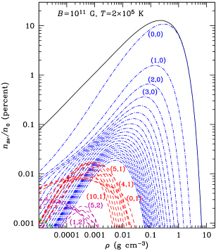
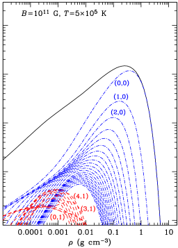
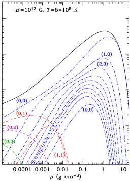
Figure 2: Fractional abundances of different nondissolved bound states $(s,\nu)$ with respect to the total number of electrons (free and bound), $n_{s\nu}/n_{0}$, as functions of mass density $\rho$, for $B=10^{11}$ G and $T=2\times 10^{5}$ K (left panel), $B=10^{11}$ G and $T=5\times 10^{5}$ K (middle panel), and $B=10^{12}$ G and $T=5\times 10^{5}$ K (right panel). The fractional abundances of tightly bound states ($\nu=0$) are plotted by dot-dashed lines, and loosely bound states ($\nu\geq 1$) by dashed lines. The solid lines show the total fractional abundance of the atoms that contribute to bound-bound and bound-free opacities.

Once the free energy is obtained, its derivatives over $\rho$ and $T$ and their combinations provide the other thermodynamic functions. However, the atomic partial number fractions $x_{s\nu}=n_{s\nu}/n_{0}$ that are evaluated in the course of the free energy minimization cannot be used directly to calculate opacities. At the considered conditions, interactions between different plasma particles give rise to a significant fraction of clusters. Such clusters contribute to the equation of state similarly to the atoms, lowering the pressure, but their radiation-absorption properties differ from those of an isolated atom. Therefore we should not count them in the fraction of atoms $x_{\mathrm{H}}$ that contribute to the bound-bound and bound-free opacities. Analogously, at low $\rho$ we should not include in $x_{\mathrm{H}}$ the highly excited states that do not satisfy the Inglis & Teller (1939) criterion of spectral line merging, being strongly perturbed by plasma microfields. Such states form the so called optical pseudo-continuum (e.g., Däppen et al. 1987). Thus, we discriminate between the atoms that keep their identity and the “dissolved” states that are strongly perturbed by the plasma environment. This distinction between the “thermodynamic” and “optical” neutral fractions is inevitable in the chemical picture of a plasma (see, e.g., Potekhin 1996, for discussion). The fraction of truly bound atoms is evaluated with the use of the occupation probability formalism. At every $s$, $\nu$, and $K_{\perp}$, we calculate the “optical” occupation probability $w_{s\nu}^{\mathrm{o}}(K_{\perp})$, replacing the Inglis-Teller criterion by an approximate criterion based on the average atomic size [Eq. (14) of Pavlov & Potekhin (1995)]. The fraction of weakly perturbed atoms, which contribute to the bound-bound and bound-free opacities, constitutes a fraction $w_{\nu s}^{\mathrm{o}}(K_{\perp})/w_{\nu s}(K_{\perp})<1$ of the total number of atoms. Here, $w_{\nu s}(K_{\perp})$ is the “thermodynamic” occupation probability derived from the free energy, which enters the generalized partition function (6).

Figure 2 illustrates the dependences of the fractional abundances of different weakly perturbed atomic states on $\rho$, $T$, and $B$. The left panel shows the case of $B=10^{11}$ G and relatively low temperature $T=2\times 10^{5}$ K. With increasing density, abundance of the bound states first increases at low $\rho$ according to the Saha equation and then decreases at higher $\rho$ because of pressure ionization. The middle panel demonstrates the case of a higher temperature $T=5\times 10^{5}$ K. In this case, all bound states are less abundant because of the thermal ionization. The right panel demonstrates the case of $T=5\times 10^{5}$ K and a stronger field, $B=10^{12}$ G. Here, the abundance of the atoms increases compared to the middle panel because of the larger binding energies. Pressure ionization starts at larger $\rho$, because the atomic sizes decrease with increasing $B$. The number of tightly bound states on the right panel is limited to ten ($0\leq s\leq 9$), the number of states with $\nu=1$ to two ($s=0,1$), and all states with $\nu\geq 2$ have $s=0$, because the states with nonzero $s$ and $\nu\geq 2$ are merged into continuum at $B=10^{12}$ G.

4 Polarization modes and opacities

4.1 Polarization modes

Propagation of radiation in magnetized plasmas was discussed in many papers and monographs (e.g., Ginzburg 1970). In coordinates with the $z$-axis along $\bm{B}$, the plasma dielectric tensor is (Ginzburg 1970)

$$\bm{\varepsilon}=\mathbf{I}+4\pi\bm{\chi}=\left(\begin{array}[]{ccc}\varepsilon_{\perp}&\mathrm{i}\varepsilon_{\wedge}&0\\ -\mathrm{i}\varepsilon_{\wedge}&\varepsilon_{\perp}&0\\ 0&0&\varepsilon_{\|}\end{array}\right),$$ (7)

where $\mathbf{I}$ is the unit tensor, $\bm{\chi}=\bm{\chi}^{\mathrm{H}}+\mathrm{i}\bm{\chi}^{\mathrm{A}}$ is the complex polarizability tensor of plasma, $\bm{\chi}^{\mathrm{H}}$ and $\bm{\chi}^{\mathrm{A}}$ are its Hermitian and anti-Hermitian parts, respectively. This tensor becomes diagonal, $\bm{\chi}=\textrm{diag}(\chi_{+1},\chi_{-1},\chi_{0})$, in the cyclic (or rotating) coordinates with unit vectors $\hat{\mathbf{e}}_{\pm 1}=(\hat{\mathbf{e}}_{x}\pm\mathrm{i}\hat{\mathbf{e}}_{y})/\sqrt{2}$, $\hat{\mathbf{e}}_{0}=\hat{\mathbf{e}}_{z}$.

At photon energies $\hbar\omega$ much higher than

$$\hbar\omega_{\mathrm{pl}}=\left(\frac{4\pi\hbar^{2}e^{2}n_{\mathrm{e}}}{m_{\mathrm{e}}}\right)^{1/2}=28.7\,\rho^{1/2}\mathrm{\leavevmode\nobreak\ eV},$$ (8)

where $\omega_{\mathrm{pl}}$ is the electron plasma frequency and $\rho$ is in g cm^-3, radiation propagates in the form of extraordinary (hereafter labeled by $j=1$) and ordinary ($j=2$) normal modes. These modes have different polarization vectors $\bm{e}_{j}$ and different absorption and scattering coefficients, which depend on the angle $\theta_{B}$ between the photon wave vector $\bm{k}$ and $\bm{B}$ (e.g., Kaminker et al. 1982). The two modes interact with each other via scattering. Gnedin & Pavlov (1974) formulated the radiative transfer problem in terms of these modes.

At a fixed photon frequency $\omega$, the absorption opacity $\kappa_{j}^{\mathrm{a}}(\theta_{B})$ in each mode $j$ and scattering opacities $\kappa_{jj^{\prime}}^{\mathrm{s}}(\theta_{B})$ from mode $j$ into mode $j^{\prime}$ can be presented as (e.g., Kaminker et al. 1982)

$$\kappa_{j}^{\mathrm{a}}(\theta_{B})=\frac{1}{m_{\mathrm{H}}}\sum_{\alpha=-1}^{1}|e_{j,\alpha}(\theta_{B})|^{2}\,\sigma_{\alpha}^{\mathrm{a}},$$ (9)

$$\kappa_{jj^{\prime}}^{\mathrm{s}}(\theta_{B})\!=\!\!{\frac{3}{4}}\!\!\sum_{\alpha=-1}^{1}\!\!|e_{j,\alpha}(\theta_{B})|^{2}\,\frac{\sigma_{\alpha}^{\mathrm{s}}}{m_{\mathrm{H}}}\int_{0}^{\pi}\!\!\!|e_{j^{\prime},\alpha}(\theta_{B}^{\prime})|^{2}\sin\theta_{B}^{\prime}\,\mathrm{d}\theta_{B}^{\prime},$$ (10)

where $\alpha=0,\pm 1$, $e_{j,0}=e_{j,z}$ and $e_{j,\pm 1}=(e_{j,x}\pm\mathrm{i}e_{j,y})/\sqrt{2}$ are the components of $\bm{e}_{j}$ in the cyclic coordinates. The cross sections $\sigma_{\alpha}$ depend on $\omega$ and $\alpha$, but not on $j$ or $\theta_{B}$. The total scattering opacity from mode $j$ is $\kappa_{j}^{\mathrm{s}}=\kappa_{j1}^{\mathrm{s}}+\kappa_{j2}^{\mathrm{s}}$, and the total extinction opacity is $\kappa_{j}=\kappa_{j}^{\mathrm{a}}+\kappa_{j}^{\mathrm{s}}$.

4.2 Scattering

Scattering cross-sections in neutron-star photospheres are well known (Ventura 1979; Kaminker et al. 1982; Mészáros 1992). For $\alpha=-1$, the photon-electron scattering has a resonance at $\omega_{\mathrm{ce}}$. Outside a narrow (about the Doppler width) frequency interval around $\omega_{\mathrm{ce}}$, the cross sections for the basic polarizations $\alpha=0,\pm 1$ are

$$\sigma_{\alpha}^{\mathrm{s,e}}=\frac{\omega^{2}}{(\omega+\alpha\omega_{\mathrm{ce}})^{2}+\nu_{\mathrm{e},\alpha}^{2}}\,\sigma_{\mathrm{T}},$$ (11)

where $\sigma_{\mathrm{T}}=({8\pi}/{3})({e^{2}}/{m_{\mathrm{e}}c^{2}})^{2}$ is the nonmagnetic Thomson cross section, and $\nu_{\mathrm{e},\alpha}$ are effective damping factors (see below).

The photon-ion scattering cross section looks analogously,

$$\sigma_{\alpha}^{\mathrm{s,i}}=\left(\frac{m_{\mathrm{e}}}{m_{\mathrm{p}}}\right)^{2}\frac{\omega^{2}}{(\omega-\alpha\omega_{\mathrm{cp}})^{2}+\nu_{\mathrm{i},\alpha}^{2}}\,\sigma_{\mathrm{T}}.$$ (12)

The resonance at $\omega_{\mathrm{cp}}$ due to the scattering on ions can be important in superstrong fields.

In each case, the damping factor $\nu_{\mathrm{e},\alpha}$ or $\nu_{\mathrm{i},\alpha}$ is equal to the half of the total rate of spontaneous and collisional decay of the state with energy $\hbar\omega$ (see discussion in Potekhin & Lai 2007). The spontaneous decay rates are

$$2\nu_{\mathrm{e}}^{\mathrm{s}}=\frac{4}{3}\,\frac{e^{2}}{m_{\mathrm{e}}c^{3}}\,\omega^{2},\quad 2\nu_{\mathrm{i}}^{\mathrm{s}}=\frac{4}{3}\,\frac{e^{2}}{m_{\mathrm{p}}c^{3}}\,\omega^{2}.$$ (13)

For the proton-electron plasmas, the damping factors that include the scattering and free-free processes can be approximately written as (Paper II)

$$\nu_{\mathrm{e},\alpha}=\nu_{\mathrm{e}}^{\mathrm{s}}+\nu_{\alpha}^{\mathrm{ff}}(\omega_{\mathrm{ce}}),\quad\nu_{\mathrm{e},\alpha}=\nu_{\mathrm{e}}^{\mathrm{s}}+(m_{\mathrm{e}}/m_{\mathrm{p}})\nu_{\alpha}^{\mathrm{ff}}(\omega_{\mathrm{cp}}),$$ (14)

where $\nu_{\alpha}^{\mathrm{ff}}(\omega)$ is the effective free-free frequency given by Eq. (17) below.

4.3 Absorption

4.3.1 Cyclotron absorption

Without magnetic field, absorption of a photon by a free electron is impossible without involvement of a third particle, which would accept the difference between the values of the total momentum of the electron and the photon before and after the absorption. In a quantizing magnetic field, a photon can be absorbed or emitted by a free electron in a transition between Landau levels. In the nonrelativistic or dipole approximation, such transitions occur between the neighboring levels at the frequency $\omega_{\mathrm{ce}}$. In the relativistic theory, the multipole expansion leads to an appearance of cyclotron harmonics (Zheleznyakov 1996). Absorption cross-sections at these harmonics were derived in the Born approximation by Pavlov et al. (1980) and represented in a compact form by Suleimanov et al. (2012).

4.3.2 Free-free absorption

The quantization of electron motion gives rise to cyclotron harmonics in the nonrelativistic theory. Pavlov & Panov (1976) derived photon absorption cross-sections for an electron, which moves in a magnetic field and interacts with a nonmoving point charge. This model is applicable at $\omega\gg\omega_{\mathrm{cp}}$. A more accurate treatment of absorption of a photon by the system of a proton and an electron yields (Paper II; Potekhin 2010)

$$\sigma_{\alpha}^{\mathrm{ff}}(\omega)=\frac{4\pi e^{2}}{m_{\mathrm{e}}c}\,\frac{\omega^{2}\,\nu_{\alpha}^{\mathrm{ff}}(\omega)}{(\omega+\alpha\omega_{\mathrm{ce}})^{2}(\omega-\alpha\omega_{\mathrm{cp}})^{2}+\omega^{2}\tilde{\nu}_{\alpha}^{2}(\omega)},$$ (15)

where $\nu_{\alpha}^{\mathrm{ff}}$ is an effective photoabsorption collision frequency and $\tilde{\nu}_{\alpha}$ is a damping factor. In the electron-proton plasma, taking into account the scattering and free-free absorption, we have (Paper II)

$$\tilde{\nu}_{\alpha}=(1+\alpha{\omega_{\mathrm{ce}}}/{\omega})\nu_{\mathrm{i},\alpha}(\omega)+(1-\alpha{\omega_{\mathrm{cp}}}/{\omega})\nu_{\mathrm{e},\alpha}(\omega)+\nu_{\alpha}^{\mathrm{ff}}(\omega).$$ (16)

We see from (15) that $\sigma_{-1}^{\mathrm{ff}}$ and $\sigma_{+1}^{\mathrm{ff}}$ have a resonance at the frequencies $\omega_{\mathrm{ce}}$ and $\omega_{\mathrm{cp}}$, respectively. The effective free-free absorption frequency can be written as

$$\nu_{\alpha}^{\mathrm{ff}}(\omega)=\frac{4}{3}\,\sqrt{\frac{2\pi}{m_{\mathrm{e}}T}}\,\frac{n_{\mathrm{e}}\,e^{4}}{\hbar\omega}\Lambda_{\alpha}^{\mathrm{ff}}(\omega),$$ (17)

where $\Lambda_{\alpha}^{\mathrm{ff}}(\omega)$ is a dimensionless Coulomb logarithm ($\Lambda_{\alpha}^{\mathrm{ff}}=(\pi/\sqrt{3})g_{\alpha}^{\mathrm{ff}}$, where $g_{\alpha}^{\mathrm{ff}}$ is a Gaunt factor). Without the magnetic field, $\Lambda_{\alpha}^{\mathrm{ff}}$ is a smooth function of $\omega$. In a quantizing magnetic field, however, it has peaks at the multiples of $\omega_{\mathrm{ce}}$ and $\omega_{\mathrm{cp}}$ for all polarizations $\alpha$. An accurate calculation of $\Lambda_{\alpha}^{\mathrm{ff}}(\omega)$ (Potekhin 2010) demonstrates that, unlike the electron cyclotron harmonics, the ion cyclotron harmonics are so weak that they can be safely neglected in the neutron-star atmosphere models.

In addition to the free-free absorption due to the electron-proton collisions, in Paper II we also considered the free-free absorption due to the proton-proton collisions. The results revealed that at $T\lesssim 10^{7}$ K and $\hbar\omega/T\lesssim 10$ the corresponding photoabsorption cross section is much smaller than the usual free-free absorption due to the proton-electron collisions, whereas at larger $\hbar\omega$ it is smaller than the scattering cross section. Therefore the proton-proton collisions can be neglected in the opacity calculations.

4.3.3 Bound-bound absorption

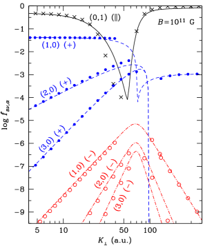
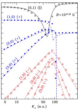
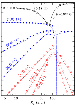
Figure 3: Analytical approximations (lines) and results of calculations (symbols) for oscillator strengths of transitions from the ground state to different bound states $(s,\nu)$ marked near the respective curves with absorption of a photon with polarization $\alpha=-1$ (dot-dashed lines and empty circles), $\alpha=0$ (solid lines and crosses), or $\alpha=+1$ (dashed lines and filled dots) at $B=10^{11}$ G (left panel), $3.16\times 10^{11}$ G (middle panel), and $10^{12}$ G (right panel).

Bound-bound transitions of the H atom moving in a strong magnetic field were studied by Pavlov & Potekhin (1995). In the dipole approximation, the cross section of an atom in a state $(s,\nu)$ for absorption of a photon with frequency $\omega$ and polarization $\alpha$ with a transition to a state $(s^{\prime},\nu^{\prime})$, averaged over the atomic states of motion, reads

$$\sigma_{\alpha;s\nu;s^{\prime}\nu^{\prime}}(\omega) = \frac{2\pi^{2}e^{2}}{m_{\mathrm{e}}c}\left(1-\mathrm{e}^{-\hbar\omega/T}\right)\frac{1}{A_{s\nu}}\int_{0}^{\infty}2\pi K_{\perp}\mathrm{d}K_{\perp}$$ (18)

$$\times\,w_{s\nu}^{\mathrm{o}}(K_{\perp})\exp(E_{s\nu}(K_{\perp})/T)$$

$$\times\,w_{s^{\prime}\nu^{\prime}}^{\mathrm{o}}(K_{\perp})f_{\alpha;s\nu;s^{\prime}\nu^{\prime}}(K_{\perp})\,\phi_{s\nu;s^{\prime}\nu^{\prime}}(K_{\perp},\Delta\omega),$$

where

$$A_{s\nu}=\int_{0}^{\infty}{2\pi K_{\perp}\mathrm{d}K_{\perp}w_{s\nu}^{\mathrm{o}}(K_{\perp})\exp(E_{s\nu}(K_{\perp})/T)}$$ (19)

is the normalization integral,

$$f_{\alpha;s\nu;s^{\prime}\nu^{\prime}}(K_{\perp})=\frac{\hbar\omega}{\mbox{Ry}}\,\left|\frac{\langle s^{\prime},\nu^{\prime},K_{\perp}|r_{-\alpha}|s,\nu,K_{\perp}\rangle}{a_{\mathrm{B}}}\right|^{2},$$ (20)

is the oscillator strength in the dipole approximation, $r_{0}=z$, $r_{\pm 1}=(x\pm\mathrm{i}y)/\sqrt{2}$,

$$\Delta\omega=\omega-\left[E_{s\nu}(K_{\perp})-E_{s^{\prime}\nu^{\prime}}(K_{\perp})\right]/\hbar,$$ (21)

and $\phi_{s\nu;s^{\prime}\nu^{\prime}}(K_{\perp},\Delta\omega)$ describes a normalized profile of the spectral line at a fixed $K_{\perp}$, $\int\phi_{s\nu;s^{\prime}\nu^{\prime}}(K_{\perp},\Delta\omega)\mathrm{d}\Delta\omega=1.$ The latter profile is assumed Lorentzian with width $\Gamma_{\alpha;s\nu;s^{\prime}\nu^{\prime}}(K_{\perp})$, determined by electron-atom collisions (see Pavlov & Potekhin 1995). In practice the collisional broadening plays minor role compared to the magnetic broadening due to the dependence of $\Delta\omega$ on $K_{\perp}$, except for stationary frequencies $\left[E_{s\nu}(K_{\perp})-E_{s^{\prime}\nu^{\prime}}(K_{\perp})\right]/\hbar$ for which $\mathrm{d}E_{s\nu}(K_{\perp})/\mathrm{d}K_{\perp}=\mathrm{d}E_{s^{\prime}\nu^{\prime}}(K_{\perp})/\mathrm{d}K_{\perp}$ – in particular, $\left[E_{s\nu}(K_{\perp})-E_{s^{\prime}\nu^{\prime}}(K_{\perp})\right]/\hbar$ at $K_{\perp}\to 0$, $(s^{\prime}-s)\omega_{\mathrm{cp}}$ at $K_{\perp}\to\infty$, and a small frequency corresponding to anticrossings at $K_{\perp}\sim K_{\mathrm{c}}$. The magnetic broadening exceeds by orders of magnitude the usual Doppler broadening, which allows us to neglect the difference between the pseudomomenta in the initial and final states in Eqs. (18) and (20). The spectral profile of the bound-bound opacities becomes continuous in a wide frequency range, resembling a reversed bound-free profile. We calculate the integral (18) using analytical approximations for the electron collision widths $\Gamma_{\alpha;s\nu;s^{\prime}\nu^{\prime}}(K_{\perp})$ suggested in Potekhin (1998) and the approximations for binding energies $E_{s\nu}(K_{\perp})$ and oscillator strengths $f_{\alpha;s\nu;s^{\prime}\nu^{\prime}}(K_{\perp})$ presented in the Appendix.

Examples of the oscillator strengths are shown in Fig. 3, where the results of numerical calculations by the method described in Potekhin (1994) are compared with the analytical approximations (Appendix A.3). The figure shows oscillator strengths for the main dipole-allowed transitions from the ground state to excited discrete levels as functions of $K_{\perp}$. Since the atomic wave functions are symmetric with respect to the $z$-inversion for the states with even $\nu$, and antisymmetric for odd $\nu$, only the transitions that change the parity of $\nu$ are allowed for the polarization along the field ($\alpha=0$), and only those preserving the parity for the circular polarizations ($\alpha=\pm 1$). For an atom at rest, in the dipole approximation, due to the conservation of the $z$-projection of the total angular momentum of the system, absorption of a photon with polarization $\alpha$ results in the change of $s$ by $\alpha$. This selection rule for a nonmoving atom manifests itself in vanishing oscillator strengths at $K_{\perp}\to 0$ for $s\neq\alpha$. In an appropriate coordinate system (Burkova et al. 1976; Potekhin 1994), the symmetry is restored at $K_{\perp}\to\infty$, therefore the transition with $s=\alpha$ is the only one that survives also in the limit of large pseudomomenta. But in the intermediate region of $K_{\perp}$, where the transverse atomic velocity is not small, the cylindrical symmetry is broken, so that transitions to other levels are allowed. For this reason the corresponding oscillator strengths in Fig. 3 have maxima at $K_{\perp}\sim K_{\mathrm{c}}$.

4.3.4 Bound-free absorption

The theory of photoionization of the H atom in a strong magnetic field with allowance for motion and a method of calculation of the cross sections was described by Potekhin & Pavlov (1997), who adapted the $R$-matrix formalism (Wigner & Eisenbud 1947; Seaton 1983) to the case under study. Since this numerical treatment is computationally involved, we first compose a set of tables of the photoionization cross sections $\sigma_{\alpha;s\nu}^{\mathrm{bf}}(\omega,K_{\perp})$, and then calculate the bound-free opacities using interpolation across these tables. At a given $B$, for each of the three basic polarizations $\alpha$, we calculate $\sigma_{\alpha;s\nu}^{\mathrm{bf}}(\omega,K_{\perp})$ on a predefined grid, as in Papers II and III. Now we have refined the grid in photon energy, with $\log_{10}\hbar\omega\ [\mathrm{eV}]$ ranging from 0 to 5 with step 0.01, and modified the grid of $\log_{10}K_{\perp}$. In order to avoid large numerical errors due to strong coupling of the orbitals at $K_{\perp}\sim K_{\mathrm{c}}$, we exclude a range of $K_{\perp}$ around $K_{\mathrm{c}}$ and use two separate grids for $K_{\perp}$ below and above the excluded region. Each of these grids has, as previously, an equal step in $\log K_{\perp}$. The size of the excluded region is determined ad hoc, from numerical tests at different $K_{\perp}$ values. The employed modification of the grid is justified by a comparison of the results in the overlap range of $B\sim 10^{12}$ G, which reveals virtually no difference between the opacities calculated with the old and new tables of the bound-free cross sections.

As in Papers II and III, we filter out spurious outliers, which appear because of the Beutler-Fano resonances, whose widths are smaller than the step of our grid in $\log\omega$, using the 3-point median filter at every $K_{\perp}$. The photoionization threshold is determined independently for every $K_{\perp}$, using the analytic fits to the binding energies given in Appendix A.1.

In addition to the bound-bound and bound-free atomic transitions, in a plasma environment there are transitions from bound states to the highly perturbed atomic states discussed in Sect. 3. These perturbed levels effectively dissolve and merge in a pseudo-continuum, which lies below the photoionization threshold. In order to take into account the radiative transitions into this pseudo-continuum, we employ a technique of below-threshold extrapolation, which is usual in the zero-field case (Däppen et al. 1987; Stehlé & Jacquemot 1993; Seaton et al. 1994). The details of this technique for the case of an atom moving in a strong magnetic field are given in Paper II. As previously, the precalculated, filtered and extrapolated photoionization cross sections are averaged over $K_{\perp}$ with statistical weights $w_{s\nu}^{\mathrm{o}}(K_{\perp})\exp[E_{s\nu}(K_{\perp})/T]$.

4.4 Polarization vectors

In the coordinate system $(x^{\prime},y^{\prime},z^{\prime})$ rotated with respect to $(x,y,z)$ so that $z^{\prime}$ is along the wave vector $\bm{k}$ and $\bm{B}$ is in the $(x^{\prime},z^{\prime})$ plane, the electromagnetic polarization vectors $\bm{e}_{j}$ (Sect. 4.1) can be written as (Ho & Lai 2001, 2003)

$$(e_{j,x},e_{j,y},e_{j,z})=(1+K_{j}^{2}+K_{z,j}^{2})^{-1/2}\,(iK_{j},1,iK_{z,j}),$$ (22)

where

$$K_{j}=\beta\left\{1+(-1)^{j}\left[1+\frac{1}{\beta^{2}}+\frac{m}{1+{a}}\frac{\sin^{2}\theta_{B}}{\beta^{2}}\right]^{1/2}\right\},$$ (23)

$$K_{z,j}=-\frac{(\varepsilon_{\perp}^{\prime}-\varepsilon_{\|}^{\prime})K_{j}\cos\theta_{B}+\varepsilon_{\wedge}}{\varepsilon_{\perp}^{\prime}\sin^{2}\theta_{B}+\varepsilon_{\|}^{\prime}\cos^{2}\theta_{B}}\,\sin\theta_{B},$$ (24)

$$\beta=\frac{\varepsilon_{\|}^{\prime}-\varepsilon_{\perp}^{\prime}+\varepsilon_{\wedge}^{2}/\varepsilon_{\perp}^{\prime}+\varepsilon_{\|}^{\prime}\,{m}/(1+{a})}{2\,\varepsilon_{\wedge}}\,\,\frac{\varepsilon_{\perp}^{\prime}}{\varepsilon_{\|}^{\prime}}\,\,\frac{\sin^{2}\theta_{B}}{\cos\theta_{B}},$$ (25)

$$\varepsilon_{\perp}^{\prime}=\varepsilon_{\perp}+{a},\qquad\varepsilon_{\|}^{\prime}=\varepsilon_{\|}+{a}+{q}.$$

Here, the parameters $K_{j}$ and $K_{z,j}$ are expressed in terms of the complex dielectric tensor of a plasma (7), dielectric tensor of vacuum $4\pi\bm{\chi}^{\textrm{vac}}=\textrm{diag}({a},{a},{a}+q)$, and the inverse magnetic permeability of the vacuum $\bm{\mu}^{-1}=\mathbf{I}+\textrm{diag}({a},{a},{a}+m)$. We calculate the plasma dielectric tensor using the relation between the polarizability coefficients $\chi_{\alpha}$ and the opacities (Potekhin et al. 2004)

$${\chi}^{\mathrm{H}}_{\alpha}(\omega) = \frac{c\rho}{4\pi^{2}\omega}\,\bigg{\{}\!\int_{0}^{\omega}\!\big{[}\,\kappa_{\alpha}(\omega+\omega^{\prime})-\kappa_{\alpha}(\omega-\omega^{\prime})\,\big{]}\frac{\mathrm{d}\omega^{\prime}}{\omega^{\prime}}$$ (26)

$$+ \int_{2\omega}^{\infty}\frac{\kappa_{\alpha}(\omega^{\prime})}{\omega^{\prime}-\omega}\,\mathrm{d}\omega^{\prime}-\int_{0}^{\infty}\frac{\kappa_{-\alpha}(\omega^{\prime})}{\omega^{\prime}+\omega}\,\mathrm{d}\omega^{\prime}\bigg{\}}.$$

The vacuum polarizability and permeability coefficients ${a}$, $q$, and $m$ can be neglected at the relatively weak field strengths considered here, but in general they have been fitted by elementary functions (Potekhin et al. 2004).

5 Atomic signatures in the opacities and spectra

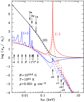
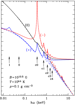
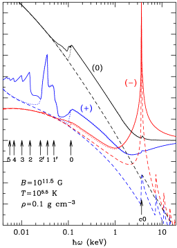
Figure 4: Logarithms of total basic cross sections $\sigma_{\alpha}$ (solid lines), $\alpha=-1,0,+1$ marked “($-$)”, “(0)”, and ”(+)”, respectively. For comparison, the logarithms of cross sections without contribution of excited bound states (dotted lines) and free-free cross sections$\sigma_{\alpha}^{\mathrm{ff}}$ (dashed lines) are plotted. The three panels correspond to three sets of plasma parameters $\rho$, $T$, and $B$ marked on the plots. The arrows correspond to different characteristic transition energies for a nonmoving H atom (see text for discussion): 0 – $E_{0,0}$ (the principal photoionization threshold), 1 – $(E_{0,0}-E_{1,0})$, $1^{\prime}$ – $(E_{0,0}-E_{2,0})$, $1^{\prime\prime}$ – $(E_{0,0}-E_{3,0})$, 2 – $(E_{1,0}-E_{2,0})$, $2^{\prime}$ – $(E_{1,0}-E_{3,0})$, 3 – $(E_{2,0}-E_{3,0})$, 4 – $(E_{3,0}-E_{4,0})$, 5 – $(E_{4,0}-E_{5,0})$; 1a – $(E_{0,0}-E_{0,1})$, 2a – $(E_{1,0}-E_{1,1})$, 3a – $(E_{2,0}-E_{2,1})$. The arrows marked c0, c1, c2, c3, c4 correspond to cyclotron harmonics energies $(N+1)\hbar\omega_{\mathrm{ce}}$ with $N=0,1,2,3,4$, respectively.

5.1 Basic opacities

Figure 4 shows examples of the basic cross sections $\sigma_{\alpha}$ in Eqs. (9), (10) at $T=3.16\times 10^{5}$ K and different values of $B$ and $\rho$. The left panel shows the case of $B=3.16\times 10^{10}$ G and relatively low density $\rho=10^{-3}$ g cm^-3. In this case, the number fraction of the atoms is small, $x_{\mathrm{H}}=0.0025$. Nevertheless, we observe prominent absorption features due to bound-bound transitions between the neighboring tightly-bound states $(s-1,0)\to(s,0)$ ($s=1,2,3,4$ marked in the figure), which are allowed in the dipole approximation for $\alpha=+1$ for a nonmoving atom. The lines marked $1^{\prime}$ and $2^{\prime}$ correspond to the transitions $(s-1,0)\to(s+1,0)$ ($s=1,2$), which are dipole-forbidden for an atom at rest, but become noticeable for moving atoms. Since the energy difference between the initial and final levels is smaller at $K_{\perp}\neq 0$ than at $K_{\perp}=0$ (cf. Fig. 1), the maxima of the spectral lines are shifted to the left from the corresponding arrows in the figure, which are plotted at $\hbar\omega=E_{s+1,0}(0)-E_{s-1,0}(0)$. For the longitudinal polarization $\alpha=0$, there are narrow spikes, marked 1a, 2a, 3a, to the left of the energy $E_{00}(0)$, which are due to the transitions from the tightly-bound states to the lowest loosely-bound states of the same $s$-manifold, $(s,0)\to(s,1)$, with $s=0,1,2$, respectively. At higher energies, we see the peaks marked c0, c1, c2, c3 at the dashed curves. They are due to the absorption at the cyclotron fundamental frequency $\omega_{\mathrm{ce}}$ and its harmonics. The harmonics are not seen, however, in the total cross sections (solid lines in the left panel), because they are dominated by scattering at these energies and plasma parameters.

The quantum cyclotron harmonics become visible in the total cross sections at higher density $\rho=0.1$ g cm^-3 (the middle panel), because of the larger free-free absorption. Although the abundance of the atoms is also larger, $x_{\mathrm{H}}=0.021$, the atomic absorption features are merged into the free-free continuum. The absorption features due to transitions between neighboring tightly-bound states reappear at a stronger field $B=3.16\times 10^{11}$ G (the right panel), partly because of a higher abundance of the atoms ($x_{\mathrm{H}}=0.053$), but mainly because of the lowering of the continuum level for $\alpha=-1$ with increasing $B$. In the latter case, the cyclotron-absorption harmonics are again submerged under the scattering. The signatures of bound-bound transitions with absorption of a photon polarized along $\bm{B}$ ($\alpha=0$) are not visible in the middle and right panels, because the loosely-bound states are destroyed by pressure ionization and form quasicontinuum at this density.

The ground-state photoionization jump above the free-free continuum at $\hbar\omega=E_{00}$ is small at $B=3.16\times 10^{10}$ G in the left panel of Fig. 4 and virtually absent in the middle panel, because the product $x_{\mathrm{H}}\sigma_{\alpha}^{\mathrm{bf}}$ is smaller than $\sigma_{\alpha}^{\mathrm{ff}}$ in these cases. However, it is clearly visible at the higher field strength (the right panel). This jump is smoothed by the magnetic broadening and by photoionization of excited tightly-bound states, as seen from a comparison with the model where the excited states are neglected, which is plotted by the dotted lines.

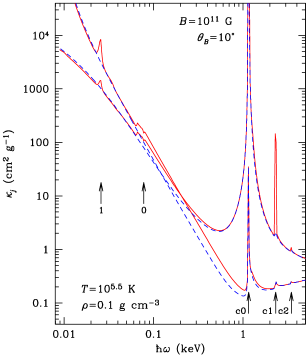
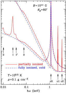
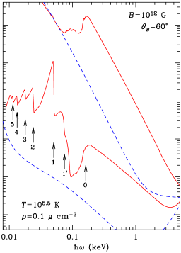
Figure 5: Opacities $\kappa_{j}$ of the normal polarization modes $j=1,2$ (the lower and upper curve of each type, respectively) in a magnetized plasma at $\rho=0.1$ g cm^-3 and $T=10^{5.5}$ K, for $B=10^{11}$ G and $\theta_{B}=10^{\circ}$ (left panel), $B=10^{11}$ G and $\theta_{B}=60^{\circ}$ (middle panel), and $B=10^{12}$ G and $\theta_{B}=60^{\circ}$ (right panel). Accurate opacities (solid lines) are compared with the approximation of the cold, fully ionized plasma (dashed lines). The arrows correspond to different characteristic transition energies and are marked in the same way as in Fig. 4.

5.2 Opacities for the normal modes

The basic opacities obtained in Sect. 5.1 have been used to calculate plasma polarizabilities and polarization vectors of the normal modes (Sect. 4.4).

Figure 5 illustrates the effect of incomplete ionization on the opacities for the two normal modes (Sect. 4.1). Here, the atomic features analogous to those in Fig. 4 are also seen. The features marked by numbers 2 through 5 arise from the bound-bound radiative transitions from excited tightly bound states, which were not included in the previous opacity calculations (Potekhin et al. 2004). In addition to the bound-bound, bound-free, and free-free absorption, we have also included the cyclotron absorption beyond the cold plasma approximation, following Suleimanov et al. (2012). The latter absorption gives rise to the high and narrow peaks, marked “c1” and “c2” in the left and middle panels. These peaks correspond to the synchrotron harmonics (Zheleznyakov 1996) and thus they present a manifestation of an effect of special relativity. For comparison, we plot by dashed lines the opacities calculated in the approximation of cold, fully ionized plasma. In the latter approximation, the atomic features are absent because of the full ionization, and the peaks at the cyclotron harmonics are much smaller. The latter difference demonstrates that, despite the smallness of the relativistic parameters $T/m_{\mathrm{e}}c^{2}$ and $\hbar\omega_{\mathrm{ce}}/m_{\mathrm{e}}c^{2}$, the relativistic effects substantially change the opacities at the cyclotron harmonics frequencies, in agreement Suleimanov et al. (2012).

Figures 4 and 5 show that photoionization becomes substantial at relatively strong magnetic fields. The contribution of the bound-bound transitions into the opacities also increases with field increase, but the bound-free absorption grows faster and becomes more important. This tendency continues at higher fields, so that the bound-bound transitions becomes unimportant for magnetars, at contrast to the bound-free ones (Paper III).

5.3 Spectra

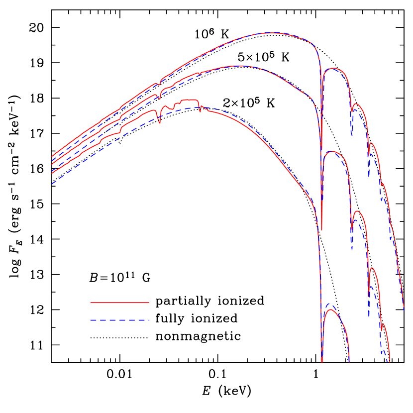
Figure 6: The local spectrum of a neutron star with magnetic field $B=10^{11}$ G, normal to the surface, and with effective temperatures $T_{\mathrm{eff}}=10^{6}$ K, $5\times 10^{5}$ K, and $2\times 10^{5}$ K (marked near the curves). The partially ionized atmosphere spectrum (solid lines) is compared with the fully ionized atmosphere model (dashed lines) and with the nonmagnetic atmosphere model (dotted lines).

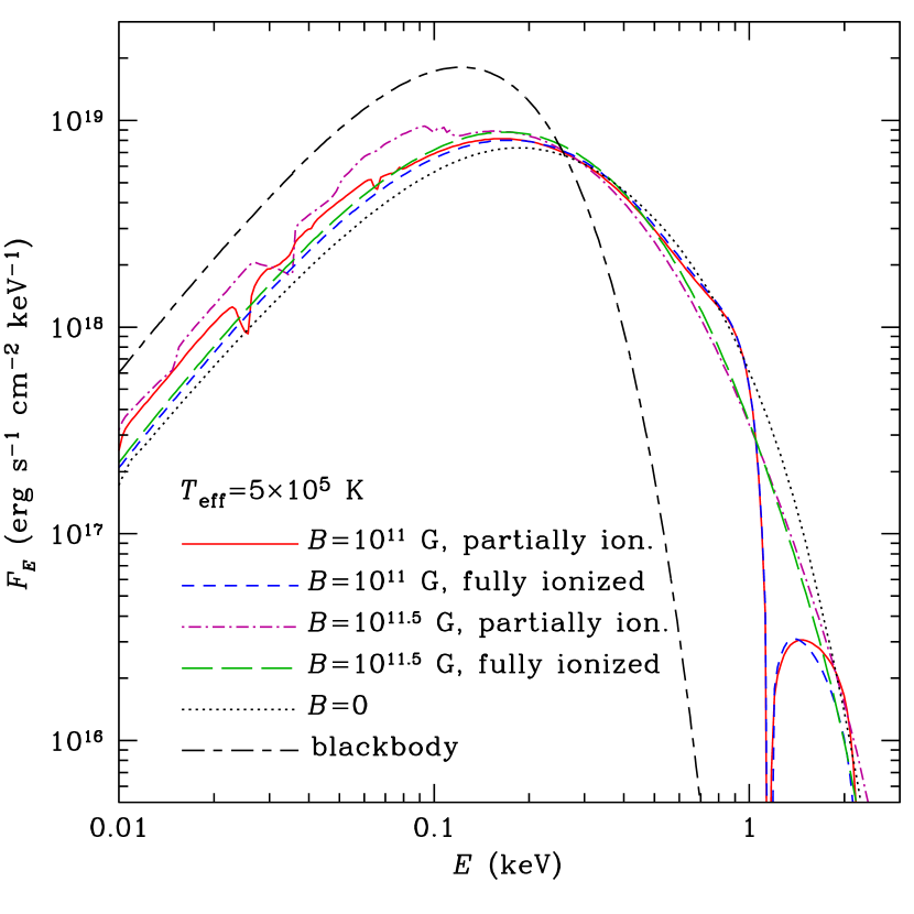
Figure 7: The local spectrum of a partially ionized atmosphere of a neutron star with effective temperature $T_{\mathrm{eff}}=5\times 10^{5}$ K, with magnetic fields $B=3.16\times 10^{11}$ G (dot-dashed line), $10^{11}$ G (solid line) and 0 G (dotted line). Blackbody spectrum (short-long-dashed line) and spectra of a magnetized, but fully ionized, atmosphere are also shown.

We have included the calculated opacities in the equations of radiative transfer for the two normal modes and solved it numerically with the equations of hydrostatic and energy balance, using the numerical method developed by Ho & Lai (2001). Examples of the resulting atmosphere spectra are shown in Figs. 6 and 7.

Figure 6 shows a spectrum of a neutron star with magnetic field $B=10^{11}$ G and effective temperatures $T_{\mathrm{eff}}=10^{6}$ K, $5\times 10^{5}$ K, and $2\times 10^{5}$ K, calculated using the models of fully and partially ionized hydrogen atmospheres. In these examples, we assumed gravity $g=2\times 10^{14}$ cm s^-2, which corresponds, for example, to a neutron star with mass $M=1.4\,M_{\odot}$ and radius $R=10.9$ km. For realistic neutron-star equation of state BSk21 (Goriely et al. 2010; Potekhin et al. 2013), this $g$ corresponds to $M=1.8\,M_{\odot}$ and $R=12.5$ km. The first and second values of the effective temperatures fall in the range of current observational estimates for a number of thermally emitting neutron stars (Viganò et al. 2013), albeit the hot spots observed on CCOs have $T>10^{6}$ K. The third value, $T_{\mathrm{eff}}=2\times 10^{5}$ K, has not been observed. Indeed, thermal radiation of such cold neutron star is difficult to measure because of the low thermal flux. However, this value of $T_{\mathrm{eff}}$ is also plausible, and if there are such neutron stars at distances within $\sim 100$ pc, their thermal spectra may be measured in the future. For the partially ionized models with $T_{\mathrm{eff}}\geq 5\times 10^{5}$ K, one can notice the absorption feature at $E=26$ eV, which corresponds to the transition between the ground state and the lowest excited state of the H atom, but otherwise the spectrum is smooth and close to the one in the fully ionized plasma model. The atomic features are rather small and less significant than the cyclotron harmonics. At $T_{\mathrm{eff}}=2\times 10^{5}$ K, more atomic spectral features are discernible. At this field strength, they lie at rather low energies $E\lesssim 0.1$ keV.

Figure 7 presents a comparison of the spectra for $B=10^{11}$ G and $3.2\times 10^{11}$ G at $T_{\mathrm{eff}}=5\times 10^{5}$ K, calculated using the models of fully and partially ionized hydrogen atmosphere. At the stronger field, the atomic absorptions make a noticeable contribution to the spectrum at energies $\hbar\omega\sim 10$ – 100 eV, but even in this case they are not well pronounced. We conclude that the atomic absorption is not very important for the atmosphere spectra at $B\lesssim 10^{11}$ G, provided that $T_{\mathrm{eff}}\gtrsim 5\times 10^{5}$ K.

In Figs. 6 and 7 we also show the spectra in the model of partially ionized nonmagnetic H atmosphere (for details of this calculation, see Ho & Heinke 2009). In the latter model, there is no cyclotron lines, atomic absorption features are very weak (barely discernible) because of a high degree of plasma ionization, and the spectral maximum is shifted to higher energies by $\sim 10\%$ compared with the case of $B=10^{11}$ G. For comparison, in Fig. 7 we plot the blackbody model, which strongly underestimates the peak energy and overestimates the peak flux.

6 Conclusions

We have developed new analytical approximations for energies, sizes, and oscillator strengths of a H atom moving arbitrarily in moderately strong magnetic field $3\times 10^{10}\mbox{\leavevmode\nobreak\ G}\lesssim B\lesssim 10^{12}$ G. Using these approximations and extensive numerical calculations of the bound-free absorption cross sections, we calculated the ionization equilibrium, equation of state, and opacities at the moderate fields. The tables of the thermodynamic functions, atomic fractions, and Rosseland opacities, previously available online for $B=10^{12}$ – $10^{15}$ G (Papers I and II), are supplemented by the field interval $B=3\times 10^{10}$ – $10^{12}$ G.

The calculated spectral opacities are implemented in calculations of the neutron-star atmosphere models. The results show that at $B\ll 10^{12}$ G and $T_{\mathrm{eff}}\gtrsim 5\times 10^{5}$ K the atomic absorption features in the spectra are small. Bound-bound features at such field strengths are more significant than bound-free ones, but they occur at low energies, which are difficult to observe. Moreover, the distribution of the magnetic field over the surface should additionally smear these features and make them less significant, as has been demonstrated in the case of the stronger fields by Ho et al. (2008). On the other hand, despite the smallness of the characteristic thermal and photon energies compared to the electron rest energy, the relativistic cyclotron harmonics are clearly visible in the spectra at these field strengths, in agreement with the results previously reported by Suleimanov et al. (2012) and Ho (2013).

Appendix A Analytical approximations for atomic energies, sizes, and oscillator strengths

A.1 Binding energies

For the tightly bound states of a nonmoving H atom (any $s$, $\nu=0$, $K_{\perp}=0$), we use the analytical approximations for binding energies from Potekhin (2014). For the loosely bound states of a nonmoving H atom ($\nu\geq 0$, $K_{\perp}=0$), we use the analytical approximations from Potekhin (1998). Both sets of approximations are valid for many quantum states at $\gamma\gtrsim 1$.

For moving atoms ($K_{\perp}>0$) we use different approximations for the centered states, $E_{s\nu}^{(<)}(K_{\perp})$, and decentered states, $E_{s\nu}^{(>)}(K_{\perp})$, and replace the inflection point at $K_{\mathrm{c}}$ by the intersection of these two functions. For the centered states, we use Eq. (2) with

$$m_{s\nu}=m_{\mathrm{H}}\,[1+(\gamma/\gamma_{s\nu})^{p_{s\nu}}]$$ (27)

where $\gamma_{s\nu}$ and $p_{s\nu}$ are dimensionless parameters, which are approximated as functions of $s$ and $\nu$:

$$\gamma_{s0}=6\times 10^{3}/(1+2s)^{2},\quad p_{s0}=0.9,$$

$$\gamma_{s\nu}=\frac{110}{n^{2}\,(2-s+s^{2})},\quad n=\frac{\nu+1}{2},\quad p_{s\nu}=1.65\quad(\mbox{odd\leavevmode\nobreak\ }\nu),$$

$$\gamma_{s\nu}=\frac{55}{n^{2}\,(1+s+s^{2})},\quad n=\frac{\nu}{2},\quad p_{s\nu}=1.2\quad(\mbox{even\leavevmode\nobreak\ }\nu\geq 2).$$

For the decentered states with $\nu=0$, we use Eq. (3) with

$$\epsilon_{s0}=\hat{r}_{*}/(5+3s)+(2\mbox{Ry}/E_{s0}^{\|})^{2}.$$ (28)

For the decentered states with $\nu\geq 1$, we find that the formulae used previously for the binding energies at any $K_{\perp}$ for $\gamma>300$ (Potekhin 1998) remain valid at smaller $\gamma$ for $K_{\perp}>K_{\mathrm{c}}$.

These approximations are sufficiently accurate for modeling neutron star photospheres. The differences between neighboring energy levels are determined by these formulae with an accuracy of a few percent (except the $K_{\perp}$ ranges near anticrossings) at $10\lesssim\gamma\lesssim 1000$. Examples of calculated and fitted binding energies are shown in Fig. 1.

A.2 Atomic sizes

For the centered states, the electron cloud is cylindrically symmetric at $\gamma\gg 1$, except for the ranges of $K_{\perp}$ near level anticrossings. The root-mean-square (rms) sizes of this cloud transverse to the magnetic field are

$$l_{x}=l_{y}=a_{\mathrm{B}}\,\sqrt{(s+1)/\gamma},\quad l_{\perp}=a_{\mathrm{B}}\,\sqrt{2(s+1)/\gamma}.$$ (29)

The atomic size along the field is given at $K_{\perp}=0$ by the approximation (Potekhin 1998)

$$l_{z}^{(0)}=\frac{a_{\mathrm{B}}}{\sqrt{2}}+\frac{a_{\mathrm{B}}}{\ln[\gamma/(1+s)]}\,\frac{\mbox{Ry}}{E_{s0}^{\|}(0)}\quad(\nu=0),$$ (30)

$$l_{z}^{(0)}=1.6\,a_{\mathrm{B}}(\mbox{\leavevmode\nobreak\ Ry}/E_{s\nu}^{\|}(0))\quad(\nu\geq 1).$$ (31)

This size remains almost constant for the centered states of a moving atom. For the decentered states ($K_{\perp}>K_{\mathrm{c}}$), our approximation of the longitudinal size reads

$$l_{z}=\left[a_{\mathrm{B}}^{2}\left(\nu+1/2\right)\sqrt{\hat{r}_{*}^{3}+(4.3+7\nu^{2})\,\hat{r}_{*}^{2}}+\left(l_{z}^{(0)}\right)^{2}\right]^{1/2}$$ (32)

Unlike the case of $\gamma>300$ (Potekhin 1998), at smaller $\gamma$ we do not smooth the transition between Eq. (31) and Eq. (32).

Although the electron cloud is mostly cylindrically symmetric, the atom is not, because the proton and electron are not centered at the same axis. The atom acquires a constant dipole moment proportional to the mean electron-proton separation $\bar{x}$, which is considerably smaller than $r_{*}$ for the tightly bound states at $K_{\perp}<K_{\mathrm{c}}$ and approaches $r_{*}$ for the loosely bound or decentered states. At $\gamma\gtrsim 10$, the fractional difference between $\bar{x}$ and $r_{*}$ can be approximately described by expressions

$$1-\frac{\bar{x}}{r_{*}}=\left\{\begin{array}[]{l}\displaystyle\frac{1}{1+0.0014(1+s)^{2}\,\gamma^{0.77}}\quad(\nu=0,\leavevmode\nobreak\ K_{\perp}<K_{\mathrm{c}}),\\[12.91663pt] \displaystyle\frac{1}{1+(\gamma/55)^{3/2}}\quad(\nu=1,2,\leavevmode\nobreak\ K_{\perp}<K_{\mathrm{c}}),\\[12.91663pt] \displaystyle\left(\frac{17\ln(1+\gamma)\,(1-(1.5+2s)^{-1})}{\gamma\hat{r}_{*}}\right)^{3}\leavevmode\nobreak\ \leavevmode\nobreak\ \leavevmode\nobreak\ (\nu=0,\leavevmode\nobreak\ K_{\perp}>K_{\mathrm{c}}),\\[12.91663pt] 0\quad\mbox{otherwise.}\end{array}\right.$$ (33)

Then the total rms size that is used for calculation of the occupation probabilities (Paper I) is given by $\left(\bar{x}^{2}+l_{x}^{2}+l_{y}^{2}+l_{z}^{2}\right)^{1/2}.$

A.3 Oscillator strengths

In this section we present analytical approximations to the oscillator strengths $f_{\alpha;s\nu;s^{\prime}\nu^{\prime}}(K_{\perp})$, discussed in Sect. 4.3.3. It is sufficient to retain only the transitions with $\nu^{\prime}=\nu\pm 1$ for $\alpha=0$ and with $\nu^{\prime}=\nu$ for $\alpha=\pm 1$, because the other oscillator strengths are very small due to the smallness of the wave-function overlap integral implied in the matrix element in Eq. (20). As can be seen in Fig. 2, the loosely-bound states are populated very weakly compared to the tightly bound states, therefore we can restrict the consideration by initial states with $\nu=0$. Furthermore, the symmetry relation $f_{\alpha;s\nu;s^{\prime}\nu^{\prime}}=f_{-\alpha;s^{\prime}\nu^{\prime};s\nu}$ allows us to consider only the cases where $s^{\prime}\geq s$. Thus we are left with oscillator strengths $f^{(\alpha)}_{s,\Delta s}=f_{\alpha;s,0;s+\Delta s,0}$ for $\alpha=\pm 1$ and $f^{(0)}_{s}=f_{0;s,0;s,1}$ for $\alpha=0$.

In the dipole approximation for the nonmoving atom, the only nonzero oscillator strengths are those with $s^{\prime}=s+\alpha$. The corresponding oscillator strengths can be approximated as

$$f^{(0)}_{s}(0) = \left(1-\frac{0.584}{1+2.64\,\gamma^{1.076}}\right)\,\frac{1+6\times 10^{-6}\,\gamma}{1+0.247\gamma^{0.381}},$$ (34)

$$f^{(1)}_{s,1}(0) = \left(1-\frac{0.584}{1+12\gamma^{1.43}}\right)\,\frac{1+9.8\times 10^{-5}(s+1)\gamma}{1+1.585\gamma^{0.713}}$$ (35)

$$\qquad\times\,[1+2s/(1+\gamma/30)]^{-1/4}.$$

Equation (34) reproduces Eq. (21) of Potekhin (1998), but with a fixed typo, and Eq. (35) additionally generalizes it to nonzero $s$.

For the moving atom and $\alpha=\pm 1$, we keep only transitions with $\Delta s=s^{\prime}-s<4$, because the oscillator strengths strongly decrease with increasing $\Delta s$. First we define a field-dependent characteristic scale of $K_{\perp}$,

$$K_{1}=42.9\,[1+\gamma/2.4+(\gamma/84)^{2}+(\gamma/380)^{3}]^{0.17}m_{\mathrm{e}}e^{2}/\hbar.$$ (36)

Then our approximation for the longitudinal polarization reads

$$f^{(0)}_{s}(K_{\perp}) = f^{(0)}_{s}(0)\exp\left[-(c_{1}K_{\perp}/K_{1})^{2}\right]+\frac{\exp[-(c_{2}K_{\perp}/K_{1})^{-c_{3}}]}{1+0.5\sqrt{K_{1}/K_{\perp}}},$$

where

$$c_{1}=\frac{4}{1+\gamma/1200},\quad c_{2}=\frac{0.89}{1+\gamma/10^{4}},\quad c_{3}=\max(1,10-\ln\gamma).$$

For the main transition with circular polarization, viz. $\alpha=\Delta s=1$, first we introduce two functions describing $f^{(1)}_{s,1}(K_{\perp})$ at small and large $K_{\perp}$, respectively,

$$f^{(<)}_{s}(K_{\perp}) = 1-p_{1}\,(K_{\perp}/K_{1})^{2},\quad p_{1}=(1+\gamma/800)^{-1/2},$$

$$f^{(>)}_{s}(K_{\perp}) = 2(s+1)\frac{m_{\mathrm{e}}}{m_{\mathrm{p}}}\left[1-p_{1}\,(K_{1}/K_{\perp})^{2}\right],$$

and truncate (replace by 0) the negative values of these functions. At any $K_{\perp}$, our approximation reads

$$f^{(1)}_{s,1}(K_{\perp})=f^{(<)}_{s}(K_{\perp})\,X(K_{\perp})+f^{(>)}_{s}(K_{\perp})\,\big{[}1-X(K_{\perp})\big{]},$$ (38)

where

$$X(K_{\perp})=\frac{1}{1+(K_{\perp}/K_{1})^{p}},\quad p=\frac{83}{1+[\ln(1+\gamma/90)]^{2}}.$$ (39)

The oscillator strengths for the other considered transitions are

$$f^{(1)}_{s,\Delta s}(K_{\perp}) = p_{s,\Delta s}(K_{\perp}/K_{1})^{2\Delta s-2}\max(0,1-qK_{\perp}/K_{1}),$$ (40)

$$q = 0.72+0.12\ln(1+\gamma/400),$$

$$p_{s,2} = \frac{0.012\,[1+2s/(1+\gamma/30)]^{3/4}}{1+(\gamma/320)^{3/4}},$$

$$p_{s,3} = 0.0016+\frac{0.0055}{1+(19/\gamma)^{1.8}+(\Gamma/1270)^{4}},$$

$$f^{(-1)}_{s,\Delta s}(K_{\perp}) = \frac{p^{\prime}_{s,\Delta s}(K_{\perp}/K_{1})^{2\Delta s+2}}{1+p^{\prime\prime}_{s,\Delta s}(K_{\perp}/K_{1})^{5\Delta s+5}},$$ (41)

$$p^{\prime}_{s,1} = \frac{5\times 10^{-5}}{1+110/\gamma}\,\left[1+\frac{2s}{1+\gamma/40}\right]^{2},$$

$$p^{\prime}_{s,3} = 3.5\times 10^{-4}\,\left[1+(230/\gamma)^{2/5}\right]^{5/2}$$

$$p^{\prime}_{s,2} = \frac{3.3\times 10^{-5}}{1+(400/\gamma)^{1.2}}\,\left[1+\frac{2s}{1+\gamma/30}\right]^{2},$$

$$p^{\prime\prime}_{s,1} = \left[1+6s/(1+\gamma/40)\right]^{-1},$$

$$p^{\prime\prime}_{s,2} = (p^{\prime\prime}_{s,1})^{2},\qquad p^{\prime\prime}_{s,3}=1.$$

References

- Arnaud (1996) Arnaud, K. A., in Astronomical Data Analysis Software and Systems V, Eds. G. Jacoby & J. Barnes, 1996, ASP Conf. Ser., 101, 17; http://starchild.gsfc.nasa.gov/xanadu/xspec/
- Burkova et al. (1976) Burkova, L. A., Dzyaloshinskiĭ, I. E., Drukarev, G. P., & Monozon,B. S. 1976, Sov. Phys. JETP, 44, 276
- Däppen et al. (1987) Däppen, W., Anderson, L., & Mihalas, D. 1987, ApJ, 319, 195
- Ginzburg (1970) Ginzburg, V. L. 1970, The Propagation of Electromagnetic Waves in Plasmas, 2nd edn. (London: Pergamon)
- Gnedin & Pavlov (1974) Gnedin, Yu. N., & Pavlov, G. G. 1974, Sov. Phys. JETP, 38, 903
- Goriely et al. (2010) Goriely, S., Chamel, N., & Pearson, J. M. 2010, Phys. Rev. C, 82, 035804
- Gor’kov & Dzyaloshinskiĭ (1968) Gor’kov L. P., & Dzyaloshinskiĭ, I. E. 1968, Sov. Phys. JETP, 26, 449
- Halpern and Gotthelf (2010) J.P. Halpern, E.V. Gotthelf, 2010, ApJ, 709, 436
- Ho (2013) Ho, W. C. G. 2013, in Neutron Stars and Pulsars: Challenges and Opportunities after 80 years (Proc. IAU Symp. 291), Ed. J. van Leeuven (Cambridge: Cambridge University Press), 101
- Ho (2014) Ho, W. C. G. 2014, in Magnetic Fields Throughout Stellar Evolution (Proc. IAU Symp. 302), Eds. M. Jardine, P. Petit, & H. C. Spruit (Cambridge: Cambridge University Press), 435
- Ho & Heinke (2009) Ho, W. C. G., & Heinke, C. O. 2009, Nature, 462, 71
- Ho & Lai (2001) Ho, W. C. G., & Lai, D. 2001, MNRAS, 327, 1081
- Ho & Lai (2003) Ho, W. C. G., & Lai, D. 2003, MNRAS, 338, 233
- Ho et al. (2008) Ho, W. C. G., Potekhin, A. Y., & Chabrier, G. 2008, ApJS, 178, 102
- Inglis & Teller (1939) Inglis, D. R., & Teller, E. 1939, ApJ, 90, 439
- Ipatova et al. (1984) Ipatova, I. P., Maslov, A. Yu., & Subashiev, A. V. 1984, Sov. Phys. JETP, 60, 1037
- Johnson et al. (1983) Johnson, B. R., Hirschfelder, J. O., & Yang, K. H. 1983, Rev. Mod. Phys., 55, 109
- Kaminker et al. (1982) Kaminker, A. D., Pavlov, G. G., & Shibanov, Yu. A. 1982, Ap&SS, 86, 249
- Lai (2001) Lai, D. 2001, Rev. Mod. Phys., 73, 629
- Mészáros (1992) Mészáros, P. 1992, High-Energy Radiation from Magnetized Neutron Stars (Chicago: University of Chicago Press)
- Pavlov & Mészáros (1993) Pavlov, G. G., & Mészáros, P. 1993, ApJ, 416, 752
- Pavlov & Panov (1976) Pavlov, G. G., & Panov, A. N. 1976, Sov. Phys. JETP, 44, 300
- Pavlov & Potekhin (1995) Pavlov, G. G., & Potekhin, A. Y. 1995, ApJ, 450, 883
- Pavlov et al. (1980) Pavlov, G. G., Shibanov, Yu. A., & Yakovlev, D. G. 1980, Ap&SS, 73, 33–62
- Potekhin (1994) Potekhin, A. Y. 1994, J. Phys. B: At. Mol. Opt. Phys., 27, 1073
- Potekhin (1996) Potekhin, A. Y. 1996, Phys. Plasm., 3, 4156
- Potekhin (1998) Potekhin, A. Y. 1998, J. Phys. B: At. Mol. Opt. Phys., 31, 49
- Potekhin (2010) Potekhin, A. Y. 2010, A&A, 518, A24
- Potekhin (2014) Potekhin, A. Y. 2014, Phys. Usp., 57, (8), in press (arXiv:1403.0074)
- Potekhin & Chabrier (2003) Potekhin, A. Y., & Chabrier, G. 2003, ApJ, 585, 955 (Paper II)
- Potekhin & Chabrier (2004) Potekhin, A. Y., & Chabrier, G. 2004, ApJ, 600, 317 (Paper III)
- Potekhin & Lai (2007) Potekhin, A. Y., & Lai, D. 2007, MNRAS, 376, 793–808
- Potekhin & Pavlov (1997) Potekhin, A. Y., & Pavlov, G. G. 1997, ApJ, 483, 414
- Potekhin et al. (1999) Potekhin, A. Y., Chabrier, G., & Shibanov, Yu. A. 1999, Phys. Rev. E, 60, 2193 (Paper I)
- Potekhin et al. (2004) Potekhin, A. Y., Lai, D., Chabrier, G., & Ho, W. C. G. 2004, ApJ, 612, 1034
- Potekhin et al. (2013) Potekhin, A. Y., Fantina, A. F., Chamel, N., Pearson, J. M., & Goriely, S., 2013, A&A, 560, A48
- Rogers (2000) Rogers, F. J. 2000, Phys. Plasm., 7, 51
- Seaton (1983) Seaton, M. J. 1983, Rep. Progr. Phys., 46, 167
- Seaton et al. (1994) Seaton, M. J., Yan, Y., Mihalas, D., & Pradhan, A. K. 1994, MNRAS, 266, 805
- Stehlé & Jacquemot (1993) Stehlé, C., & Jacquemot, S. 1993, A&A, 271, 348
- Suleimanov et al. (2012) Suleimanov, V. F., Pavlov, G. G., & Werner, K. 2012, ApJ, 751, 15
- Ventura (1979) Ventura, J. 1979, Phys. Rev. D, 19, 1684
- Viganò et al. (2013) Viganò, D., Rea, N., Pons, J. A., Aguilera, D. N., & Miralles, J. A., 2013, MNRAS, 434, 123; online catalog: http://www.neutronstarcooling.info/
- Vincke & Baye (1988) Vincke, M., & Baye, D. 1988, J. Phys. B: At. Mol. Phys., 21, 2407
- Vincke et al. (1992) Vincke, M., Le Dourneuf, M., & Baye, D. 1992, J. Phys. B, 25, 2787
- Wigner & Eisenbud (1947) Wigner, E. P., & Eisenbud, L. 1947, Phys. Rev., 72, 29
- Zheleznyakov (1996) Zheleznyakov, V. V. 1996, Radiation in Astrophysical Plasmas (Dordrecht: Kluwer)