A Fast Quartet Tree Heuristic for Hierarchical Clustering

Abstract

The Minimum Quartet Tree Cost problem is to construct an optimal weight tree from the $3{n\choose 4}$ weighted quartet topologies on $n$ objects, where optimality means that the summed weight of the embedded quartet topologies is optimal (so it can be the case that the optimal tree embeds all quartets as nonoptimal topologies). We present a Monte Carlo heuristic, based on randomized hill climbing, for approximating the optimal weight tree, given the quartet topology weights. The method repeatedly transforms a dendrogram, with all objects involved as leaves, achieving a monotonic approximation to the exact single globally optimal tree. The problem and the solution heuristic has been extensively used for general hierarchical clustering of nontree-like (non-phylogeny) data in various domains and across domains with heterogeneous data. We also present a greatly improved heuristic, reducing the running time by a factor of order a thousand to ten thousand. All this is implemented and available, as part of the CompLearn package. We compare performance and running time of the original and improved versions with those of UPGMA, BioNJ, and NJ, as implemented in the SplitsTree package on genomic data for which the latter are optimized.

Keywords— Data and knowledge visualization, Pattern matching–Clustering–Algorithms/Similarity measures, Pattern matching–Applications,

Index Terms— hierarchical clustering, global optimization, Monte Carlo method, quartet tree, randomized hill-climbing,

I Introduction

If we want to find structure in a collection of data, then we can organize the data into clusters such that the data in the same cluster are similar and the data in different clusters are dissimilar. In general there is no best criterion to determine the clusters. One approach is to let the user determine the criterion that suits his or hers needs. Alternatively, we can let the data itself determine “natural” clusters. Since it is not likely that natural data determines unequivocal disjoint clusters, it is common to hierarchically cluster the data [19].

I-A Hierarchical Clustering and the Quartet Method

In cluster analysis there are basically two methods for hierarchical clustering. In the bottom-up approach initially every data item constitutes its own cluster, and pairs of clusters are merged as one moves up the hierarchy. In the top-down approach the set of all data constitutes the initial cluster, and splits are performed recursively as one moves down the hierarchy. Generally, the merges and splits are determined in a greedy manner. The main disadvantages of the bottom-up and top-down methods are firstly that they do not scale well because the time complexity is nonlinear in terms of the number of objects, and secondly that they can never undo what was done before. Thus, they are lacking in robustness and uniqueness since the results depend on the earlier decisions. In contrast, the method which we propose here is robust and gives unique results in the limit.

The results of hierarchical clustering are usually presented in a dendrogram [23]. For a small number of data items this has the added advantage that the relations among the data can be subjected to visual inspection. Such a dendrogram is a ternary tree where the leaves or external nodes are the basic data elements. Two leaves are connected to an internal node if they are more similar to one another than to the other data elements. Dendrograms are used in computational biology to illustrate the clustering of genes or the evolutionary tree of species. In the latter case we want a rooted tree to see the order in which groups of species split off from one another.

In biology dendrograms (phylogenies) are ubiquitous, and methods to reconstruct a rooted dendrogram from a matrix of pairwise distances abound. One of these methods is quartet tree reconstruction as explained in Section II. Since the biologists assume there is a single right tree (the data are “tree-like”) they also assume one quartet topology, of the three possible ones of every quartet, is the correct one. Hence their aim is to embed (Definition II.1) the largest number of correct quartet topologies in the target tree.

I-B Related Work

The quartet tree method is described in Section II. A much-used heuristic called the Quartet Puzzling problem was proposed in [41]. There, the quartet topologies are provided with a probability value, and for each quartet the topology with the highest probability is selected (randomly, if there are more than one) as the maximum-likelihood optimal topology. The goal is to find a dendrogram that embeds these optimal quartet topologies. In the biological setting it is assumed that the observed genomic data are the result of an evolution in time, and hence can be represented as the leaves of an evolutionary tree. Once we obtain a proper probabilistic evolutionary model to quantify the evolutionary relations between the data we can search for the true tree. In a quartet method one determines the most likely quartet topology for every quartet under the given assumptions, and then searches for a ternary tree (a dendrogram) that contains as many of the most likely quartets as possible. By Lemma III.10, a dendrogram is uniquely determined by the set of embedded quartet topologies that it contains. These quartet topologies are said to be consistent with the tree they are embedded in. Thus, if all quartets are embedded in the tree in their most likely topologies, then it is certain that this tree is the optimal matching tree for the given quartet topologies input data. In practice we often find that the set of given quartet topologies are inconsistent or incomplete. Inconsistency makes it impossible to match the entire input quartet topology set even for the optimal, best matching tree. Incompleteness threatens the uniqueness of the optimal tree solution. Quartet topology inference methods also suffer from practical problems when applied to real world data. In many biological ecosystems there is reticulation that makes the relations less tree-like and more network-like. The data can be corrupted and the observational process pollutes and makes errors.

Thus, one has to settle for embedding as many most likely quartet topologies as possible, do error correction on the quartet topologies, and so on. Hence in phylogeny, finding the best tree according to an optimization criterion may not be the same thing as inferring the tree underlying the data set (which we tend to believe, but usually cannot prove, to exist). For $n$ objects, there are $(2n-5)!!=(2n-5)\times(2n-3)\times\cdots\times 3$ unrooted dendrograms. To find the optimal tree turns out to be NP–hard, see Section III-A, and hence infeasible in general. There are two main avenues that have been taken:

(i) Incrementally grow the tree in random order by stepwise addition of objects in the locally optimal way, repeat this for different object orders, and add agreement values on the branches, like DNAML [20], or Quartet Puzzling [41]. These methods are fast, but suffer from the usual bottom-up problem: a wrong decision early on cannot be corrected later. Another possible problem is as follows. Suppose we have just 32 items. With Quartet Puzzling we incrementally construct a quartet tree from a randomly ordered list of elements, where each next element is optimally connected to the current tree comprising the previous elements. We repeat this process for, say, 1000 permutations. Subsequently, we look for percentage agreement of subtrees common to all such trees. But the number of permutations is about $2^{160}$, so why would the incrementally locally optimal trees derived from 1000 random permutations be a representative sample from which we can conclude anything about the globally optimal tree?

(ii) Approximate the global optimum monotonically or compute it, using a geometric algorithm or dynamic programming [4], linear programming [44], or semi-definite programming [39]. These latter methods, other methods, as well as methods related to the Minimum Quartet Consistency (MQC) problem (Definition II.2), cannot handle more than 15–30 objects [44, 34, 36, 5, 39] directly, even while using farms of desktops. To handle more objects one needs to construct a supertree from the constituent quartet trees for subsets of the original data sets, [37], as in [34, 36], incurring again the bottom-up problem of being unable to correct earlier decisions.

I-C Present Work

The Minimum Quartet Tree Cost (MQTC) problem is proposed in Section III (Definition III.2). It is a quartet method for general hierarchical clustering of nontree-like data in non-biological areas that is also applicable to phylogeny construction in biology. In contrast to the MQC problem, it is used for general hierarchical clustering. It does not suppose that for every quartet a single quartet topology is the correct one. Instead, we aim at optimizing the summed quartet topology costs. If we determine the quartet topology costs from a measure of distance, then the data themselves are not required: all that is used is a distance matrix. To solve it we present a computational heuristic that is a Monte Carlo method, as opposed to deterministic methods like local search, Section IV. Our method is based on a fast randomized hill-climbing heuristic of a new global optimization criterion. Improvements that dramatically decrease the running speed are given in Section V. The algorithm does not address the problem of how to obtain the quartet topology weights from sequence data [25, 30, 32], but takes as input the weights of all quartet topologies and executes the step of how to reconstruct the hierarchical clustering from there. Alternatively, we can start from the distance matrix and construct the quartet topology cost as the sum of the distances between the siblings, dramatically speeding up the heuristic as in Section V. Since the method globally optimizes the tree it does not suffer from the the disadvantage treated in Item (i) of Section I-B. The running time is much faster than that of the methods treated in Item (ii) of Section I-B. It can also handle much larger trees of at least 300 objects.

The algorithm presented produces a sequence of candidate trees with the objects as leaves. Each such candidate tree is scored as to how well the tree represents the information in the weighted quartet topologies on a scale of 0 to 1. If a new candidate scores better than the previous best candidate, the former becomes the new best candidate. The globally optimal tree has the highest score, so the algorithm monotonically approximates the global optimum. The algorithm terminates on a given termination condition.

In contrast to the general case of bottom-up and top-down methods, the new quartet method can undo what was done before and eventually reaches a global optimum. It does not assume that the data are tree like (and hence that there is a single “right tree”), but simply hierarchically clusters data items in every domain. The scalability is improved by the reduction of the running time from $\Omega(n^{4})$ per generation in the original version (with an implementation of at least $O(n^{5})$) to $O(n^{3})$ per generation in the current optimised version in Section V and implemented in CompLearn [9] from version 1.1.3 onward. (Here $n$ is the number of data items.) Recently, in [17] several alternative approaches to the here-introduced solution heuristic are proposed. Some of the newly introduced heuristics perform better both in results and running times than our old implementation. However, even the best heuristic in [17] appears to have a slower running time for natural data (with $n=32$ typically over 50%) than the current version of our algorithm (CompLearn version 1.1.3 or later.)

In Section VI we treat compression-based distances and previous experiments with the MQTC heuristic using the CompLearn software. In Section VII compare performance and running time of MQTC heuristic in CompLearn versions 0.9.7 and 1.1.3 (before and after the speedup in Section V) with those of other modern methods. These are UPGMA, BioNJ, and NJ, as implemented in the SplitsTree version 4.6. We consider artificial and natural data sets. Note that biological packages like SplitsTree assume tree-like data and are not designed to deal with arbitrary hierarchical clustering like the MQTC heuristic. The artificial and natural data sets we use are tree structured. Thus, the comparison is unfair to the new MQTC heuristic.

I-D Origin and Computational Complexity

The MQTC problem and heuristic were originally proposed in [11, 12, 13]. There, the main focus is on compression-based distances, but to visually present the results in tree form we focused on a quartet method for tree reconstruction. We also believed such a quartet tree method to be more sensitive and objective than other methods. The available quartet tree methods were too slow when they were exact or global, and too inaccurate or uncertain when they were statistical incremental. They also addressed only biological phylogeny. Hence, we developed a new approach aimed at general hierarchical clustering. This approach is not a top-down or bottom-up method that can be caught in a local optimum. In the above references the approach is described as an auxiliary notion in one or two pages. It is a major new method to do general hierarchical clustering. Here we give the first complete treatment.

Some details of the MQTC problem, its computational hardness, and our heuristic for its solution, are as follows. The goal is to use a quartet method to obtain high-quality hierarchical clustering of data from arbitrary (possibly heterogeneous) domains, not necessarily only biological phylogeny data. Traditional quartet methods derive from biology. There, one assumes that there exists a true evolutionary tree, and the aim is to embed as many optimal quartet topologies as is possible. In the new method for general hierarchical clustering, for $n$ objects we consider all $3{n\choose 4}$ possible quartet topologies, each with a given weight. Our goal is to find the tree such that the summed weights of the embedded quartet topologies is optimal. We develop a randomized hill-climbing heuristic that monotonically approximates this optimum, and a figure of merit (Definition III.3) that quantifies the quality of the best current candidate tree on a linear scale. We give an explicit proof of NP-hardness (Theorem III.7) of the MQTC problem. Moreover, if a polynomial time approximation scheme (PTAS) (Definition III.8) for the problem exists, then P=NP (Theorem III.9). Given the NP–hardness of phylogeny reconstruction in general relative to most commonly-used criteria, as well as the non-trivial algorithmic and run-time complexity of all previously-proposed quartet-based heuristics, such a simple heuristic is potentially of great use.

I-E Materials and Scoring

The data samples we used, here or in referred-to previous work, were obtained from standard data bases accessible on the Internet, generated by ourselves, or obtained from research groups in the field of investigation. Contrary to biological phylogeny methods, we do not have agreement values on the branches: we generate the best tree possible, globally balancing all requirements. The quality of the results depends on how well the hierarchical tree represents the information in the set of weighted quartet topologies. The MQTC clustering heuristic generates a tree together with a goodness score. The latter is called standardized benefit score or $S(T)$ value in the sequel (Definition III.3). In certain natural data sets, such as H5N1 genomic sequences, consistently high $S(T)$ values are returned even for large sets of objects of 100 or more nodes, [10]. In other nontree-structured natural data sets however, as treated in [11, 12], the $S(T)$ value deteriorates more and more with increasing number of elements being put in the same tree. The reason is that with increasing size of a nontree-structured natural data set the projection of the information in the cost function into a ternary tree may get increasingly distorted. This is because the underlying structure in the data is incommensurate with any tree shape whatsoever. In this way, larger structures may induce additional “stress” in the mapping that is visible as lower and lower $S(T)$ scores. Experience shows that in nontree-structured data the MQTC hierarchical clustering method seems to work best for small sets of data, up to 25 items, and to deteriorate for some (but by no means all) larger sets of, say, 40 items or more. This deterioration is directly observable in the $S(T)$ scores and degrades solutions in two common forms. The first form is tree instability when different or very different solutions are returned on successive runs. The second form is tree “overlinearization” when some data sets produce caterpillar-like structures only or predominantly.

In case a large set of objects, say 100 objects, clusters with high $S(T)$ value this is evidence that the data are of themselves tree-like, and the quartet-topology weights, or underlying distances, truely represent to similarity relationships between the data. Generating trees from the same weighted quartet topologies many times resulted in the same tree in case of high $S(T)$ value, or a similar tree in case of moderately high $S(T)$ value. This happened for every weighting we used, even though the heuristic is randomized. That is, there is only one way to be right, but increasingly many ways to be increasingly wrong.

II The Quartet Method

Given a set $N$ of $n$ objects, we consider every subset of four elements (objects) from our set of $n$ elements; there are ${n\choose 4}$ such sets. Such a set is called a quartet. From each quartet $\{u,v,w,x\}$ we construct a tree of arity 3, which implies that the tree consists of two subtrees of two leaves each. Let us call such a tree a quartet topology. We denote a partition $\{u,v\},\{w,x\}$ of $\{u,v,w,x\}$ by $uv|wx$. There are three possibilities to partition $\{u,v,w,x\}$ into two subsets of two elements each: (i) $uv|wx$, (ii) $uw|vx$, and (iii) $ux|vw$. In terms of the tree topologies: a vertical bar divides the two pairs of leaf nodes into two disjoint subtrees (Figure 1).

Figure 1: The three possible quartet topologies for the set of leaf labels u,v,w,x

The set of $3{n\choose 4}$ quartet topologies induced by $N$ is denoted by $Q$. Consider the class ${\cal T}$ of undirected trees of arity 3 with $n\geq 4$ leaves (external nodes of degree 1), labeled with the elements of $N$. Such trees have $n$ leaves and $n-2$ internal nodes (of degree 3).

Definition II.1

For tree $T\in{\cal T}$ and four leaf labels $u,v,w,x\in N$, we say $T$ is consistent with $uv|wx$, or the quartet topology $uv|wx$ is embedded in $T$, if and only if the path from $u$ to $v$ does not cross the path from $w$ to $x$.

It is easy to see that precisely one of the three possible quartet topologies of a quartet of four leaves is consistent for a given tree from ${\cal T}$. Therefore a tree from ${\cal T}$ contains precisely ${n\choose 4}$ different quartet topologies.

Figure 2: An example tree consistent with quartet topology $uv|wx$

Commonly the goal in the quartet method is to find (or approximate as closely as possible) the tree that embeds the maximal number of consistent (possibly weighted) quartet topologies from a given set $P\subseteq Q$ of quartet topologies [24] (Figure 2). A weight function $W:P\rightarrow{\cal R}$, with ${\cal R}$ the set of real numbers determines the weights. The unweighted case is when $W(uv|wx)=1$ for all $uv|wx\in P$.

Definition II.2

The (weighted) Maximum Quartet Consistency (MQC) optimization problem is defined as follows:

GIVEN: $N$, $P$, and $W$.

QUESTION: Find $T_{0}=\max_{T\in{\cal T}}\{\sum\{W(uv|wx):uv|wx\in P$ and $uv|wx$ is consistent with $T\}$.

III Minimum Quartet Tree Cost

The rationale for the MQC optimization problem reflects the genesis of the method in biological phylogeny. Under the assumption that biological species developed by evolution in time, and $N$ is a subset of the now existing species, there is a phylogeny $T_{P}\in{\cal T}$ that represents that evolution. The set of quartet topologies consistent with this tree has one quartet topology per quartet which is the true one. The quartet topologies in $T_{P}$ are the ones which we assume to be among the true quartet topologies, and weights are used to express our relative certainty about this assumption concerning the individual quartet topologies in $T_{P}$.

However, the data may be corrupted so that this assumption is no longer true. In the general case of hierarchical clustering we do not even have a priori knowledge that certain quartet topologies are objectively true and must be embedded. Rather, we are in the position that we can somehow assign a relative importance to the different quartet topologies. Our task is then to balance the importance of embedding different quartet topologies against one another, leading to a tree that represents the concerns as well as possible. We start from a cost-assignment to the quartet topologies: Given a set $N$ of $n$ objects, let $Q$ be the set of quartet topologies, and let $C:Q\rightarrow{\cal R}$ be a cost function assigning a real valued cost $C(uv|wx)$ to each quartet $uv|wx\in Q$.

Definition III.1

The cost $C_{T}$ of a tree $T$ with a set $N$ of leaves is defined by $C_{T}=\sum_{\{u,v,w,x\}\subseteq N}\{C(uv|wx):T$ is consistent with $uv|wx\}$—the sum of the costs of all its consistent quartet topologies.

Definition III.2

Given $N$ and $C$, the Minimum Quartet Tree Cost (MQTC) is $\min_{T\in{\cal T}}\{C_{T}:$ $T$ is a tree with the set $N$ labeling its leaves$\}$.

We normalize the problem of finding the MQTC as follows: Consider the list of all possible quartet topologies for all four-tuples of labels under consideration. For each group of three possible quartet topologies for a given set of four labels $u,v,w,x$, calculate a best (minimal) cost $m(u,v,w,x)=\min\{C(uv|wx),C(uw|vx),C(ux|vw)\}$, and a worst (maximal) cost $M(u,v,w,x)=\max\{C(uv|wx),C(uw|vx),C(ux|vw)\}$. Summing all best quartet topologies yields the best (minimal) cost $m=\sum_{\{u,v,w,x\}\subseteq N}m(u,v,w,x)$. Conversely, summing all worst quartet topologies yields the worst (maximal) cost $M=\sum_{\{u,v,w,x\}\subseteq N}M(u,v,w,x)$. For some cost functions, these minimal and maximal values can not be attained by actual trees; however, the score $C_{T}$ of every tree $T$ will lie between these two values. In order to be able to compare the scores of quartet trees for different numbers of objects in a uniform way, we now rescale the score linearly such that the worst score maps to 0, and the best score maps to 1:

Definition III.3

The normalized tree benefit score $S(T)$ is defined by $S(T)=(M-C_{T})/(M-m)$.

Our goal is to find a full tree with a maximum value of $S(T)$, which is to say, the lowest total cost. Now we can rephrase the MQTC problem in such a way that solutions of instances of different sizes can be uniformly compared in terms of relative quality:

Definition III.4

Definition of the MQTC optimization problem:

GIVEN: $N$ and $C$.

QUESTION: Find a tree $T_{0}$ with $S(T_{0})=\max\{S(T):$ $T$ is a tree with the set $N$ labeling its leaves$\}$.

Definition III.5

Definition of the MQTC decision problem:

GIVEN: $N$ and $C$ and a rational number $0\leq k\leq 1$.

QUESTION: Is there a binary tree $T$ with the set $N$ labeling its leaves and $S(T)\geq k$.

III-A Computational Hardness

The hardness of Quartet Puzzling is informally mentioned in the literature [44, 34, 36], but we provide explicit proofs. To express the notion of computational difficulty one uses the notion of “nondeterministic polynomial time (NP)”. If a problem concerning $n$ objects is NP–hard this means that the best known algorithm for this (and a wide class of significant problems) requires computation time at least exponential in $n$. That is, it is infeasible in practice. Let $N$ be a set of $n$ objects, let $T$ be a tree of which the $n$ leaves are labeled by the objects, and let $Q$ be the set of quartet topologies and $Q_{T}$ be the set of quartet topologies embedded in $T$.

Definition III.6

The MQC decision problem is the following:

GIVEN: A set of quartet topologies $P\subseteq Q$, and an integer $k$.

DECIDE: Is there a binary tree $T$ such that $P\bigcap Q_{T}>k$.

In [40] it is shown that the MQC decision problem is NP–hard. Sometimes this problem is called the incomplete MQC decision problem. The less general complete MQC decision problem requires $P$ to contain precisely one quartet topology per quartet (that is, per each subset of $4$ elements out of the $n$ elements), and is proved to be NP–hard as well in [5].

Theorem III.7

(i) The MQTC decision problem is NP–hard.

(ii) The MQTC optimization problem is NP–hard.

Proof:

(i) By reduction from the MQC decision problem. For every MQC decision problem one can define a corresponding MQTC decision problem that has the same solution: give the quartet topologies in $P$ cost 0 and the ones in $Q-P$ cost 1. Consider the MQTC decision problem: is there a tree $T$ with the set $N$ labeling its leaves such that $C_{T}<{n\choose 4}-k$ ? An alternative equivalent formulation is: is there a tree $T$ with the set $N$ labeling its leaves such that

$$S(T)>\frac{M-{n\choose 4}+k}{M-m}\;\;?$$

Note that every tree $T$ with the set $N$ labeling its leaves has precisely one out of the three quartet topologies of every of the ${n\choose 4}$ quartets embedded in it. Therefore, the cost $C_{T}={n\choose 4}-|P\bigcap Q_{T}|$. If the answer to the above question is affirmative, then the number of quartet topologies in $P$ that are embedded in the tree exceeds $k$; if it is not then there is no tree such that the number of quartet topologies in $P$ embedded in it exceeds $k$. This way the MQC decision problem can be reduced to the MQTC decision problem, which shows also the latter to be NP–hard.

(ii) An algorithm for the MQTC optimization problem yields an algorithm for the MQTC decision problem with the same running time up to a polynomial additive term: If the answer to the MQTC optimization problem is a tree $T_{0}$, then we determine $S(T_{0})$ in $O(n^{4})$ time. Let $k$ be the bound of the MQTC decision problem. If $S(T_{0})\geq k$ then the answer to the decision problem is “yes,” otherwise “no.” ∎

The proof shows that negative complexity results for MQC carry over to MQTC.

Definition III.8

A polynomial time approximation scheme (PTAS) is a polynomial time approximation algorithm for an optimization problem with a performance guaranty. It takes an instance of an optimization problem and a parameter $\epsilon>0$, and produces a solution of an optimization problem that is optimal up to an $\epsilon$ fraction.

For example, for the MQC optimization problem as defined above, a PTAS would produce a tree embedding at least $(1-\epsilon)|P|$ quartets from $P$. The running time of a PTAS is required to be polynomial in the size of the problem concerned for every fixed $\epsilon$, but can be different for different $\epsilon$. In [5] a PTAS for a restricted version of the MQC optimization problem, namely the “complete” MQC optimization problem defined above, is exhibited. This is a theoretical approximation that would run in something like $n^{19}$. For general (what we have called “incomplete”) MQC optimization it is shown that even such a theoretical algorithm does not exist, unless P=NP.

Theorem III.9

If a PTAS for the MQTC optimization problem exists, then P=NP.

Proof:

The reduction in the proof of Theorem III.7 yields a restricted version of the MQTC optimization problem that is equivalent to the MQC optimization problem. There is an isomorphism between every partial solution, including the optimal solutions involved: For every tree $T$ with $N$ labeling the leaves, the MQTC cost $C_{T}={n\choose 4}-|P\bigcap Q_{T}|$ where $P\bigcap Q_{T}$ is the set of MQC consistent quartets. The reduction is also poly-time approximation preserving, since the reduction gives a linear time computable isomorphic version of the MQTC problem instance for each MQC problem instance. Since [5] has shown that a PTAS for the MQC optimization problem does not exist unless P=NP, it also holds for this restricted version of the MQTC optimization problem that a PTAS does not exist unless P=NP, The full MQTC optimization problem is at least as hard to approximate by a PTAS, from which the theorem follows. ∎

Is it possible that the best $S(T)$ value is always one, that is, there always exists a tree that embeds all quartets at minimum cost quartet topologies? Consider the case $n=|N|=4$. Since there is only one quartet, we can set $T_{0}$ equal to the minimum cost quartet topology, and have $S(T_{0})=1$. A priori we cannot exclude the possibility that for every $N$ and $C$ there always is a tree $T_{0}$ with $S(T_{0})=1$. In that case, the MQTC optimization problem reduces to finding that $T_{0}$. However, the situation turns out to be more complex. Note first that the set of quartet topologies uniquely determines a tree in ${\cal T}$, [6].

Lemma III.10

Let $T,T^{\prime}$ be different labeled trees in ${\cal T}$ and let $Q_{T},Q_{T^{\prime}}$ be the sets of embedded quartet topologies, respectively. Then, $Q_{T}\neq Q_{T^{\prime}}$.

A complete set of quartet topologies on $N$ is a set containing precisely one quartet topology per quartet. There are $3^{n\choose 4}$ such combinations, but only $2^{n\choose 2}$ labeled undirected graphs on $n$ nodes (and therefore $|{\cal T}|\leq 2^{n\choose 2}$). Hence, not every complete set of quartet topologies corresponds to a tree in ${\cal T}$. This already suggests that we can weight the quartet topologies in such a way that the full combination of all quartet topologies at minimal costs does not correspond to a tree in ${\cal T}$, and hence $S(T_{0})<1$ for $T_{0}\in{\cal T}$ realizing the MQTC optimum. For an explicit example of this, we use that a complete set corresponding to a tree in ${\cal T}$ must satisfy certain transitivity properties, [15, 16]:

Lemma III.11

Let $T$ be a tree in the considered class with leaves $N$, $Q$ the set of quartet topologies and $Q_{0}\subseteq Q$. Then $Q_{0}$ uniquely determines $T$ if

(i) $Q_{0}$ contains precisely one quartet topology for every quartet, and

(ii) For all $\{a,b,c,d,e\}\subseteq N$, if $ab|bc,ab|de\in Q$ then $ab|ce\in Q$, as well as if $ab|cd,bc|de\in Q$ then $ab|de\in Q$.

Theorem III.12

There are $N$ (with $n=|N|=5$) and a cost function $C$ such that, for every $T\in{\cal T}$, $S(T)$ does not exceed $4/5$.

Proof:

Consider $N=\{u,v,w,x,y\}$ and $C(uv|wx)=1-\epsilon(\epsilon>0),C(uw|xv)=C(ux|vw)=0$, $C(xy|uv)=C(wy|uv)=C(uy|wx)=C(vy|wx)=0$, and $C(ab|cd)=1$ for all remaining quartet topologies $ab|cd\in Q$. We see that $M=5-\epsilon$, $m=0$. The tree $T_{0}=(y,((u,v),(w,x)))$ has cost $C_{T_{0}}=1-\epsilon$, since it embeds quartet topologies $uw|xv,xy|uv,wy|uv,uy|wx,vy|wx$. We show that $T_{0}$ achieves the MQTC optimum.

Case 1: If a tree $T\neq T_{0}$ embeds $uv|wx$, then it must by Item (i) of Lemma III.11 also embed a quartet topology containing $y$ that has cost 1.

Case 2: If a tree $T\neq T_{0}$ embeds $uw|xv$ and $xy|uv$, then it must by Item (ii) of the Lemma III.11 also embed $uw|xy$, and hence have cost $C_{T}\geq 1$. Similarly, all other remaining cases of embedding a combination of a quartet topology not containing $y$ of 0 cost with a quartet topology containing $y$ of 0 cost in $T$, imply an embedded quartet topology of cost 1 in $T$. ∎

Altogether, the MQTC optimization problem is infeasible in practice, and natural data can have an optimal $S(T)<1$. In fact, it follows from the above analysis that to determine the optimal $S(T)$ in general is NP–hard. If the deterministic approximation of this optimum to within a given precision can be done in polynomial time, then that implies the generally disbelieved conjecture P=NP. Therefore, any practical approach to obtain or approximate the MQTC optimum requires some type of heuristics, for example Monte Carlo methods.

IV Monte Carlo Heuristic

Our algorithm is a Monte Carlo heuristic, essentially randomized hill-climbing where undirected trees evolve in a random walk driven by a prescribed fitness function. We are given a set $N$ of $n$ objects and a cost function $C$.

Definition IV.1

We define a simple mutation on a labeled undirected ternary tree as one of the following possible transformations:

1. A leaf interchange: randomly choose two leaves that are not siblings and interchange them.

2. A subtree interchange: randomly choose two internal nodes $u,w$, or an internal node $u$ and a leaf $w$, such that the shortest path length between $u$ and $w$ is at least three steps. That is, $u-x-\cdots-y-w$ is a shortest path in the tree. Disconnect $u$ (and the subtree rooted at $u$ disjoint from the path) from $x$, and disconnect $w$ (and the subtree rooted at $w$ disjoint from the path if $w$ is not a leaf) from $y$. Attach $u$ and its subtree to $y$, and $w$ (and its subtree if $w$ is not a leaf) to $x$.

3. A subtree transfer, whereby a randomly chosen subtree (possibly a leaf) is detached and reattached in another place, maintaining arity invariants.

Each of these simple mutations keeps the number of leaf nodes and internal nodes in the tree invariant; only the structure and placements change. Clearly, mutations 1) and 2) can be together replaced by the single mutation below. But in the implementation they are separated as above.

• A subtree and/or leaf interchange, which consists of randomly choosing two nodes (either node or both can be leaves or internal nodes), say $u,w$, such that the shortest path length between $u$ and $w$ is at least three steps. That is, $u-x-\cdots-y-w$ is a shortest path in the tree. Disconnect $u$ (and the subtree rooted at $u$ disjoint from the path) from $x$, and disconnect $w$ (and the subtree rooted at $w$ disjoint from the path) from $y$. Attach $u$ and its subtree to $y$, and $w$ and its subtree to $x$.

A sequence of these mutations suffices to go from every ternary tree with $n$ labeled leaves and $n-2$ unlabeled internal nodes to any other ternary tree with $n$ labeled leaves and $n-2$ unlabeled internal nodes, Theorem .1 in Appendix -A.

Definition IV.2

A $k$-mutation is a sequence of $k$ simple mutations. Thus, a simple mutation is a 1-mutation.

IV-A Algorithm

The algorithm is given in Figure 3. We comment on the different steps:

Comment on Step 2: A tree is consistent with precisely $\frac{1}{3}$ of all quartet topologies, one for every quartet. A random tree is likely to be consistent with about $\frac{1}{3}$ of the best quartet topologies—but because of dependencies this figure is not precise.

Step 1: First, a random tree $T\in{\cal T}$ with $2n-2$ nodes is created, consisting of $n$ leaf nodes (with 1 connecting edge) labeled with the names of the data items, and $n-2$ non-leaf or internal nodes. When we need to refer to specific internal nodes, we label them with the lowercase letter “k” followed by a unique integer identifier. Each internal node has exactly three connecting edges.

Step 2: For this tree $T$, we calculate the summed total cost of all embedded quartet topologies, and compute $S(T)$.

Step 3: The currently best known tree variable $T_{0}$ is set to $T$: $T_{0}\leftarrow T$.

Step 4: Draw a number $k$ with probability $p(1)=1-c$ and $p(k)=c/(k(\log k)^{2})$ for $k\geq 2$, where $1/c=\sum_{k=2}^{\infty}1/(k(\log k)^{2})$. By [7] it is known that $1/c\approx 2.1$.

Step 5: Compose a $k$-mutation by, for each of the constituent sequence of $k$ simple mutations, choosing one of the three types listed above with equal probability. For each of these simple mutations, we uniformly at random select leaves or internal nodes, as appropriate.

Step 6: In order to search for a better tree, we simply apply the $k$-mutation constructed in Step 5 to $T_{0}$ to obtain $T$, and then calculate $S(T)$. If $S(T)>S(T_{0})$, then replace the current candidate in $T_{0}$ by $T$ (as the new best tree): $T_{0}\leftarrow T$.

Step 7: If $S(T_{0})=1$ or a termination condition to be discussed below holds, then output the tree in $T_{0}$ as the best tree and halt. Otherwise, go to Step 4.

Figure 3: The Algorithm

Comment on Step 3: This $T_{0}$ is used as the basis for further searching.

Comment on Step 4: This number $k$ is the number of simple mutations that we will constitute the next $k$-mutation. The probability mass function $p(k)$ for $k\geq 2$ is $p(k)=c/(k\log^{2}k)$ with $c\approx 2.1$. In practice, we used a “shifted” fat tail probability mass function $1/((k+2)(\log k+2)^{2})$ for $k\geq 1$.

Comment on Step 5: Notice that trees which are close to the original tree (in terms of number of simple mutation steps in between) are examined often, while trees that are far away from the original tree will eventually be examined, but not very frequently.

Remark IV.3

We have chosen $p(k)$ to be a “fat-tail” distribution, with one of the fattest tails possible, to concentrate maximal probability also on the larger values of $k$. That way, the likelihood of getting trapped in local minima is minimized. In contrast, if one would choose an exponential scheme, like $q(k)=ce^{-k}$, then the larger values of $k$ would arise so scarcely that practically speaking the distinction between being absolutely trapped in a local optimum, and the very low escape probability, would be insignificant. Considering positive-valued probability mass functions $q:{\cal N}\rightarrow(0,1]$, with ${\cal N}$ the natural numbers, as we do here, we note that such a function (i) $\lim_{k\rightarrow\infty}q(k)=0$, and (ii) $\sum_{k=1}^{\infty}q(k)=1$. Thus, every function of the natural numbers that has strictly positive values and converges can be normalized to such a probability mass function. For smooth analytic functions that can be expressed as a series of fractional powers and logarithms, the borderline between converging and diverging is as follows: $\sum 1/k,\sum 1/(k\log k)$, $\sum 1/(k\log k\log\log k)$ and so on diverge, while $\sum 1/k^{2},\sum 1/(k(\log k)^{2})$,$\sum 1/(k\log k(\log\log k)^{2})$ and so on converge. Therefore, the maximal fat tail of a “smooth” function $f(x)$ with $\sum f(x)<\infty$ arises for functions at the edge of the convergence family. The probability mass function $p(k)=c/(k(\log k)^{2})$ is as close to the edge as is reasonable. Let us see what this means for our algorithm using the chosen probability mass function $p(k)$ where we take $c=\frac{1}{2}$ for convenience.

For $n=32$ we can change any tree in ${\cal T}$ to any other tree in ${\cal T}$ with a squence of at most $5n-16=144$ simple mutations (Theorem .1 in Appendix -A). The probability of such a complex mutation occurring is quite large with such a fat tail: $\approx 1/(2\cdot 144\cdot 7^{2})=1/14112$. The expectation is about 7 times in 100,000 generations. The $5n-16$ is a crude upper bound; we believe that the real value is more likely to be about $n$ simple mutations. The probability of a sequence of $n$ simple mutations occurring is $\approx 1/(2\cdot 32\cdot 5^{2})=1/1600$. The expectation increases to about 63 times in 100.000 generations. If we can already get out of a local minimum with only a 16-mutation, then this occurs with probability is $1/512$, so it is expected about 195 times in 100.000 generations, and with an 8-mutation the probability is $1/144$, so the expectation is more than 694 times in 100.000 generations. $\diamondsuit$

IV-B Performance

The main problem with hill-climbing algorithms is that they can get stuck in a local optimum. However, by randomly selecting a sequence of simple mutations, longer sequences with decreasing probability, we essentially run a of simulated annealing [28] algorithm at random temperatures. Since there is a nonzero probability for every tree in ${\cal T}$ being transformed into every other tree in ${\cal T}$, there is zero probability that we get trapped forever in a local optimum that is not a global optimum. That is, trivially:

Lemma IV.4

(i) The algorithm approximates the MQTC optimal solution monotonically in each run.

(ii) The algorithm without termination condition solves the MQTC optimization problem eventually with probability 1 (but we do not in general know when the optimum has been reached in a particular run).

Figure 4: Progress of a 60-item data set experiment over time

The main question therefore is the convergence speed of the algorithm on natural data in terms of $S(T)$ value, and a termination criterion to terminate the algorithm when we have an acceptable approximation. Practically, from Figure 4 it appears that improvement in terms of $S(T)$ eventually gets less and less (while improvement is still possible) in terms of the expended computation time. Theoretically, this is explained by Theorem III.9 which tells us that there is no polynomial-time approximation scheme for MQTC optimization. Whether our approximation scheme is expected polynomial time seems to require proving that the involved Metropolis chain is rapidly mixing [42], a notoriously hard and generally unsolved problem. However, in our experiments there is unanimous evidence that for the natural data and the cost function we have used, convergence to close to the optimal value is always fast.

The running time is determined as follows. We have to determine the cost of ${n\choose 4}$ quartets to determine each $S(T)$ value in each generation. Hence, trivially,

Lemma IV.5

The algorithm in Figure 3 runs in time $\Omega(n^{4})$ per generation where $n$ is the number of objects. (The implementation uses even $\Omega(n^{5})$ time.)

Remark IV.6

The input to the algorithm in Figure 3 is the quartet topology costs. If one constructs the quartet-topology costs from more basic quantities, such as the cost of $ab|cd$ equals the sum of the distances $d(a,b)+d(c,d)$ for some distance measure $d(\cdot,\cdot)$, then one can use the additional structure thus supplied to speed up the algorithm as in Section V. Then, while the original implementation of the algorithm uses as much as $\Omega(n^{5})$ time per generation it is sped up to $O(n^{3})$ time per generation, Lemma V.2, and we were able to analyze a 260-node tree in about 3 hours cpu time reaching $S(T)\approx 0.98$. $\diamondsuit$

In experiments we found that for the same data set different runs consistently showed the same behavior, for example Figure 4 for a 60-object computation. There the $S(T)$ value leveled off at about 70,000 examined trees, and the termination condition was “no improvement in 5,000 trees.” Different random runs of the algorithm nearly always gave the same behavior, returning a tree with the same $S(T)$ value, albeit a different tree in most cases since here $S(T)\approx 0.865$, a relatively low value. That is, there are many ways to find a tree of optimal $S(T)$ value if it is low, and apparently the algorithm never got trapped in a lower local optimum. For problems with high $S(T)$ value the algorithm consistently returned the same tree.

Note that if a tree is ever found such that $S(T)=1$, then we can stop because we can be certain that this tree is optimal, as no tree could have a lower cost. In fact, this perfect tree result is achieved in our artificial tree reconstruction experiment (Section VII-A) reliably for 32-node trees in a few seconds using the improvement of Section V. For real-world data, $S(T)$ reaches a maximum somewhat less than $1$. This presumably reflects distortion of the information in the cost function data by the best possible tree representation, or indicates getting stuck in a local optimum. Alternatively, the search space is too large to find the global optimum.

On typical problems of up to 40 objects this tree-search gives a tree with $S(T)\geq 0.9$ within half an hour (fot the unimproved version) and a few seconds with the improvement of Section V. For large numbers of objects, tree scoring itself can be slow especially without the improvements of Section V. Current single computers can score a tree of this size with the unimproved algorithm in about a minute. For larger experiments, we used the C program called partree (part of the CompLearn package [9]) with MPI (Message Passing Interface, a common standard used on massively parallel computers) on a cluster of workstations in parallel to find trees more rapidly. We can consider the graph mapping the achieved $S(T)$ score as a function of the number of trees examined. Progress occurs typically in a sigmoidal fashion towards a maximal value $\leq 1$, Figure 4.

IV-C Termination Condition

The termination condition is of two types and which type is used determines the number of objects we can handle.

Simple termination condition: We simply run the algorithm until it seems no better trees are being found in a reasonable amount of time. Here we typically terminate if no improvement in $S(T)$ value is achieved within 100,000 examined trees. This criterion is simple enough to enable us to hierarchically cluster data sets up to 80 objects in a few hours even without the improvement in Section V and at least up to 300 objects with the improvement. This is way above the 15–30 objects in the previous exact (non-incremental) methods (see Introduction).

Agreement termination condition: In this more sophisticated method we select a number $2\leq r\leq 6$ of runs, and we run $r$ invocations of the algorithm in parallel. Each time an $S(T)$ value in run $i=1,\ldots,r$ is increased in this process it is compared with the $S(T)$ values in all the other runs. If they are all equal, then the candidate trees of the runs are compared. This can be done by simply comparing the ordered lists of embedded quartet topologies, in some standard order. This works since the set of embedded quartet topologies uniquely determines the quartet tree by [6]. If the $r$ candidate trees are identical, then terminate with this quartet tree as output, otherwise continue the algorithm.

This termination condition takes (for the same number of steps per run) about $r$ times as long as the simple termination condition. But the termination condition is much more rigorous, provided we choose $r$ appropriate to the number $n$ of objects being clustered. Since all the runs are randomized independently at startup, it seems very unlikely that with natural data all of them get stuck in the same local optimum with the same quartet tree instance, provided the number $n$ of objects being clustered is not too small. For $n=5$ and the number of invocations $r=2$, there is a reasonable probability that the two different runs by chance hit the same tree in the same step. This phenomenon leads us to require more than two successive runs with exact agreement before we may reach a final answer for small $n$. In the case of $4\leq n\leq 5$, we require 6 dovetailed runs to agree precisely before termination. For $6\leq n\leq 9$, $r=5$. For $10\leq n\leq 15$, $r=4$. For $16\leq n\leq 17$, $r=3$. For all other $n\geq 18$, $r=2$. This yields a reasonable tradeoff between speed and accuracy. These specifications of $r$-values relative to $n$ are partially common sense, partially empirically derived.

It is clear that there is only one tree with $S(T)=1$ (if that is possible for the data), and it is straightforward that random trees (the majority of all possible quartet trees) have $S(T)\approx 1/3$. This gives evidence that the number of quartet trees with large $S(T)$ values is much smaller than the number of trees with small $S(T)$ values. It is furthermore evident that the precise relation depends on the data set involved, and hence cannot be expressed by a general formula without further assumptions on the data. However, we can safely state that small data sets, of say $\leq 15$ objects, that in our experience often lead to $S(T)$ values close to 1 and a single resulting tree have very few quartet trees realizing the optimal $S(T)$ value. On the other hand, those large sets of 60 or more objects that contain some inconsistency and thus lead to a low final $S(T)$ value also tend to exhibit more variation in the resulting trees. This suggests that in the agreement termination method each run will get stuck in a different quartet tree of a similar $S(T)$ value, so termination with the same tree is not possible. Experiments show that with the rigorous agreement termination we can handle sets of up to 40 objects, and with the simple termination up to at least 80–200 objects on a single computer with varying degrees of quality and consistency depending on the data involved, even without the improvements of Section V. Basically the algorithm evaluates all quartet topologies in each generated tree, which leads to an $\Omega(n^{4})$ algorithm per generation or $O(n^{3})$ per generation for the improved version in Section V. With the improvement one can attack problems of over 300 objects.

Recently, [17] has used various other heuristics different from the ones presented here to obtain methods that are both faster and yield better results than our old implementation. But even the best heuristic there appears to have a slower running time for natural data (with $n=32$ typically over 50%) than our current implementation (in CompLearn) using the speedups of Section V.

IV-D Tree Building Statistics

We used the CompLearn package, [9], to analyze a “10-mammals” example with zlib compression yielding a $10\times 10$ distance matrix, similar to the examples in Section VII-B. The algorithm starts with four randomly initialized trees. It tries to improve each one randomly and finishes when they match. Thus, every run produces an output tree, a maximum score associated with this tree, and has examined some total number of trees, $T$, before it finished. Figure 5 shows a graph displaying a histogram of $T$ over one thousand runs of the distance matrix. The $x$-axis represents a number of trees examined in a single run of the program, measured in thousands of trees and binned in 1000-wide histogram bars. The maximum number is about 12000 trees examined.

Figure 5: Histogram of run-time number of trees examined before termination.

The graph suggests a Poisson probability mass function. About $2/3$rd of the trials take less than 4000 trees. In the thousand trials above, 994 ended with the optimal $S(T)=0.999514$. The remaining six runs returned 5 cases of the second-highest score, $S(T)=0.995198$ and one case of $S(T)=0.992222$. It is important to realize that outcome stability is dependent on input matrix particulars.

Another interesting probability mass function is the mutation stepsize. Recall that the mutation length is drawn from a shifted fat-tail probability mass function. But if we restrict our attention to just the mutations that improve the $S(T)$ value, then we may examine these statistics to look for evidence of a modification to this distribution due to, for example, the presence of very many isolated areas that have only long-distance ways to escape. Figure 6 shows the histogram

Figure 6: Histogram comparing probability mass functions of $k$-mutations per run.

of successful mutation lengths (that is, number of simple mutations composing a single “kept” complex mutation) and rejected lengths (both normalized) which shows that this is not the case. Here the $x$-axis is the number of mutation steps and the $y$-axis is the normalized proportion of times that step size occurred. This gives good empirical evidence that in this case, at least, we have a relatively easy search space, without large gaps.

IV-E Controlled Experiments

With natural data sets, say genomic data, one may have the preconception (or prejudice) that primates should be clustered together, rodents should be clustered together, and so should ferungulates. However, the genome of a marsupial may resemble the genome of a rodent more than that of a monotreme, or vice versa—the very question one wants to resolve. Thus, natural data sets may have ambiguous, conflicting, or counter intuitive outcomes. In other words, the experiments on natural data sets have the drawback of not having an objective clear “correct” answer that can function as a benchmark for assessing our experimental outcomes, but only intuitive or traditional preconceptions. In Section VII-A the experiments show that our program indeed does what it is supposed to do—at least in these artificial situations where we know in advance what the correct answer is.

V Improved Running Time

Recall that our quartet heuristic consists of two parts: (i) extracting the quartet topology costs from the data, and (ii) repeatedly randomly mutating the current quartet tree and determining the cost of the new tree. Both the MQTC problem and the original heuristic is actually concerned only with item (ii). To speed up the method we also look at how the quartet topology costs can be derived from the distance matrix, that is, we also look at item (i).

Speedup by faster quartet topology cost computation: Assume that the cost of a quartet topology is the sum of the distances between each pair of neighbors

$$C(uv|wx)=d(u,v)+d(w,x),$$ (V.1)

for a given distance measure $d$. In the original implementation of the heuristic one used the quartet topology costs to calculate the $S(T)$ value of a tree $T$ without worrying how those costs arose. Then, the heuristic runs in time order $n^{4}$ per generation (actually $n^{5}$ if one counts certain details proportional to the internal path length as they were implemented). If the quartet topology costs are derived according to (V.1), then we can reduce the running time of the implementation by two orders of magnitude.

Subroutine with distance matrix input:

We compute the quartet topology costs according to (V.1). Let there be $n$ leaves in a ternary tree $T$. For every internal node (there are $n-2$) determine a sum as follows. Let $I$ be the set of internal nodes (the nodes in $T$ that are not leaves). There are three edges incident with the internal node $p\in I$, say $e_{1}$, $e_{2}$ and $e_{3}$. Let the subtrees attached to $e_{i}$ have $n_{i}$ leaves ($i=1,2,3$) so that $n=n_{1}+n_{2}+n_{3}$. For every edge $e_{i}$ there are ${{n_{i}}\choose 2}$ pairs of leaves in its subtree $T_{i}$. Each such pair can form a quartet with pairs $(u,v)$ sich that $u$ is a leaf in the subtree $T_{j}$ of $e_{j}$ and $v$ is a leaf in the subtree $T_{k}$ of $e_{k}$. Define $C(e_{i})={{n_{i}}\choose 2}\sum_{u\in T_{j},v\in T_{k}}d(u,v)$ ($1\leq i,j,k\leq 3$ and $i,j,k$ are not equal to one another). For internal node $p$ let the cost $C(p)=C(e_{1})+C(e_{2})+C(e_{3})$. Compute the cost $C_{T}$ of the tree $T$ as $C_{T}=\sum_{p\in I}C(p)$.

Lemma V.1

The cost $C_{T}$ of the tree $T$ satisfies $C_{T}=\sum_{p\in I}C(p)$. If the tree $T$ has $n$ leaves, then the subroutine above runs in time $O(n^{2})$ per internal node and hence in $O(n^{3})$ overall to determine the sum $C_{T}$.

Proof:

An internal node $p$ has three incident edges, say $e_{1},e_{2},e_{3}$. Let $T_{i}$ be the subtree rooted at $p$ containing edge $e_{i}$ having $n_{i}$ leaves ($1\leq i\leq 3$) so that $n=n_{1}+n_{2}+n_{3}$. Let $(u,v)$ be a leaf pair with $u\in T_{i}$ and $v_{\in}T_{j}$, and $w\neq x$ be leaves in $T_{k}$ ($1\leq i,j,k\leq 3$ and $i,j,k$ unequal). Let $Q(p)$ be defined as the set of all these quartet topologies $uv|wx$. Clearly, if $p,q\in I$ and $p\neq q$, then $Q(p)\bigcap Q(q)=\varnothing$. The $(u,v)$ parts of quartet topologies $uv|wx\in Q(p)$ have a summed cost $C(e_{i})$ given by $C(e_{i})={{n_{i}}\choose 2}\sum_{u\in T_{j},v\in T_{k}}d(u,v)$. Then, the cost of $Q(p)$ is $C(p)=C(e_{1})+C(e_{2})+C(e_{3})$.

Every quartet topology $uv|wx$ in tree $T$ is composed of two pairs $(u,v)$ and $(w,x)$. Every pair $(u,v)$ determines an internal node $p$ such that the paths from $u$ to $p$ and from $v$ to $p$ are node disjoint except for the end internal node $p$. Every internal node $p$ determines a set of such pairs $(u,v)$, and for different internal nodes the associated sets are disjoint. All quartet topologies embedded in the tree $T$ occur this way. Hence,

$$\bigcup_{p\in I}Q(p)=Q_{T},$$ (V.2)

where $Q_{T}$ was earlier defined as the set of quartet topologies embedded in $T$. By (V.2), the summed cost $C_{T}$ (Definition  III.1) of all quartet topologies embedded in $T$ satisfies $C_{T}=\sum_{p\in I}C(p)$.

The running time of determining $C(p)$ for a $p\in I$ is dominated by the summing of the $d(u,v)$’s for the pairs $(u,v)$ of leaves in different subtrees with $p$ as root. There are $O({n\choose 2})=O(n^{2})$ such pairs. Since $|I|=n-2$ the lemma follows. ∎

This immediately yields the following:

Lemma V.2

With as input a distance matrix between $n$ objects, the quartet topology costs as in (V.1), the subroutine above lets the algorithm in Figure 3 (and its implementation) run in time $O(n^{3})$ per generation.

Speedup by MMC: A Metropolis Markov Chain (MMC) [35] is implemented inside the mutation chains of the algorithm. So, instead of doing a qroup of mutations and at the end check if the result improves upon the original (that is, hill climbing), we do the following. After every mutation, a Metropolis acceptance step is performed, rolling back the changes when the step is rejected. Acceptance is calculated on the raw scores of the tree (unnormalized, thus being more selective with larger trees). During the Metropolis walk, the best tree found is kept, at the end this best tree is returned and checked for improvement (hill climbing). This serves three purposes:

• The search is faster because after every change, the trees are focused on improving the $S(T)$ value. This gives less spurious drift.

• The global search behavior is maintained, as there is a nonzero probability that a tree is transformed into any other tree.

• There is less dependency on the number of mutations to perform in an individual step. It is no longer necessary to try a few mutations more often than many mutations, simply because the trees are no longer allowed to drift away very far from the current best in an unchecked manner.

By Theorem .1 in Appendix -A, every tree with $n-2$ unlabeled internal nodes and $n$ labeled leaves can be transformed in every other such tree in at most $5n-16$ simple mutations ($n\geq 4$). We believe that the real value of the number of required simple mutations is about $n$, and therefore have set the trial length to $n$. The setting does influence the global search properties of the algorithm, longer trial length meaning larger probability of finding the global optimum. In the limit of infinite trial length, the algorithm will behave as a regular MMC algorithm with associated convergence properties.

The newest version of the MQTC heuristic is at [26] and has been incorporated in CompLearn [9] from version 1.1.3 onwards. Altogether, with both types of speedup, the resulting speedup is at least of the order of 1.000 to 10.000 for common sets of objects with, say, $n\leq 300$.

VI Compression-based Distance

To be able to make unbiased comparisons between phylogeny reconstruction algorithms that take distance matrices as input, we use the compression-based NCD distance. This metric distance was co-developed by us in [30, 31, 32], as a normalized version of the “information metric” of [2, 33]. The mathematics used is based on Kolmogorov complexity theory [33], which is approximated using real-world compression software. Roughly speaking, two objects are deemed close if we can significantly “compress” one given the information in the other, the idea being that if two pieces are more similar, then we can more succinctly describe one given the other. Let $Z(x)$ denote the binary length of the file $x$ compressed with compressor $Z$ (for example ”gzip”, ”bzip2”, or ”PPMZ”). The normalized compression distance (NCD ) is defined as

$$NCD(x,y)=\frac{Z(xy)-\min\{Z(x),Z(y)\}}{\max\{Z(x),Z(y)\}},$$ (VI.1)

which is actually a family of distances parameterized with the compressor $Z$. The better $Z$ is, the better the results are, [12]. This NCD is used as distance $d$ in (V.1) to obtain the quartet topology costs.

The NCD in (VI.1) and a precursor have initially been applied to, among others, alignment-free whole genome phylogeny, [30, 31, 32], chain letter phylogeny [3], constructing language trees [32], and plagiarism detection [8]. It is in fact a parameter-free, feature-free, data-mining tool. A variant has been experimentally tested on all time sequence data used in all the major data-mining conferences in the last decade [27]. That paper compared the compression-based method with all major methods used in those conferences. The compression-based method was clearly superior for clustering heterogeneous data, and for anomaly detection, and was competitive in clustering domain data. The NCD method turns out to be robust under change of the underlying compressor-types: statistical (PPMZ), Lempel-Ziv based dictionary (gzip), block based (bzip2), or special purpose (Gencompress). While there may be more appropriate special-purpose distance measures for biological phylogeny, incorporating decades of research, the NCD is a robust objective platform to test the unbiased performance of the competing phylogeny reconstruction algorithms.

VI-A CompLearn Toolkit

Oblivious to the problem area concerned, simply using the distances according to the NCD of (VI.1) and the derived quartet topology costs (V.1), the MQTC heuristic described in Sections IV, V fully automatically clusters the objects concerned. The method has been released in the public domain as open-source software: The CompLearn Toolkit [9] is a suite of simple utilities that one can use to apply compression techniques to the process of discovering and learning patterns in completely different domains, and hierarchically cluster them using the MQTC heuristic. In fact, CompLearn is so general that it requires no background knowledge about any particular subject area. There are no domain-specific parameters to set, and only a handful of general settings. From CompLearn version 1.1.3 onwards the speedups and improvements in Section V have been implemented.

VI-B Previous Experiments

Using the CompLearn package, in [12] we studied hypotheses concerning mammalian evolution, by reconstructing the phylogeny from the mitochondrial genomes of 24 species. These were downloaded from the GenBank Database on the Internet. In another experiment, we used the mitochondrial genomes of molds and yeasts. We clustered the SARS virus after its sequenced genome was made publicly available, in relation to potentially similar viruses. The NCD distance matrix was computed using the compressor bzip2. The resulting tree $T$ (with $S(T)=0.988$) was very similar to the definitive tree based on medical-macrobio-genomics analysis, appearing later in the New England Journal of Medicine, [29]. In [10], 100 different H5N1 sample genomes were downloaded from the NCBI/NIH database online, to analyze the geographical spreading of the Bird Flu H5N1 Virus in a large example.

In general hierarchical clustering, we constructed language trees, cluster both Russian authors in Russian, Russian authors in English translation, English authors, handwritten digits given as two-dimensional OCR data, and astronomical data. We also tested gross classification of files based on heterogeneous data of markedly different file types: genomes, novel excerpts, music files in MIDI format, Linux x86 ELF executables, and compiled Java class files, [12]. In [11], MIDI data were used to cluster classical music, distinguish between genres like pop, rock, and classical, and do music classification. In [43], the CompLearn package was used to analyze network traffic and to cluster computer worms and viruses. CompLearn was used to analyze medical clinical data in clustering fetal heart rate tracings [18]. Other applications by different authors are in software metrics and obfuscation, web page authorship, topic and domain identification, protein sequence/structure classification, phylogenetic reconstruction, hurricane risk assessment, ortholog detection, and other topics. Using code-word lengths obtained from the page-hit counts returned by Google from the Internet, we obtain a semantic distance between names for objects (rather than the objects themselves) using the NCD formula and viewing Google as a compressor.

Both the compression method and the Google method have been used many times to obtain distances between objects and to hierarchically cluster the data using CompLearn [9]. In this way, the MQTC method and heuristic described here has been used extensively. For instance, in many of the references in Google scholar to [11, 12, 13]. Here we give a first full and complete treatment of the MQTC problem, the heuristic, speedup, and comparison to other methods.

VII Comparing Against SplitsTree

We compared the performance of the MQTC heuristic as implemented in the CompLearn package against that of a leading application to compute phylogenetic trees, a program called SplitsTree [22]. Other methods include [14, 39, 1]. Our experiments were initially performed with CompLearn version 0.9.7 before the improvements in Section V. But with the improvements of Section V in CompLearn version 1.1.3 and later, sets of say 34 objects terminated commonly in about 8 cpu seconds. Below we use sets of 32 objects. We choose SplitsTree version 4.6 for comparison and selected three tree reconstruction methods to benchmark: NJ, BioNJ, and UPGMA. To make comparison possible, we require a tree reconstruction implementation that takes a distance matrix as input. This requirement ruled out some other possibilities, and motivated our choice. To score the quality of the trees produced by CompLearn and SplitsTree we converted the SplitsTree output tree to the CompLearn output format. Then we used the $S(T)$ values in the CompLearn output and the converted SplitsTree output to compare the two. The quartet topology costs were derived from the distance matrix concerned as in Section V.

The UPGMA method consistently performed worse than the other two methods in SplitsTree. In several trials it failed to produce an answer at all (throwing an unhandled Java Exception), which may be due to an implementation problem. Therefore, attention was focused on the other two methods. Both NJ [38] and BioNJ [21] are neighbor-joining methods. In all tested cases they produced the same trees, therefore we will treat them as the same (SplitsTree BioNJ=NJ) in this discussion.

Our MQTC heuristic has through the Complearn package already been extensively tested in hierarchical clustering of nontree-structured data as reviewed in Section VI-B. Therefore, we choose to run the MQTC heuristic and SplitsTree on data favoring SplitsTree, that is, tree-structured data, both artificial and natural.

VII-A Testing on Artificial Data 100 Times

We first test whether the MQTC heuristic and the SplitsTree methods are trustworthy. We generated 100 random samples of an unrooted binary tree $T$ with 32 leaves as follows: We started with a linear tree with each internal node connected to one leaf node, a prior internal node, and a successive internal node. The ends have two leaf nodes instead. This initial tree was then mutated 1000 times using randomly generated instances of the complex mutation operation defined earlier. Next, we derived a metric from the scrambled tree by defining the distance between two nodes as follows: Given the length of the path from $a$ to $b$ in an integer number of edges as $L(a,b)$, let

$$d(a,b)={{L(a,b)+1}\over 32},$$

except when $a=b$, in which case $d(a,b)=0$. It is easy to verify that this simple formula always gives a number between 0 and 1, is monotonic with path length, and the resulting matrix is symmetric. Given only the $32\times 32$ matrix of these normalized distances, our quartet method precisely reconstructed the original tree one hundred times out of one hundred random trials. Similarly, SplitsTree NJ and BioNJ also reconstructed each tree precisely in all trials. However UPGMA was unable to cope with this test. It appears there is a mismatch of assumptions in this experimental ensemble and the UPGMA preconditions, or there may be an error in the SplitsTree implementation. The running time of CompLearn without the improvement of Section V was about 3 hours per example, but with the improvement of Section V only at most 5 seconds per example. SplitsTree had a similar but slightly higher running time. Since the performance of CompLearn and SplitsTree (both NJ and BioNJ) was 100% correct on the artificial data we feel that all the methods except SplitsTree UPGMA perform satisfactory on artificial tree-structured data.

Acipenser dabryanus	Yangtze sturgeon fish	Lipotes vexillifer	Yangtze river dolphin
Amia calva	Bowfin fish	Melanogrammus aeglefinus	Haddock
Anguilla japonica	Japanese eel	Metaseiulus occidentalis	Western predatory mite
Anopheles funestus	Mosquito	Neolamprologus brichard	Lyretail cichlid fish
Arctoscopus japonicus	Sailfin sandfish	Nephila clavata	Orb web spider
Asterias amurensis	Northern Pacific seastar	Oreochromis mossambicus	Mozambique tilapia fish
Astronotus ocellatus	Tiger oscar	Oscarella carmela	Sponge
Cervus nippon taiouanus	Formosan sika deer	Phacochoerus africanus	Warthog
Cobitis sinensis	Siberian spiny loach fish	Plasmodium knowlesi	Primate malaria parasite
Diphyllobothrium latum	Broad tapeworm	Plasmodium vivax	Tersian malaria parasite
Drosophila melanogaster	Fruit fly	Polypterus ornatipinnis	Ornate bichir fish
Engraulis japonicus	Japanese anchovy	Psephurus gladius	Chinese paddlefish
Gavia stellata	Red throated diver	Pterodroma brevirostris	Kerguelen petrel
Gymnogobius petschiliensis	Floating goby fish	Savalia savaglia	Encrusting anemone
Gymnothorax kidako	Moray eel	Schistosoma haematobium	Vesical blood fluke
Hexamermis agrotis	Roundworm Nematode	Schistosoma spindale	Cattle fluke
Hexatrygon bickelli	Sixgill stingray	Synodus variegatus	Variegated lizardfish
Homo sapiens	Human	Theragra finnmarchica	Norwegian pollock fish
Hynobius arisanensis	Arisian salamander	Tigriopus californicus	Tidepool copepod
Hynobius formosanus	Formosa salamander	Tropheus duboisi	White spotted cichlid fish
Lepeophtheirus salmonis	Sea lice

Figure 7: Listing of scientific and corresponding common names of 41 (out of 45) species used. The remaining four are dogs, with common breed names Chinese Crested, Irish Setter, Old English Sheepdog, Saint Bernard. There are no scientific names distinguishing them, as far as we know.

VII-B Testing on Natural Data 100 Times

In the biological setting the data are (parts of) genomes of currently existing species, and the purpose is to reconstruct the evolutionary tree that led to those species. Thus, the species are labels of the leaves, and the tree is traditionally binary branching with each branching representing a split in lineages. The internal nodes and the root of the tree correspond with extinct species (possibly a still existing species in a leaf directly connected to the internal node). The root of the tree is commonly determined by adding an object that is known to be less related to all other objects than the original objects are with respect to each other. Where the unrelated object joins the tree is where we put the root. In this setting, the direction from the root to the leaves represents an evolution in time, and the assumption is that there is a true tree we have to discover.

However, we can also use the method for hierarchical clustering, resulting in an unrooted ternary tree. The interpretation is that objects in a given subtree are pairwise closer (more similar) to each other than any of those objects is with respect to any object in a disjoint subtree.

To evaluate the quality of tree reconstruction for natural genomic data, we downloaded 45 mitochondrial gene sequences, Figure 7, and randomly selected 100 subsets of 32 species each. We used CompLearn with PPMD to compute NCD matrices for each of the 100 trials and fed these matrices (as Nexus files) to both CompLearn and SplitsTree. CompLearn without the speedup in Section V took about 10 hours per tree, but with the speedup of Section V CompLearn takes at most 6 seconds for collections of 32 objects in 66% of the cases, at most 10 seconds in 90% of the cases, and occasionally (about 10% of the cases) between 10 seconds and 2 minutes. SplitsTree used about 10 seconds per trial. In all but one case out of 100 trials, CompLearn performed as good or better in the sense of producing trees with an as good or higher S(T) score than the best method (with UPGMA performing badly and NJ and BioNJ giving the same scores) from SplitsTree. The results are shown in the histogram Figure 8, which shows that out of 100 trials CompLearn produced a better tree in 69% of the trials.

Figure 8: Histogram showing CompLearn S(T) advantage over SplitsTree S(T)

CompLearn had an average $S(T)$ of 0.99487068. SplitsTree achieved the best $S(T)$ with both NJ and BioNJ at 0.99243944. At this high level the absolute magnitude of the difference is small, yet it can still imply significant

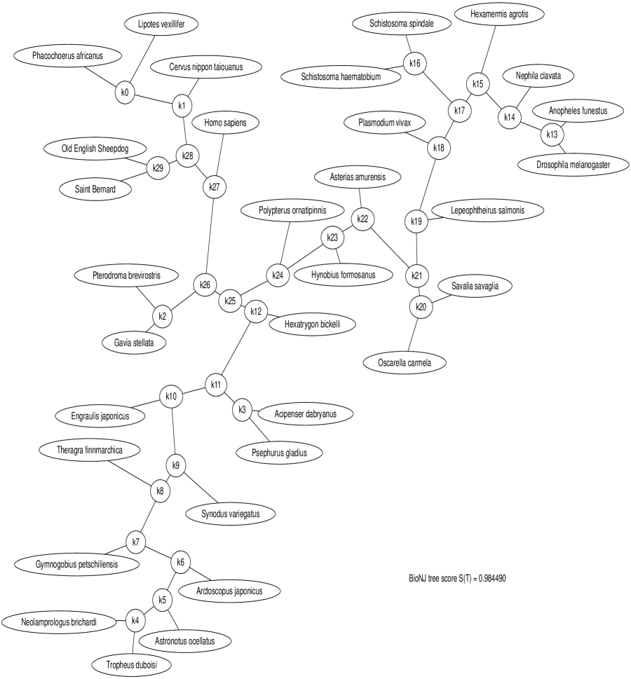
Figure 9: NJ=BioNJ tree from SplitsTree

changes in the structure of the tree. Figure 9 and Figure 10 depict one example showing both BioNJ=NJ and CompLearn trees applied to the same input matrix from one of the natural data test cases described above. In this case there are important differences in placement of at least two species; Hexatrygon bickelli and Synodus variegatus.

Figure 10: CompLearn tree for comparison with previous Figure

Although we can not know for sure the true maximum value that can be attained for the $S(T)$, given an arbitrary distance matrix, we can still define a useful quantity. Let

$$R(T)=1.0-S(T),$$ (VII.1)

and term $R(T)$ the room for improvement for tree $T$. This is especially apt in cases like the present one where we know that the optimal tree $T_{\rm opt}$ has $S(T_{\rm opt})$ close to 1. Suppose CompLearn produces tree $T$ in trial $t$ and SplitsTree produces tree $T^{\prime}$ in trial $t$. Define $R_{C}(t)=R(T)$ and $R_{S}(t)=R(T^{\prime})$ using (VII.1). We can compute the decibel gain $db(t)$ as the logarithm of the ratio of room for improvement in trial $t$ of SplitsTree’s answer versus CompLearn’s answer with the formula

$$db(t)=10\log_{10}\frac{R_{S}(T)}{R_{C}(T)}.$$ (VII.2)

Hence if $db(t)=1$ then $R_{S}(T)=10^{1/10}R_{C}(T)\approx 1.3R_{C}(T)$, and $db(t)=2$ means that $R_{S}(T)=10^{1/5}R_{C}(T)\approx 1.6R_{C}(T)$. This is statistically significant according to almost every reasonable criterion. Note that the room for improvement decibel gain $db(t)$ in (VII.2) represents also a conservative estimate of the true improvement decibel gain in real error terms. This is because the true maximum $S(T)$ score of a tree $T$ resulting from a distance matrix is always less than or equal to 1. Using the $S(T_{\rm opt})$ value of the real optimal tree $T_{\rm opt}$ instead of 1 would only make the gain more extreme. We plot the decibel room for improvement gain in Figure 11, using different binning boundaries than in Figure 8. On the horizontal axis the bins are displayed where for every trial $t$ we put $db(t)$ in the appropriate bin. On the vertical axis the percentage of the number of elements in a particular bin to the total is depicted.

Because now we use different boundaries for each bin, the percentage of trials with the same room for improvement for both CompLearn and SplitsTree is slightly higher than the percentage of trials with the same $S(T)$ values between CompLearn and SplitsTree in Figure 8. Yet now we can see the important difference in room for improvement between CompLearn and SplitsTree expressed in decibels. Thus, about 38% of the CompLearn trials gives no positive integer decibel reduction in room for improvement over the SplitsTree performance (and 1% gave a negative reduction). About 27% gives a 1db reduction in room for improvement, about 22% gives a 2db reduction in room for improvement, about 10% gives a 3db in room for improvement. Overall, about 61% of the CompLearn trials gives a 1 or more decibel reduction in room for improvement over the SplitsTree performance. In more than 1/3 of the trials CompLearn achieves at least a 2db reduction in room for improvement as compared to SplitsTree.

Figure 11: Decibel error reduction from CompLearn

VIII Conclusion

We have introduced a new quartet tree problem, the Minimum Quartet Tree Cost (MQTC) problem, suited for general hierarchical clustering. This new method relies on global optimization of the constructed tree in contrast to bottom-up or top-down methods that can get stuck in local optima, such as Quartet Puzzling, neighbor joining, and the like. Is is shown that this MQTC problem is NP-hard by a reduction to the (weighted) Maximum Quartet Consistency (MQC) problem that is more suited for the restricted case of biological phylogeny. Moreover, if there is a polynomial time approximation scheme (PTAS) for the MQTC optimization problem, then P=NP. Given the hardness of the MQTC problem we introduce a Monte Carlo heuristic based on randomized hill climbing. This heuristic runs in time which is theoretically $\Omega(n^{4})$ per generation where $n$ is the number of objects, and $O(n^{5})$ per generation in the implemented version. The improvement in Section V based on the distance matrix and quartet topology costs in (V.1) runs in time $O(n^{3})$ per generation both as algorithm and implementation. The new method including the improvement is available for general use in the open software CompLearn Toolkit [9] from version 1.1.3 onward. It has been used widely for general hierarchical clustering and also for biological phylogeny. Here, we tested our MQTC heuristic on artificial data and natural data, and compared it with the neighbor-joining method available in the (highly competitive) SplitsTree package (version 4. 6) designed for tree-structured data in Biological Phylogeny. (BioNJ and NJ in the SplitsTree package always gave the same results in our experiments, so we treat them as one, and the UPMG method in the SplitsTree package did not work for us.) To make the comparison more disadvantageous to our MQTC heuristic and more advantageous to SplitsTree we tested it on tree-structured data, rather than general hierarchical clustering on data of unknown structure. SplitsTree was generally slower (sometimes 10 seconds versus 6 seconds for CompLearn version 1.1.3 and later, that is, 2/3rd more) than our MQTC heuristic with the improvements in Section V. On our artificial data experiments both our MQTC heuristic and the SplitsTree methods gave 100% correct results. On the natural data experiments the average case of our MQTC heuristic was better than the best case of the SplitsTree heuristics. To amplify the differences we compared the decibel gain in room for improvement of SplitsTree’s answers versus our MQTC heuristic’s answers. In 61% of the trials our MQTC heuristic’s performance gave a positive integer decibel reduction in room for improvement over SplitsTree’s performance, and in 33% of the trials our MQTC heuristic’s performance gave a 2db reduction in room for improvement over SplitsTree. Other heuristics for the MQTC optimization problem are recently given in [17]. But even the best method in [17] has a slower running time for natural data (with $n=32$ typically about 50%) than the implementation of the MQTC heuristic in CompLearn from version 1.1.3 onward.

-A Sufficiency of the Set of Simple Mutations

Theorem .1

Every ternary tree with $n$ leaves labeled $l_{1},l_{2},\ldots,l_{n}$ and $n-2$ unlabeled internal nodes can be transformed in every other ternary tree with $n$ leaves labeled $l_{1},l_{2},\ldots,l_{n}$ and $n-2$ unlabeled internal nodes by a sequence of $f(n)$ mutations consisting of subtree to leaf swaps or leaf to leaf swaps where $f(3)\leq 3$ and $f(n)\leq 5n-16$ for $n\geq 4$.

Proof:

For convenience of the discussion we attach labels to the internal nodes, but actually the internal nodes are unlabeled, only the leaves are labeled.. The proof is by induction on the number of nodes.

Base case: $n=3$. There is one internal node, so the theorem is vacuously true. For $n=4$ there are two internal nodes, so the theorem is true as well using at most one leaf swap.

Induction: Assume the theorem is correct for every $k$ with $4\leq k<n$. We prove that it holds for $k=n$. For $n>4$ consider a ternary tree $T_{0}$ with $n-2$ unlabeled internal nodes $1,2,\ldots,(n-2)$ and $n$ labeled leaves that has to be transformed into a ternary tree $T_{1}$ with the same unlabeled internal nodes and labeled leaves.

Assume that the initial tree $T_{0}$ has a path $z-x-y$ where $y$ is an end internal node with two leaves and $x$ is an internal node with one leaf. If $T_{0}$ is not of that form then we make it of that form by a subtree to leaf swap: Take another end internal node $u$ (possibly $z$) and swap the 3-node tree rooted at $u$ ($u$ and its two leaves) with a leaf of $y$. This results in a path $x-y-u$ where $u$ is an end internal node with two leaves and $y$ is an internal node with a single leaf. We start from the resulting tree which we call $T_{0}$ now.

For the sake of the argument we number the nodes so that $n-2$ is an end internal node connected to an internal node $n-3$ which has a single leaf $l$. Glue the internal nodes $n-3$ and $n-2$ and the leaf $l$ together in a single internal node now denoted as $n-3$. The new $n-3$ is an end internal node connected to two leaves formerly connected to the old $n-2$. This results in an $n-3$ unlabeled internal node ternary tree $T^{\prime}_{0}$ with $n-1$ labeled leaves.

By the induction assumption we can transform $T^{\prime}_{0}$ into any ternary tree $T^{\prime}_{1}$ with $n-3$ unlabeled internal nodes and $n-1$ labeled leaves in $f(n-1)$ subtree to leaf or leaf to leaf mutations. Take $T^{\prime}_{1}$ to be a subtree of $T_{1}$ with the following exceptions. Since $T_{1}$ has one more internal node than $T_{1}^{\prime}$ we can choose that extra internal node as an end internal node attached to tree $T_{1}^{\prime}$ at the place where there is now a leaf. Let that leaf be leaf $l^{\prime}$. Note that leaf $l$ is not a leaf of $T_{1}^{\prime}$ (since it is incorporated in internal node $n-3$). If $l$ should be a leaf of $T^{\prime}_{1}$ to make it a subtree of $T_{1}$ then we swap $l$ with the leaf $l^{\prime\prime}$ in the place where $l$ has to go in a leaf-to-leaf swap. For convenience we still denote the leaf left in the composite node $n-3$ by $l$.

Now expand in $T^{\prime}_{1}$ the internal node $n-3$ into the path $(n-3)-(n-2)$ together with leaf $l$ connected to $(n-3)$. This yields a ternary tree with $n-2$ unlabeled internal nodes and $n$ labeled leaves. There are three cases.

Case 1. Initially, in $T^{\prime}_{1}$ the node $n-3$ is an end internal node connected to an internal node $u$ as in the path $u-(n-3)$. The expansion takes us to the situation that we have a path $u-(n-3)-(n-2)$ and leaf $l$ connected to $n-3$.

The old internal node $n-3$ being an end internal node had two leaves. In the path $(n-3)-(n-2)$ both these leaves stay connected to the new end internal node $n-2$ and leaf $l$ stays connected to $n-3$.

Assume first that $l^{\prime}$ is not in de 5-node subtree rooted at the new $n-3$ containing the path $(n-3)-(n-2)$. We interchange this 5-node subtree with the leaf $l^{\prime}$. Next, we interchange the 3-node subtree rooted at $n-2$ with the leaf $l^{\prime}$ at its new location. In this way, $n-3$ being now in the former position of leaf $l^{\prime}$ is the missing internal node of $T_{1}$. The new internal node $n-3$ is an end internal node with two leaves $l,l^{\prime}$ of which $l^{\prime}$ is in the correct position. There is still the leaf $l^{\prime\prime}$ being possibly in the wrong position. All the other leaves are in the correct position for $T_{1}$. After we swap the leaves $l,l^{\prime\prime}$ if necessary, all leaves are in the correct position.

Assume second that $l^{\prime}$ is in the subtree rooted at $n-3$ containing the path $(n-3)-(n-2)$. Then, the new $n-2$ being an end internal node in the former position of leaf $l^{\prime}$ is the missing internal node of $T_{1}$.

The total number of mutations used is at most three consisting of two subtree to leaf swaps and possibly one leaf to leaf swap.

Case 2. Initially, the node $n-3$ in $T_{1}^{\prime}$ is connected to two internal nodes yielding a path $u-(n-3)-v$ such that $n-3$ is connected also to one leaf, say $l^{\prime\prime\prime}$. The expansion takes us to the situation that we have a path $u-(n-3)-(n-2)-v$. The old internal node $n-3$ was connected to leaf $l^{\prime\prime\prime}$ which leaf is now connected to $n-2$. The leaf $l$ is still connected to the new $n-3$.

Assume first that $l^{\prime}$ is not in the subtree rooted at the new $n-3$ (containing $u-(n-3)$). We interchange the subtree rooted at $n-3$ (containing $u-(n-3)$) with leaf $l^{\prime}$. Next we interchange the subtree rooted at $u$ (not containing $n-3$ and leaf $l$) with $l^{\prime}$ again. Now the new $n-3$ takes the place of the missing internal node of $T_{1}$ and it is an end internal node connected to leaves $l,l^{\prime}$. Of these, leaf $l^{\prime}$ is in correct position. All the other leaves except possibly $l,l^{\prime\prime}$ are in correct position for $T_{1}$. If necessary we interchange leaves $l,l^{\prime\prime}$.

Assume second that $l^{\prime}$ is in the subtree rooted at the new $n-3$ (containing $u-(n-3)$). Interchange the subtree rooted at $n-3$ (containing $(n-3)-(n-2)$) with leaf $l^{\prime}$. Next we interchange the subtree rooted at $n-2$ (not containing $n-3$ and leaf $l$) with $l^{\prime}$ again. Now the new $n-3$ takes the place of the missing internal node of $T_{1}$ and it is an end internal node connected to leaves $l,l^{\prime}$. Of these, leaf $l^{\prime}$ is in correct position. All the other leaves except possibly $l,l^{\prime\prime}$ are in correct position for $T_{1}$. If necessary we interchange leaves $l,l^{\prime\prime}$.

The total number of mutations used is at most three consisting of two subtree to leaf swaps and possibly one leaf to leaf swap.

Case 3. Initially, in $T_{1}^{\prime}$ the node $n-3$ is connected to three internal nodes forming the path $u-(n-3)-v$ and there is a path $w-(n-3)$ with $w\neq u,v$. The expansion yields the path $u-(n-3)-(n-2)-v$ with leaf $l$ connected to $n-3$ and $n-2$ is also in a path $w-(n-2)$.

Assume first that $l^{\prime}$ is not in the subtree rooted at the new $n-3$ (containing $u-(n-3)$). We interchange the subtree rooted at the new $n-3$ containing the edge $u-(n-3)$ and leaf $l$ with the leaf $l^{\prime}$. Subsequently, we interchange the subtree rooted at $u$ (not containing $n-3$ and the connected leaf $l$) with $l^{\prime}$ again. Now node $n-3$ is in the position of the missing internal node of $T_{1}^{\prime}$ and it is an end internal node with two leaves $l,l^{\prime}$. Of these, $l^{\prime}$ is in correct position. Moreover, all the other leaves are in correct position except possibly $l,l^{\prime\prime}$. If necessary we interchange leaves $l,l^{\prime\prime}$.

Assume second that $l^{\prime}$ is in the subtree rooted at the new $n-3$ (containing $u-(n-3)$). Interchange the subtree rooted at the new $n-3$ containing the edge $(n-3)-(n-2)$ and leaf $l$ with the leaf $l^{\prime}$. Subsequently, we interchange the subtree rooted at $n-2$ (not containing $n-3$ and the connected leaf $l$) with $l^{\prime}$ again. Now node $n-3$ is in the position of the missing internal node of $T_{1}^{\prime}$ and it is an end internal node with two leaves $l,l^{\prime}$. Of these, $l^{\prime}$ is in correct position. Moreover, all the other leaves are in correct position except possibly $l,l^{\prime\prime}$. If necessary we interchange leaves $l,l^{\prime\prime}$.

The total number of mutations used is at most three consisting of two subtree to leaf swaps and possibly one leaf to leaf swap.

We count the number of mutations as follows. Initially, tree $T_{1}^{\prime}$ required at most $f(n-1)$ mutations to be obtained from tree $T_{0}^{\prime}$. By the above analysis $f(n)\leq f(n-1)+5$ (remember the possibly necessary initial subtree to leaf swap to bring $T_{0}$ in t he required form, and the possibly ncessary leaf to leaf swap between $l$ comprised in the composite node $n-3$ and $l^{\prime\prime}$ just before Case 1). The base case shows that $f(3)\leq 3$ and $f(4)\leq 4$. Hence, $f(n)\leq 4+(n-4)5=5n-16$ for $n>4$. ∎

Remark .2

Note that the only mutations used are leaf-to-leaf swaps and subtree to leaf swaps. This shows that the other mutations, that is subtree to subtree swaps, and subtree transfers are superfluous in terms of completeness. However, they may considerably reduce the number of total mutations required to go from one tree to another. Using the full set of mutations we believe it is possible to go from a ternary tree as above to another one in at most $n$ mutations as given. $\diamondsuit$

References

- [1] L. Bao, S. Bereg, Clustered SplitsNetworks, in: Combinatorial Optimization and Applications, Lect. Notes Comput. Sci., Vol. 5165, Springer, Berlin, 2008, pp. 469-478.
- [2] C.H. Bennett, P. Gács, M. Li, P.M.B. Vitányi, W. Zurek, Information Distance, IEEE Trans. Information Theory, 44:4(1998), 1407–1423.
- [3] C.H. Bennett, M. Li, B. Ma, Chain letters and evolutionary histories, Scientific American, June 2003, 76–81.
- [4] A. Ben-Dor, B. Chor, D. Graur, R. Ophir, D. Peleg, Constructing phylogenies from quartets: Elucidation of eutherian superordinal relationships, J. Computational Biology, 5:3(1998), 377–390.
- [5] V. Berry, T. Jiang, P. Kearney, M. Li, T. Wareham, Quartet cleaning: improved algorithms and simulations. Algorithms, in: Proc. 7th European Symp. (ESA99), Lect. Notes Comp. Sci., Vol. 1643, Springer, Berlin, 1999, pp. 313–324.
- [6] P. Buneman, The recovery of trees from measures of dissimilarity, in: F. Hodson, D. Kenadall, P. Tautu (Eds.), Proc. of the Anlo-Romanian conference, The Royal Society of London and the Academy of the Socialist Republic of Romania, The University Press, Edinburgh, Scotland, UK, 1971, pp. 387–395.
- [7] B. Braden, Calculating sums of infinite series, Am. Math. Monthly, 99:7(1992), 649–655.
- [8] X. Chen, B. Francia, M. Li, B. McKinnon, A. Seker, Shared information and program plagiarism detection, IEEE Trans. Information Theory, 50:7(2004), 1545–1551.
- [9] R. Cilibrasi, The CompLearn Toolkit, 2003–, http://www.complearn.org/ .
- [10] R. Cilibrasi, Statistical Inference Through Data Compression, PhD Thesis, ILLC DS-2007-01, University of Amsterdam, 2007.
- [11] R. Cilibrasi, P.M.B. Vitanyi, R. de Wolf, Algorithmic clustering of music based on string compression, Computer Music J., 28:4(2004), 49-67.
- [12] R. Cilibrasi, P.M.B. Vitanyi, Clustering by compression, IEEE Trans. Information Theory, 51:4(2005), 1523–1545.
- [13] R.L. Cilibrasi, P.M.B. Vitanyi, The Google Similarity Distance, IEEE Trans. Knowledge and Data Engineering, 19:3(2007), 370–383.
- [14] CLUSTAG: hierarchical clustering and graph methods for selecting tag SNPs, Bioinformatics, 21:8(2005), 1735–1736.
- [15] H. Colonius, H.H. Schulze, Trees constructed from empirical relations, Braunschweiger Berichte as dem Institut für Psychologie, 1(1977).
- [16] H. Colonius, H.H. Schulze, Tree structures for proximity data. British J. Math. Stat. Psych., 34(1981), 167–180.
- [17] S. Consoli, K. Darby-Dowman, G. Geleijnse, J. Korst, S. Pauws, Heuristic approaches for the quartet method of hierarchical clustering, IEEE Trans. Knowledge Data Engin., To appear.
- [18] C. Costa Santos, J. Bernardes, P.M.B. Vitanyi, L. Antunes, Clustering fetal heart rate tracings by compression, in: Proc. 19th IEEE Symp. Computer-Based Medical Systems, 2006, 685–690
- [19] R.O. Duda, P.E. Hart, D.G. Stork, Pattern Classification, second edition, Wiley Interscience, 2001.
- [20] J. Felsenstein, Evolutionary trees from DNA sequences: a maximum likelihood approach, J. Molecular Evolution, 17(1981), 368–376.
- [21] O. Gascuel, BIONJ: an improved version of the NJ algorithm based on a simple model of sequence data, Mol. Biol. Evol., 14(1997), 685–695.
- [22] D. H. Huson, D. Bryant, Application of Phylogenetic Networks in Evolutionary Studies, Mol. Biol. Evol., 23:2(2006), 254–267.
- [23] S.C. Johnson, Hierarchical clustering schemes, Psychometrika, 32:3(1967), 241–254.
- [24] T. Jiang, P. Kearney, and M. Li. A polynomial time approximation scheme for inferring evolutionary trees from quartet topologies and its application, SIAM J. Computing, 30:6(2000), 1942–1961.
- [25] P.E. Kearney, Ordinal quartet method, in: Proc. 2nd Int. Conf. Comput. Molecular Biology, 1998, 125–134.
-
[26]
M. Keijzer, New version quartet tree management
(with comments explaining the complexity
bounds) at
http://libqsearch.sourcearchive.com/documentation/1.0.8/qsearch-tree_8c-source.html - [27] E. Keogh, S. Lonardi, C.A. Rtanamahatana, Toward parameter-free data mining, in: Proc. 10th ACM SIGKDD Int. Conf. Knowledge Discovery and Data Mining, Seattle, Washington, USA, 2004, pp. 206–215.
- [28] S. Kirkpatrick, C.D. Gelatt, M.P. Vecchi, Science, 220(1983), 671–680.
- [29] T.G. Ksiazek, et.al., A Novel Coronavirus Associated with Severe Acute Respiratory Syndrome, New England J. Medicine, Published at www.nejm.org April 10, 2003 (10.1056/NEJMoa030781).
- [30] M. Li, J.H. Badger, X. Chen, S. Kwong, P. Kearney, H. Zhang, An information-based sequence distance and its application to whole mitochondrial genome phylogeny, Bioinformatics, 17:2(2001), 149–154.
- [31] M. Li, P.M.B. Vitányi. Algorithmic Complexity, in: International Encyclopedia of the Social & Behavioral Sciences, N.J. Smelser, P.B. Baltes (Eds.), Pergamon, Oxford, 2001/2002, pp. 376–382.
- [32] M. Li, X. Chen, X. Li, B. Ma, P.M.B. Vitányi, The similarity metric, IEEE Trans. Information Theory, 50:12(2004), 3250–3264.
- [33] M. Li, P.M.B. Vitányi. An Introduction to Kolmogorov Complexity and its Applications, Springer, New York, third ed., 2008.
- [34] T. Liu, J. Tang, B.M.E. Moret, Quartet methods for phylogeny reconstruction from gene orders. Dept. CS and Engin., Univ. South-Carolina, Columbia, SC, USA. Manuscript 2005.
- [35] N. Metropolis, A.W. Rosenbluth, M.N. Rosenbluth, A.H. Teller, E. Teller, J. Chem. Phys., 21(1953), 1087-1092.
- [36] R. Piaggio-Talice, J. Gordon Burleigh, O. Eulenstein, Quartet supertrees. Chapter 4 in: O.R.P. Beninda-Edmonds (Ed.), Phylogenetic Supertrees: Combining Information to Reveal the Tree of Life, Computational Biology, Vol. 3 (A. Dress, series Ed.), Kluwer Academic Publishers, 2004, pp. 173–191.
- [37] U. Roshan, B.M.E. Moret, T. Warnow, T.L. Williams, Performance of supertree methods on various datasets decompositions, in: O.R.P. Beninda-Edmonds (Ed.), Phylogenetic Supertrees: Combining Information to Reveal the Tree of Life, Computational Biology, Vol. 3 (A. Dress, series Ed.), Kluwer Academic Publishers, 2004, pp. 301–328.
- [38] N. Saitou, M. Nei, The neighbor-joining method: a new method for reconstructing phylogenetic trees, Mol. Biol. Evol., 4(1987), 406–425.
- [39] S. Snir, T. Warnow, S. Rao, Short Quartet Puzzling: A new quartet-based phylogeny reconstruction algorithm, J. Comput. Biol., 15:1(2008), 91–103.
- [40] M. Steel, The complexity of reconstructing trees form qualitative characters and subtrees, J. Classification, 9(1992), 91–116.
- [41] K. Strimmer, A. von Haeseler, Quartet Puzzling: A quartet maximum-likelihood method for reconstructing tree topologies, Mol. Biol. Evol., 13:7(1996), 964–969.
- [42] P.M.B. Vitanyi, A discipline of evolutionary programming, Theor. Comp. Sci., 241:1-2(2000), 3–23.
- [43] S. Wehner, Analyzing worms and network traffic using compression, J. Comput. Security, 15(2007), 303–320.
- [44] J. Weyer-Menkoff, C. Devauchelle, A. Grossmann, S. Grünewald, Integer linear programming as a tool for constructing trees from quartet data, Comput Biol Chem., 29:3(2005), 196-203.