Two-dimensional Bose-Einstein condensate under pressure

Abstract

Evading the Mermin-Wagner-Hohenberg no-go theorem and revisiting with rigor the ideal Bose gas confined in a square box, we explore a discrete phase transition in two spatial dimensions. Through both analytic and numerical methods we verify that thermodynamic instability emerges if the number of particles is sufficiently yet finitely large: specifically $N\geq 35131$. The instability implies that the isobar of the gas zigzags on the temperature-volume plane, featuring supercooling and superheating phenomena. The Bose-Einstein condensation then can persist from absolute zero to the superheating temperature. Without necessarily taking the large $N$ limit, under constant pressure condition, the condensation takes place discretely both in the momentum and in the position spaces. Our result is applicable to a harmonic trap. We assert that experimentally observed Bose-Einstein condensations of harmonically trapped atomic gases are a first-order phase transition which involves a discrete change of the density at the center of the trap.

Keywords: ideal Bose gas, emergence, first-order phase transition, two dimensions.

1 Introduction

The existence of Bose-Einstein condensate (BEC) in two spatial dimensions ($2D$) is a subtle issue, attracting a wide range of interests from both theoretical and experimental perspectives. The Mermin-Wagner-Hohenberg (MWH) theorem [1, 2] prohibits free bosons from condensing on a homogeneous infinite plane via long-range thermal fluctuations. The Berezinskii-Kosterlitz-Thouless (BKT) mechanism then provides an alternative explanation of a quasi-transition to superfluid without condensation [3, 4]. On the other hand, $2D$ BEC has been realized in experiments for harmonically trapped atomic gases, c.f. [5] and references therein, in support of some analytic estimations [6, 7, 8].

One related deep question is whether a finite system can feature a mathematical singularity or not. While Anderson once stated “More is different” [9], the question we are addressing is “How many is different?” [10]. Constrained by the analyticity of the partition function [11] one may argue that “More is the same: infinitely more is different” [12]. This has motivated, especially for $3D$, the widely adopted rather axiomatic approach to discrete phase transitions where the first-order phase transition is ‘defined’ only in the thermodynamic limit. In two and one dimensions, the MWH theorem then seems to imply that Infinity is not enough: interaction is required. However, it is also true that infinity is hardly realistic and exists only in theory.

Historically, London already noted in 1954 [13] that in order to decide the question of the order of the transition one should not prescribe the volume, $V$; one has rather to use pressure, $P$, and temperature, $T$ as independent variables. The specific heats per particle at constant volume, $c_{V}$, and constant pressure, $c_{P}$, can be quite different for a finite system from the theoretical consideration of statistical physics. Being an analytic function, $c_{V}$ should be finite for a finite system. On the other hand, $c_{P}$ is generically given by a fraction of two analytic functions and when the denominator vanishes, namely on the spinodal curve [14, 15, 16], it becomes singular, for further discussions see e.g. [17, 18] as well as Eq.(6) of [19].

Essentially, one can easily boil water if one keeps not the volume (or density) but the pressure constant [19, 10]. Indeed, involving two of the authors, it has been shown recently that the $c_{P}$ of $3D$ ideal Bose gases can diverge even for a finite number of particles [19, 20, 21]. This is only possible because thermodynamic instability emerges making the isobar zigzag on the $(T,V)$-plane when the number of particles is greater than or equal to a definite value. Such critical number depends on the shape of the box but not the size, thanks to the existing scale symmetry of the ideal gas: for example the critical number is precisely $7616$ for the $3D$ cubic box [19]. This might appear mathematically unnatural and random, but can be a physical answer to the question, How many is different?. Because the isobar zigzags on the $(T,V)$-plane, when the temperature increases under constant pressure, the volume and hence the density must make a ‘discrete’ jump. Since all the physical quantities are functions of temperature and density, the discrete jump then implies or realizes a first-order phase transition.

In this work, we turn our attention to a $2D$ ideal Bose gas which is confined in a square box. In contrast to the homogeneous infinite plane for which the MWH no-go theorem surely holds, the presence of the box breaks the translational symmetry and converts the energy spectrum from continuous uncountable infinite to discrete countable infinite. This leads to fundamental differences between the two systems, effectively classical v.s. quantum, which should persist even in the large $V$ limit of the box. As the harmonic potential allows $2D$ BEC to occur, it is physically natural to expect that a “small” box should do so as well.

In fact, it has been known from 1970s that $2D$ BEC may occur under the constant pressure condition [17, 18]. The critical temperature was first obtained by Imry et al. in [17] and its leading order finite-size correction was analyzed by Chaba and Patria in [18]. In particular, by insisting the thermodynamic stability, the latter two authors found a pair of nearby critical temperatures. Yet, as they remarked in their section III, the physical interpretation was somewhat “awkward” and “more refined treatment of the problem” was desirable.

It is the purpose of the present paper to provide such a desired complementary analysis, helped by modern computing power. Treating the exact mathematical expressions numerically –which all descend from a single partition function– we show that thermodynamic instability, satisfying the spinodal condition, emerges if the number of particles is sufficiently yet finitely large. Specifically for the $2D$ ideal Bose gas confined in a square box, we demonstrate that the isobar zigzags on the temperature-volume plane if $N\geq N_{c}=35131$. Consequently, the $2D$ BEC becomes a first-order phase transition under constant pressure, similar to the $3D$ ideal Bose gases [19, 20, 21]. We identify the two critical points found in [18] as the supercooling and the superheating spinodal points which correspond to the two turning points of the zigzagging isobar. Between the supercooling and the superheating temperatures the volume is triple-valued including one unstable configuration. We also improve the analytic approximation of [18] by newly obtaining ‘double logarithmic’ sub-leading corrections.

Our main results are spelled in Eqs.(15,16) and depicted in Figures 2, 3, 4, which are methodologically twofold: i) analytical for large $N$ and ii) numerical for arbitrary $N$. They are in excellent agreement, for which the double logarithmic terms are necessary. While much of the present $2D$ results are parallel to the $3D$ cases [19, 20, 21], there are also some differences. Lastly, we comment on the implication of our results to the experimentally observed BEC of harmonically trapped atomic gases.

2 Setup

We consider the textbook $2D$ system of an ideal Bose gas which is confined in a square box, with the area (or $2D$ volume), $V$, and the number of particles, $N$. Experimental realization of such a system has just begun this year [22]. In a parallel manner to Ref.[21] (c.f. [23]), here we focus on the grand canonical ensemble with the fixed average number of particles. From the non-relativistic dispersion relation, $E={\vec{p}{}^{\,2}}/{(2m)}$, the grand canonical partition function is actually a two-variable function depending on the fugacity, $z$, and the combination of the temperature and the area, $TV$. This implies a scaling symmetry: different sizes of the volume can be traded with different scales of the temperature. In particular, the small volume or the ‘confining’ potential effect should persist for large volume.

Specifically we set, as for the two dimensionless fundamental variables in our analysis,

$$\begin{array}[]{ll}\varepsilon:=\frac{\pi^{2}\hbar^{2}}{2mk_{{\scriptscriptstyle{\rm B}}}TV}\,,{}{}&~{}~{}\sigma:=-\ln z\,.\end{array}$$ (1)

In terms of these, the grand canonical partition function reads

$$\ln{\cal Z}(\varepsilon,\sigma)=-{\sum}_{\vec{n}\in{\mathbb{N}}^{2}}\,\ln\!\left(1-e^{-\varepsilon\vec{n}^{2}-\sigma}\right)\,.$$ (2)

With the Dirichlet boundary condition which we deliberately impose, $\vec{n}=(n_{1},n_{2})\in{\mathbb{N}}^{2}$ is a positive integer-valued $2D$ lattice vector, such that the lowest value of $\vec{n}^{2}$ is two and $\sigma$ is bounded from below as $\sigma>-2\varepsilon$.

The average number of particles is then

$$N(\varepsilon,\sigma)=-\partial_{\sigma}\ln{\cal Z}(\varepsilon,\sigma)\,,$$ (3)

and the standard expression, $P=k_{{\scriptscriptstyle{\rm B}}}T\partial_{V}\ln{\cal Z}(T,V,z)$, of the pressure is equivalent to

$${{\cal T}}_{{\scriptscriptstyle{P}}}(\varepsilon,\sigma):=\!\left(\frac{2m}{\pi^{2}\hbar^{2}P}\right)^{\frac{1}{2}}\!k_{{\scriptscriptstyle{\rm B}}}T=\left[-\varepsilon^{2}\partial_{\varepsilon}\ln{\cal Z}(\varepsilon,\sigma)\right]^{-\frac{1}{2}}.$$ (4)

Being a combination of  $T$ and $P$, this dimensionless quantity, ${{\cal T}}_{{\scriptscriptstyle{P}}}$, can denote the physical temperature on an arbitrarily given isobar. Similarly we may define a dimensionless “volume”,

$${{\cal V}}_{{\scriptscriptstyle{P}}}(\varepsilon,\sigma):=\left(\frac{2m}{\pi^{2}\hbar^{2}}P\right)^{\frac{1}{2}}V=\left[-\partial_{\varepsilon}\ln{\cal Z}(\varepsilon,\sigma)\right]^{\frac{1}{2}}\,,$$ (5)

and another dimensionless “temperature”,

$${{{\cal T}}_{{\rho}}(\varepsilon,\sigma):=\frac{2mk_{{\scriptscriptstyle{\rm B}}}TV}{\pi^{2}\hbar^{2}N}=\left[-\varepsilon\partial_{\sigma}\ln{\cal Z}(\varepsilon,\sigma)\right]^{-1}\,.}$$ (6)

Further, the number of particles on the ground state is

$${N_{0}(\varepsilon,\sigma)=\partial_{\sigma}\ln\!\left(1-e^{-2\varepsilon-\sigma}\right)=\left(e^{2\varepsilon+\sigma}-1\right)^{-1}\,.}$$ (7)

As we already denoted, $N$, $N_{0}$, ${{\cal T}}_{{\scriptscriptstyle{P}}}$, ${{\cal V}}_{{\scriptscriptstyle{P}}}$ and ${{\cal T}}_{{\rho}}$ are all functions of the two variables, $\varepsilon$, $\sigma$ only. They satisfy identities,

$$\begin{array}[]{ll}{{\cal T}}_{{\scriptscriptstyle{P}}}(\varepsilon,\sigma){{\cal V}}_{{\scriptscriptstyle{P}}}(\varepsilon,\sigma)=\varepsilon^{-1}\,,&\quad{{\cal T}}_{{\rho}}(\varepsilon,\sigma)N(\varepsilon,\sigma)=\varepsilon^{-1}\,.\end{array}$$ (8)

Generically, the superheating (BEC) and the supercooling points correspond to the two turning points of an isobar which zigzags on the $(T,V)$-plane, satisfying the spinodal curve condition, ${{\rm d}N}=0$, ${{\rm d}P}=0$, ${{\rm d}T}=0$ [15, 14, 16, 20, 21]. In our case, the spinodal curve is to be positioned on the $(\varepsilon,\sigma)$-plane (c.f. Figure 1) to satisfy

$$\begin{array}[]{ll}{{\rm d}N(\varepsilon,\sigma)=0}\,,&\quad{{\rm d}{{\cal T}}_{{\scriptscriptstyle{P}}}(\varepsilon,\sigma)=0}\,,\end{array}$$ (9)

and hence the following linear equation must admit a nontrivial solution,

$$\left(\begin{array}[]{c}0\\ 0\end{array}\right)=\left(\begin{array}[]{cc}\partial_{\varepsilon}\partial_{\sigma}\ln{\cal Z}&\partial_{\sigma}^{2}\ln{\cal Z}\\ \left(2\varepsilon^{-1}\partial_{\varepsilon}+\partial_{\varepsilon}^{2}\right)\ln{\cal Z{}}&\partial_{\varepsilon}\partial_{\sigma}\ln{\cal Z}\end{array}\right)\left(\begin{array}[]{c}{\rm d}\varepsilon\\ {\rm d}\sigma\end{array}\right)\,.$$ (10)

Consequently the ${2\times 2}$ matrix must be singular,

$$\Phi:=\det\left(\begin{array}[]{cc}\partial_{\varepsilon}\partial_{\sigma}\ln{\cal Z}&\partial_{\sigma}^{2}\ln{\cal Z}\\ \left(2\varepsilon^{-1}\partial_{\varepsilon}+\partial_{\varepsilon}^{2}\right)\ln{\cal Z{}}&\partial_{\varepsilon}\partial_{\sigma}\ln{\cal Z}\end{array}\right)\equiv 0\,.$$ (11)

This algebraic equation determines the spinodal curve on the $(\varepsilon,\sigma)$-plane. For consistency, we note that the determinant, $\Phi$, is proportional to $\left.\frac{{\rm d}{{\cal T}}_{{\scriptscriptstyle{P}}}}{{\rm d}{{\cal V}}_{{\scriptscriptstyle{P}}}}\right|_{N}$, as

$${\left.\frac{{\rm d}\ln{{\cal T}}_{{\scriptscriptstyle{P}}}}{{\rm d}\ln{{\cal V}}_{{\scriptscriptstyle{P}}}}\right|_{N}=\frac{\Phi}{\,\left(\partial_{\varepsilon}^{2}\ln{\cal Z}\right)\left(\partial_{\sigma}^{2}\ln{\cal Z}\right)-\left(\partial_{\varepsilon}\partial_{\sigma}\ln{\cal Z}\right)^{2}}\,,}$$ (12)

where the denominator on the right hand side can be shown to be positive definite [21]. Hence, the vanishing of the determinant is, as expected, equivalent to the vanishing of $\left.\frac{{\rm d}{{\cal T}}_{{\scriptscriptstyle{P}}}}{{\rm d}{{\cal V}}_{{\scriptscriptstyle{P}}}}\right|_{N}$, implying a zigzagging isobar (see Figure 3).

Our aims are first to solve (11), second to express the solutions in terms of the more physical variables, $N$, ${{\cal T}}_{{\scriptscriptstyle{P}}}$, ${{\cal V}}_{{\scriptscriptstyle{P}}}$, ${{\cal T}}_{{\rho}}$ using (3), (4), (5), (6), and finally to confirm BEC, i.e. $N_{0}/N\rightarrow 1$, at the superheating point. Searching for spinodal curves approaching the large $N$ limit, we shall focus on the region, $\varepsilon\rightarrow 0^{+}$ and $\sigma+2\varepsilon\rightarrow 0^{+}$.

A contains our technical yet self-contained derivation of the solutions which we spell below.

3 Main Results

Our solutions of the spinodal curves solving the constraint (11) on the $(\varepsilon,\sigma)$-plane are are depicted in Figure 1. Especially near to the region, $\varepsilon\rightarrow 0^{+}$, $\sigma+2\varepsilon\rightarrow 0^{+}$ (as for large $N$), we obtain the following analytic approximate solutions.

• $\ast$ Supercooling spinodal curve of $h=\frac{1}{2}$,

  $$\begin{array}[]{cll}\sigma&\simeq&-2\varepsilon+{\frac{2\zeta(\frac{3}{2})}{\sqrt{\pi}}\left(\ln\varepsilon-4\ln|\ln\varepsilon|\right)^{-2}\varepsilon^{\frac{1}{2}}\,,}\\ \varepsilon&\simeq&{\frac{\pi}{8}}N^{-1}\left(\ln N+3\ln\ln N\right)\,.\end{array}$$ (13)

• ${\ast\ast}$ Superheating (BEC) spinodal curve of $h=\frac{3}{2}$,

  $$\begin{array}[]{ll}\sigma\simeq-2\varepsilon+{\frac{32}{\sqrt{\pi}\zeta(\frac{3}{2})}\varepsilon^{\frac{3}{2}}\,,}&\quad\varepsilon\simeq{\left[\frac{1}{32}\sqrt{\pi}\zeta(\frac{3}{2})\right]^{\frac{2}{3}}N^{-\frac{2}{3}}\,.}\end{array}$$ (14)

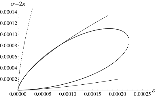
Figure 1: The supercooling and the superheating spinodal curves on the $(\sigma+2\varepsilon,\varepsilon)$-plane. The dotted closed curve is from the numerical computations based on the exact formula (11). The upper and lower solid lines correspond to our analytic approximate solutions, (13) and (14) respectively. The dashed line denotes a less-accurate supercooling approximation [18] without the double logarithmic term in (13). The interior of the dotted closed curve is thermodynamically unstable.

The above analytic approximation agrees with the results obtained by Chaba and Pathria [18], where the double logarithmic terms were yet neglected. As shown in Figures 1, 2, the terms appear crucial to match with the numerical computations. Besides the double logarithmic corrections, another novel contribution of this work is to identify the two spinodal curves as the supercooling and the superheating turning points of the zigzagging isobar on $(T,V)$-plane, see Figures 3, 4.

In terms of the physical variables, $N$, ${{\cal T}}_{{\scriptscriptstyle{P}}}$ (4), ${{\cal V}}_{{\scriptscriptstyle{P}}}$ (5), ${{\cal T}}_{{\rho}}$ (6), the supercooling and the superheating (BEC) points are as follows, c.f. [18].

• $\ast$ Supercooling point :

  $$\begin{array}[]{l}{{\cal T}}_{{\scriptscriptstyle{P}}}^{\ast}/{{{\cal T}}_{{\scriptscriptstyle{P}}}^{{\rm\scriptscriptstyle{BEC}}}}\simeq 1+{\frac{3\sqrt{2}}{4\pi^{2}}\zeta(\frac{3}{2})}\left(\frac{\ln N+3\ln\ln N}{N}\right)^{\frac{1}{2}}\,,\\ {{\cal V}}_{{\scriptscriptstyle{P}}}^{\ast}\simeq{\sqrt{\frac{8\pi}{3}}}\frac{N}{\,\ln N+3\ln\ln N\,}\,,\\ {{\cal T}}_{{\rho}}^{\ast}\simeq\frac{8}{\pi}\left(\ln N+3\ln\ln N\right)^{-1}\,,\\ N_{0}/N\simeq{\frac{\sqrt{2}}{\zeta(\frac{3}{2})}}N^{-\frac{1}{2}}(\ln N+3\ln\ln N)^{\frac{3}{2}}\,.\end{array}$$ (15)

• ${\ast\ast}$ Superheating (BEC) point :

  $$\begin{array}[]{l}{{\cal T}}_{{\scriptscriptstyle{P}}}^{{\ast\ast}}/{{{\cal T}}_{{\scriptscriptstyle{P}}}^{{\rm\scriptscriptstyle{BEC}}}}\simeq 1+{\frac{9}{16}\left[\frac{2\zeta^{4}(\frac{3}{2})}{\pi^{7}}\right]^{\frac{1}{3}}}N^{-\frac{1}{3}}\,,\\ {{\cal V}}_{{\scriptscriptstyle{P}}}^{{\ast\ast}}\simeq{\frac{\,\pi^{\frac{7}{6}}}{\sqrt{24}}\left[\frac{32}{\zeta(\frac{3}{2})}\right]^{\frac{2}{3}}}N^{\frac{2}{3}}\,,\\ {{\cal T}}_{{\rho}}^{{\ast\ast}}\simeq\left[\frac{1}{32}\sqrt{\pi}\zeta(\frac{3}{2})\right]^{-\frac{2}{3}}N^{-\frac{1}{3}}\,,\\ N_{0}/N\simeq 1-{\left[\frac{128\pi^{2}}{27\zeta^{2}(\frac{3}{2})}\right]^{\frac{1}{3}}}N^{-\frac{1}{3}}\ln N\,.\end{array}$$ (16)

Here ${{{\cal T}}_{{\scriptscriptstyle{P}}}^{{\rm\scriptscriptstyle{BEC}}}={\sqrt{{24}/{\pi^{3}}}}}$ denotes a dimensionless constant which gives the $2D$ BEC critical temperature in the large $N$ limit [17] :

$${k_{{\scriptscriptstyle{\rm B}}}T^{{\rm\scriptscriptstyle{BEC}}}=\hbar\sqrt{\frac{12}{\pi m}P\,}\,.}$$ (17)

As we show shortly, this formula holds universally even for the $2D$ harmonic potential.

The above results lead to the phase diagram of the $2D$ ideal Bose gas on the $(T,P)$-plane: under arbitrarily fixed pressure, $P$, the state is condensate if

$${T<T^{\ast}=\frac{\hbar}{k_{{\scriptscriptstyle{\rm B}}}}\sqrt{\frac{12}{\pi m}P\,}\left[1+{\frac{3\sqrt{2}}{4\pi^{2}}\zeta(\textstyle{\frac{3}{2}})}\sqrt{\frac{\ln N+3\ln\ln N}{N}}\,\right]\,,}$$ (18)

and becomes gas if

$${T\geq T^{{\ast\ast}}=\frac{\hbar}{k_{{\scriptscriptstyle{\rm B}}}}\sqrt{\frac{12}{\pi m}P\,}\left[1+{\frac{9}{16}\sqrt[3]{\frac{2\zeta^{4}(\frac{3}{2})}{\pi^{7}N}}}\,\right]\,.}$$ (19)

Note that $T^{{\ast\ast}}>T^{\ast}$. Between the two temperatures, three states may coexist, including one unstable. In the large $N$ limit, the gap, $T^{{\ast\ast}}-T^{\ast}={\cal O}(N^{-1/3})$, becomes negligible and the two spinodal curves converge to a single line on the $(T,P)$-plane. Further the density of the superheated BEC is as high as ${N/{{\cal V}}_{{\scriptscriptstyle{P}}}^{{\ast\ast}}}={\cal O}(N^{1/3})$ and diverges in the large $N$ limit.

In contrast to the $3D$ ideal Bose gas [19, 21], the volume per particle at the supercooling point is not constant but depends inversely on $\ln N$ i.e. ${{\cal V}}_{{\scriptscriptstyle{P}}}^{\ast}/N={\cal O}(\frac{1}{\ln N})$. Hence both ${{\cal V}}_{{\scriptscriptstyle{P}}}^{\ast}/N$ and ${{\cal V}}_{{\scriptscriptstyle{P}}}^{{\ast\ast}}/N$ vanish in the large $N$ limit and therefore, once drawn on the $({{\cal T}}_{{\scriptscriptstyle{P}}},{{\cal V}}_{{\scriptscriptstyle{P}}}/N)$-plane the superheating and the supercooling points converge to the single point, $({{\cal T}}_{{\scriptscriptstyle{P}}}^{{\rm\scriptscriptstyle{BEC}}},0)$. In order to see their separation even in the large $N$ limit, it is necessary to consider a rather unusual variable, $N/(V\ln N)$, instead of the density, $N/V$. Otherwise the conventional thermodynamic limit with fixed density fails to capture the fine structure of the large $N$ behaviors of the ideal gas.

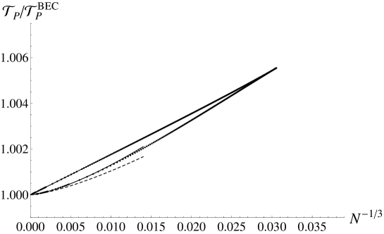
Figure 2: The supercooling (lower) and the superheating (upper) spinodal curves on the $(N^{-1/3},{{{\cal T}}_{{\scriptscriptstyle{P}}}/{{\cal T}}_{{\scriptscriptstyle{P}}}^{{\rm\scriptscriptstyle{BEC}}}})$-plane. The dotted curves are from the numerical computations based on the exact formulas, (3), (4), (11). The solid lines correspond to our analytic approximate solutions, (15), (16) for large $N$. The dashed line denotes the less-accurate analytic approximation for the supercooling curve without the double logarithmic correction, i.e. ‘$\ln\ln N$’, in (15), c.f. [18]. A pair of spinodal curves emerge at $N_{\rm{c}}\simeq 35130.3$ ($N^{-1/3}_{\rm{c}}\simeq 0.0305332$) and start to converge from $N_{\mathrm{{\scriptscriptstyle{MAX}}}}\simeq 1.43056\times 10^{6}$ ($N_{\mathrm{{\scriptscriptstyle{MAX}}}}^{-1/3}\simeq 0.00887491$) toward the large $N$ limit.

Figure 3: $2D$ BEC in the position space: if $35131\leq N<\infty$, the isobar zigzags on the $({{\cal T}}_{{\scriptscriptstyle{P}}}/{{\cal T}}_{{\scriptscriptstyle{P}}}^{{\rm\scriptscriptstyle{BEC}}},{{{\cal V}}_{{\scriptscriptstyle{P}}}/N})$-plane with the two turning points, supercooling $\ast$ (15) and superheating ${\ast\ast}$ (16).

Figure 4: $2D$ BEC in the momentum space: the number of the particles on the ground state zigzags when $35131\leq N<\infty$.

4 Consistency with a $2D$ harmonic trap

For an arbitrary gas subject to a $2D$ harmonic potential, $V(r)={{\textstyle\frac{1}{2}}}m\omega^{2}r^{2}$, let us define $N(r)$ to be the number of particles within the radius $r$ and $P(r)$ to be the radially varying pressure. They assume boundary values, ${N(0)=0}$, ${N(\infty)=N}$, $P(\infty)=0$, and satisfy the Newtonian equilibrium condition, balancing the pressure gradient and the harmonic force,

$$2\pi rP^{\prime}(r)=-mN^{\prime}(r)\omega^{2}r\,.$$ (20)

It follows then

$${P(r)=\frac{m\omega^{2}}{2\pi}\left[N-N(r)\right]\,.}$$ (21)

In particular, at the center, $r=0$, where BEC is typically observed in experiment, we have

$$P(0)=\frac{m\omega^{2}}{2\pi}N\,.$$ (22)

Substituting this into Eq.(17), we recover precisely – and satisfactorily – the known BEC critical temperature for the $2D$ harmonic trap [5, 7, 8],

$${k_{{\scriptscriptstyle{\rm B}}}T^{{\rm\scriptscriptstyle{BEC}}}=\frac{\hbar\omega}{\pi}\sqrt{6N\,}\,.}$$ (23)

It is worth while to note that the value of the central pressure (22) is true not only for the ideal gas but also for real gases, regardless of temperature, species and interactions. The derivation above is independent of them. Thus, at the center of the harmonic potential the pressure is kept fixed and the Bose-Einstein condensation can take place discretely.  

5 Discussion

To summarize, when $N\geq N_{c}=35131$, the ideal Bose gas confined in a $2D$ box reveals thermodynamic instability or a pair of spinodal curves, supercooling and superheating (BEC). Evading the MWH no-go theorem, the gas condenses discretely at finite temperature under constant pressure in both the momentum and the position spaces. As in $3D$ [19, 20, 21], this is an emergent phenomenon which finitely many bosonic identical particles can feature, without assuming the large $N$ limit.

The ideal gas represents the leading order behavior of any (weakly) interacting real gases. It is natural to expect that small interactions should deform the shape of the spinodal curve depicted in Figure 2 but hard to imagine that such interactions will make the spinodal curve completely disappear. Thus, our result should provide a novel theoretical foundation for a two-dimensional discrete phase transition of real gases.

Some reasons how our result evades the MWH theorem are as follows. Firstly, the theorem assumes the density to be finite. Yet, the density of the superheated BEC we have obtained diverges in the large $N$ limit. Therefore, the theorem is inapplicable to our case, see also [7] for related discussion. Secondly, the theorem concerns the infrared divergence of the momentum integral, $\int{\rm d}^{s}k\,\frac{1}{\,k^{2}\,}$, which diverges in one and two spatial dimensions, i.e. $s=1,2$, (see the discussion around Eqs.(18,19) in [2]). However, at the quantum level, the discrete quantum states should convert the integral to a sum over the countable states. The sum is finite and hence the theorem can be circumvented. Repulsive interactions may well prevent density from diverging as expected from real gases. As discussed above, only if the interaction does not alter the existence of the spinodal curve, a discrete phase transition should persist. Then, the second reason should survive to explain why the MWH theorem may not hold for a real quantum system of discrete spectrum.

Although a two-dimensional square box potential has been realized in a recent experiment [22], it should be hard to impose the constant pressure condition especially on small box systems. On the other hand, we have shown that the pressure at the center of the harmonic potential remains fixed for both the ideal and real gases, (22). Our result then seems to indicate that experimentally observed Bose-Einstein condensations of harmonically trapped atomic gases are a first-order phase transition which involves a discrete change of the density at least at the center of the trap, provided there are sufficiently many particles.

In this work we have focused on the grand canonical ensemble. Analyzing instead the canonical ensemble will require more computational power and most likely suggest a different value of the critical number: for example in $3D$, $N_{c}=7616$ (canonical) [19] or $N_{c}=14393$ (grand canonical) [21]. Yet, in our opinion, what matters is the existence of such a definite number, alternative to infinity, which may answer to the question, How many is different? [10]. For larger values of $N$ the differences due to different choices of the ensembles are expected to be anyhow negligible. In $3D$, the canonical ensemble results agree with those of the grand canonical ensemble within $0.1\%$ error when $N=10^{5}$ or $10^{6}$, c.f. the TABLE I in Ref.[21].

As computable from our analytic solutions, (15), (16), the gap between the supercooling and the superheating temperatures, ${{\cal T}}_{{\scriptscriptstyle{P}}}^{{\ast\ast}}-{{\cal T}}_{{\scriptscriptstyle{P}}}^{\ast}$, becomes maximal when the number of particles is equal to $N_{\mathrm{{\scriptscriptstyle{MAX}}}}\simeq 1.43056\times 10^{6}$. This also agrees with the numerical result shown in Figure 2. In a way, the two numbers, $N_{c}$ and $N_{\mathrm{{\scriptscriptstyle{MAX}}}}$, enable us to divide the Bose gas system into three quantum realms:

1. microscopic  for  ${1\leq N<N_{c}}$,

2. mesoscopic  for  ${N_{c}\leq N\leq N_{\mathrm{{\scriptscriptstyle{MAX}}}}}$,

3. macroscopic  for  ${N_{\mathrm{{\scriptscriptstyle{MAX}}}}<N\leq\infty}$.

Lastly, when $N=N_{c}$ the volume expansion ratio,

$${{{\cal V}}_{{\scriptscriptstyle{P}}}^{\ast}/{{\cal V}}_{{\scriptscriptstyle{P}}}^{{\ast\ast}}\simeq\left[\frac{\zeta(\frac{3}{2})}{\sqrt{2}\pi}\right]^{\frac{2}{3}}\!\frac{N^{\frac{1}{3}}}{\ln N+3\ln\ln N}\simeq 0.701855\times\!\frac{N^{\frac{1}{3}}}{\ln N+3\ln\ln N}\,,}$$ (24)

becomes $1.31267$ which is ‘for consistency’ of order unity.

Appendix A Analytic Approximation

To solve the spinodal condition (11) and to compute the number of particles (3), we henceforth focus on

$$\begin{array}[]{l}\partial_{\sigma}\ln{\cal Z}=\sum_{\vec{n}\in{\mathbb{N}}^{2}}\,\frac{1}{1-e^{\varepsilon\vec{n}^{2}+\sigma}}\,,\\ \varepsilon^{-1}\partial_{\varepsilon}\ln{\cal Z}=\sum_{\vec{n}\in{\mathbb{N}}^{2}}\,\frac{\varepsilon^{-1}\vec{n}^{2}}{1-e^{\varepsilon\vec{n}^{2}+\sigma}}\,,\\ \partial^{2}_{\sigma}\ln{\cal Z}=\sum_{\vec{n}\in{\mathbb{N}}^{2}}\,\frac{1}{4}\sinh^{-2}\left(\frac{\varepsilon\vec{n}^{2}+\sigma}{2}\right)\,,\\ \partial_{\varepsilon}\partial_{\sigma}\ln{\cal Z}=\sum_{\vec{n}\in{\mathbb{N}}^{2}}\,\frac{1}{4}\vec{n}^{2}\sinh^{-2}\left(\frac{\varepsilon\vec{n}^{2}+\sigma}{2}\right)\,,\\ \partial^{2}_{\varepsilon}\ln{\cal Z}=\sum_{\vec{n}\in{\mathbb{N}}^{2}}\,\frac{1}{4}(\vec{n}^{2})^{2}\sinh^{-2}\left(\frac{\varepsilon\vec{n}^{2}+\sigma}{2}\right)\,.\end{array}$$ (25)

Our computational scheme to obtain the analytic solution of (11) is, based on Ref.[21], as follows.

1. Separate the lattice sum into two parts introducing an arbitrary cutoff, $\Lambda=5,8,10,13,17,\cdots$ $(\Lambda>2)$,

   $${\sum_{\vec{n}\in{\mathbb{N}}^{2}}f(\varepsilon\vec{n}^{2})=\sum_{\vec{n}^{2}<\Lambda}f(\varepsilon\vec{n}^{2})+\sum_{\vec{n}^{2}\geq\Lambda}f(\varepsilon\vec{n}^{2})\,.}$$ (26)

2. Approximate the last sum by an integral,

   $${\quad{{\sum_{\vec{n}^{2}\geq\Lambda}}}f(\varepsilon\vec{n}^{2})\simeq{{\int_{\Lambda\varepsilon}^{\infty}}{\,{\rm d}x\,}}\left[{\frac{\pi}{4}\varepsilon^{-1}-{\frac{1}{2}}(\varepsilon x)^{-\frac{1}{2}}}\right]f(x)\,.}$$ (27)

   This formula follows from an identity,

   $${\sum_{\vec{n}\in{\mathbb{N}}^{2},\vec{n}^{2}\geq\Lambda}=\frac{1}{4}\sum_{\vec{n}\in{\mathbb{Z}}^{2},\vec{n}^{2}\geq\Lambda}-\frac{1}{2}\sum_{n\in{\mathbb{Z}},n^{2}\geq\Lambda}\,,}$$

   and the integral approximation of the right hand side [24].

3. Assume an ansatz with two positive quantities:

   $$\begin{array}[]{lll}\sigma\simeq-2\varepsilon+g\varepsilon^{h}\,,{}&~{}g>0\,,{}&~{}h>0\,.\end{array}$$ (28)

   While we put $h$ to be a constant, we allow $g$ to depend possibly on ‘$\ln\varepsilon$’. The appearance of logarithmic dependency is a novel feature in $2D$ compared with $3D$ [21]. The number of the particles on the ground state is now,

   $$N_{0}\simeq g^{-1}\varepsilon^{-h}\,.$$ (29)

   We further set $h\neq 1$, as it agrees with the numerical results and simplifies our algebraic analysis.

4. Expand each quantity in (25) in powers of $\varepsilon$. For consistency, we should trust only the singular terms which are insensitive to the cutoff, $\Lambda$. We shall see that for each quantity, at least first two leading singular powers are $\Lambda$-independent.

Our scheme implies then, as $\varepsilon\rightarrow 0^{+}$,

$$\sigma\simeq\left\{\begin{array}[]{clc}g\varepsilon^{h}>0&\mbox{for}&h<1\\ -2\varepsilon<0&\mbox{for}&h>1\,,\end{array}\right.$$ (30)

and

$$\varepsilon\vec{n}^{2}+\sigma\simeq\left\{\begin{array}[]{clccl}g\varepsilon^{h}&\mbox{for}&h<1&\mbox{or}&\vec{n}^{2}=2\\ (\vec{n}^{2}-2)\varepsilon&\mbox{for}&h>1&\mbox{and}&\vec{n}^{2}>2\,.\end{array}\right.$$ (31)

We set some constants:

$$\begin{array}[]{l}a_{s}:=\displaystyle{\int_{0}^{\infty}{{\rm d}x}{\frac{x^{s}}{e^{x}-1}}=\Gamma(s+1)\zeta(s+1)\,,}\\ b_{t}:=\displaystyle{\int_{0}^{\infty}{{\rm d}x}\frac{x^{t}}{e^{x}+1}=(1-\frac{1}{2^{t}})\Gamma(t+1)\zeta(t+1)\,,}\end{array}$$ (32)

and consider the associated $\varepsilon$-dependent integrals:

$$\begin{array}[]{ll}\alpha_{s}:=\displaystyle{\int_{\Lambda\varepsilon}^{\infty}{\rm d}x\,\frac{x^{s}}{e^{x+\sigma}-1}\,,{}{}}&~{}~{}\displaystyle{\beta_{t}:={\int_{\Lambda\varepsilon}^{\infty}{\rm d}x\,\frac{x^{t}}{e^{x+\sigma}+1}}\,.}\end{array}$$ (33)

For $s>0$, $t>-1$, the constants, $a_{s},b_{t}$, are finite. Hence neglecting nonsingular terms we may estimate

$$\begin{array}[]{ll}\alpha_{s}\simeq a_{s}~{}~{}\mbox{for}~{}~{}s>0\,,{}{}{}&~{}~{}~{}\beta_{t}\simeq b_{t}~{}~{}\mbox{for}~{}~{}t>-1\,.\end{array}$$ (34)

It is then straightforward to see

$$\varepsilon^{-1}\partial_{\varepsilon}\ln{\cal Z}\simeq-2g^{-1}\langle\varepsilon^{-(h+1)}\rangle_{-\frac{5}{2}}-\frac{\pi}{4}a_{1}\varepsilon^{-3}+\frac{1}{2}a_{\frac{1}{2}}\varepsilon^{-\frac{5}{2}}\,,$$ (35)

where, as introduced in [21], $\langle\varepsilon^{-(h+1)}\rangle_{-\frac{5}{2}}$ is equal to $\varepsilon^{-(h+1)}$ if $h+1\geq\frac{5}{2}$, otherwise it is zero.

We also have from (31), (50),

$$\begin{array}[]{ll}\alpha_{0}&=-\ln(1-e^{-\Lambda\varepsilon-\sigma})\\ {}&\simeq-\ln\left((\Lambda{-2})\varepsilon+g\varepsilon^{h}\right)\simeq\left\{\begin{array}[]{lll}-h\ln\varepsilon{}&\mbox{for}&h<1\\ -\ln\varepsilon{}&\mbox{for}&h>1\,,\end{array}\right.\end{array}$$ (36)

and from (48), (51), (54),

$$\alpha_{-\frac{1}{2}}\simeq\left\{\begin{array}[]{lll}\pi g^{-\frac{1}{2}}\varepsilon^{-\frac{h}{2}}-(\sqrt{2}+1)b_{-\frac{1}{2}}&~{}\mbox{for}&h<1\\ \frac{1}{\sqrt{2}}\varepsilon^{-\frac{1}{2}}\ln\left|\frac{\sqrt{\Lambda}+\sqrt{2}}{\sqrt{\Lambda}-\sqrt{2}}\right|-(\sqrt{2}+1)b_{-\frac{1}{2}}&~{}\mbox{for}&h>1\,.\end{array}\right.$$ (37)

From these, the first two reliable leading singular terms for the number of particles, $N$, given in (3), are

$$-\partial_{\sigma}\ln{\cal Z}\simeq\left\{\begin{array}[]{lll}-\frac{\pi}{4}\varepsilon^{-1}\ln(g\varepsilon^{h})-\frac{\pi}{2}g^{-\frac{1}{2}}\varepsilon^{-\frac{1+h}{2}}&\!\mbox{for}\!&\!h<1\\ g^{-1}\varepsilon^{-h}-\frac{\pi}{4}\varepsilon^{-1}\ln\varepsilon&\!\mbox{for}\!&\!h>1\,.\end{array}\right.$$ (38)

In particular, we note that $N_{0}\simeq g^{-1}\varepsilon^{-h}$ is significant in $N$ (indicating BEC) only for $h>1$.

Now, we turn to the computations of the second order derivatives in (25), which in part requires us to consider

$$\omega_{r}:=\int_{\Lambda\varepsilon}^{\infty}{\rm d}x\,\textstyle{\frac{1}{4}x^{r}\sinh^{-2}(\frac{x+\sigma}{2})\,.}$$ (39)

For $r>1$, an integration by parts with trivial boundary contribution gives a simple relation between $\omega_{r}$ and $\alpha_{s}$,

$$\omega_{r}=\int_{\Lambda\varepsilon}^{\infty}{\rm d}x\,x^{r}\frac{{\rm d}~{}}{{\rm d}x}\!\left(1-e^{x+\sigma}\right)^{-1}\simeq r\alpha_{r-1}\,,$$ (40)

such that

$$\begin{array}[]{ll}\omega_{2}\simeq 2\alpha_{1}\,,&\quad\quad\omega_{\frac{3}{2}}\simeq\frac{3}{2}\alpha_{\frac{1}{2}}\,.\end{array}$$ (41)

It follows then

$$\begin{array}[]{l}\partial_{\varepsilon}^{2}\ln{\cal Z}\simeq 4g^{-2}\langle\varepsilon^{-2h}\rangle_{-\frac{5}{2}}+\frac{\pi}{2}a_{1}\varepsilon^{-3}-\frac{3}{4}a_{\frac{1}{2}}\varepsilon^{-\frac{5}{2}}\,.\end{array}$$ (42)

For $r=1$ we perform the same partial integration, this time receiving nontrivial yet non-singular boundary contribution. We obtain with (50),

$${\omega_{1}=-\ln(1-e^{-\Lambda\varepsilon-\sigma})+\frac{\Lambda\varepsilon}{e^{\Lambda\varepsilon+\sigma}-1}\simeq\alpha_{0}\,.}$$ (43)

For $r=\frac{1}{2}$, using (49), (53), (54), we get

$$\omega_{\frac{1}{2}}\simeq\left\{\begin{array}[]{lll}{{\textstyle\frac{1}{2}}}\alpha_{-\frac{1}{2}}{}&\mbox{for}&h<1\\ \frac{\sqrt{\Lambda}}{\Lambda-2}\varepsilon^{-\frac{1}{2}}+{{\textstyle\frac{1}{2}}}\alpha_{-\frac{1}{2}}{}&\mbox{for}&h>1\,.\end{array}\right.$$ (44)

Our scheme then gives

$$\partial_{\varepsilon}\partial_{\sigma}\ln{\cal Z}\simeq\left\{\begin{array}[]{lll}-\frac{\pi}{4}\varepsilon^{-2}\ln(g\varepsilon^{h})-\frac{\pi}{4}g^{-\frac{1}{2}}\varepsilon^{-\frac{3+h}{2}}{}&\mbox{for}&h<1\\ 2g^{-2}\varepsilon^{-2h}-\frac{\pi}{4}\varepsilon^{-2}\ln\varepsilon{}&\mbox{for}&h>1\,.\end{array}\right.$$ (45)

Finally, from (49), (52), we have

$$\begin{array}[]{ll}\partial_{\sigma}^{2}\ln{\cal Z}&=\sum_{\vec{n}^{2}\in{\mathbb{N}}^{2}}\left[\frac{1}{(\varepsilon\vec{n}^{2}+\sigma)^{2}}-\sum_{k=2}^{\infty}\frac{1}{4^{k}}\cosh^{-2}(\frac{\varepsilon\vec{n}^{2}+\sigma}{2^{k}})\right]\\ {}&\simeq\sum_{\vec{n}^{2}<\Lambda}\frac{1}{(\varepsilon\vec{n}^{2}+\sigma)^{2}}+{\displaystyle{\int}}_{\Lambda\varepsilon}^{\infty}{{\rm d}x\,}\frac{\frac{\pi}{4}\varepsilon^{-1}-{\frac{1}{2}}(\varepsilon x)^{-\frac{1}{2}}}{(x+\sigma)^{2}}-\frac{\pi}{8}\varepsilon^{-1}\\ {}&\simeq\left\{\begin{array}[]{lll}\frac{\pi}{4}g^{-1}\varepsilon^{-1-h}-\frac{\pi}{8}\varepsilon^{-1}&\mbox{for}&0<h<\frac{1}{3}\\ \frac{\pi}{4}g^{-1}\varepsilon^{-\frac{4}{3}}-\frac{\pi}{4}(g^{-\frac{3}{2}}+\frac{1}{2})\varepsilon^{-1}&\mbox{for}&h=\frac{1}{3}\\ \frac{\pi}{4}g^{-1}\varepsilon^{-1-h}-\frac{\pi}{4}g^{-\frac{3}{2}}\varepsilon^{-\frac{1+3h}{2}}&\mbox{for}&\frac{1}{3}<h<1\\ g^{-2}\varepsilon^{-2h}+\sum_{\vec{n}^{2}>2}\frac{1}{(\vec{n}^{2}-2)^{2}}\varepsilon^{-2}&\mbox{for}&h>1\,.\end{array}\right.\end{array}$$ (46)

Here for $h>1$, we have chosen $\Lambda\rightarrow\infty$.

The numerical values of the constants are

$$\begin{array}[]{ll}a_{\frac{1}{2}}=\frac{\sqrt{\pi}}{2}\zeta(\frac{3}{2})\simeq 2.31516\,,&\quad a_{1}=\frac{\,\pi^{2}}{6}\simeq 1.64493\,,\\ \lx@intercol\hfil\sum_{\vec{n}^{2}>2}\frac{1}{(\vec{n}^{2}-2)^{2}}\simeq 0.351699\,.\hfil\lx@intercol\end{array}$$ (47)

Having the key expressions, (35), (38), (42), (45), (46), we are now ready to solve the spinodal condition of Eq.(11). We consider eight possible cases separately:

$$\begin{array}[]{cccc}{0<h<\frac{1}{3}}\,,&\quad{h=\frac{1}{3}}\,,&\quad{\frac{1}{3}<h<1}\,,&\quad{1<h<\frac{5}{4}}\,,\\ {h=\frac{5}{4}}\,,&\quad{\frac{5}{4}<h<\frac{3}{2}}\,,&\quad{h=\frac{3}{2}}\,,&\quad{\frac{3}{2}<h}\,.\end{array}$$

As our ansatz (28) contains a single unknown term, we demand at least the leading power in $\Phi$ should be canceled out in a nontrivial manner. It is straightforward to check that only the two values, $h=\frac{1}{2}$ and $h=\frac{3}{2}$, admit solutions, leading to (13) and (14) respectively. As shown in Figure 1, they are in good agreement with the numerical result.

Appendix B Useful identities and integrals, c.f. [21]

$${(1-e^{x})^{-1}=-x^{-1}+{\sum_{n=1}^{\infty}}\,\frac{1}{\,2^{n}}(1+e^{\frac{x}{2^{n}}})^{-1}}\,.$$ (48)

$$\begin{array}[]{ll}{\frac{1}{4}}\sinh^{-2}\left(\frac{x}{2}\right){}\!\!\!\!&=x^{-2}\,-{\sum_{k=2}^{\infty}}\,\frac{1}{\,4^{k}}\cosh^{-2}\left(\frac{x}{2^{k}}\right)\\ &=x^{-2}\,+{\sum_{n=1}^{\infty}}\frac{1}{\,2^{n}}\frac{{\rm d}~{}}{{\rm d}x}\!\left(1+e^{\frac{x}{2^{n}}}\right)^{-1}\,.\end{array}$$ (49)

$${\int{\rm d}x\,\left(e^{x+\sigma}-1\right)^{-1}=\ln(1-e^{-x-\sigma})}\,.$$ (50)

$${\int{\rm d}x\,\left[\sqrt{x}(x+\sigma)\right]^{-1}}=\left\{\begin{array}[]{lll}\frac{2}{\sqrt{\sigma}}\arctan(\sqrt{x/\sigma})&\mbox{~{}for}&\sigma>0\\ \frac{1}{\sqrt{-\sigma}}\ln\left|\frac{\sqrt{-x/\sigma}-1}{\sqrt{-x/\sigma}+1}\right|&\mbox{~{}for}&\sigma<0\,.\end{array}\right.$$ (51)

$$\begin{array}[]{l}\displaystyle\int{\rm d}x\left[\sqrt{x}(x+\sigma)^{2}\right]^{-1}\\ =\left\{\begin{array}[]{ll}\sigma^{-1}\left[\frac{\sqrt{x}}{x+\sigma}+\frac{1}{\sqrt{\sigma}}\arctan(\sqrt{x/\sigma})\right]&\mbox{~{}for~{}}\sigma>0\\ \sigma^{-1}\left[\frac{\sqrt{x}}{x+\sigma}+\frac{1}{2\sqrt{-\sigma}}\ln\left|\frac{\sqrt{-x/\sigma}-1}{\sqrt{-x/\sigma}+1}\right|\right]&\mbox{~{}for~{}}\sigma<0\,.\end{array}\right.\end{array}$$ (52)

$$\begin{array}[]{l}\displaystyle\int{\rm d}x\,\frac{\sqrt{x}}{(x+\sigma)^{2}}\\ =\left\{\!\begin{array}[]{ll}-\frac{\sqrt{x}}{x+\sigma}+\frac{1}{\sqrt{\sigma}}\arctan(\sqrt{x/\sigma})&\mbox{~{}for~{}}\sigma>0\\ -\frac{\sqrt{x}}{x+\sigma}+\frac{1}{2\sqrt{-\sigma}}\ln\left|\frac{\sqrt{-x/\sigma}-1}{\sqrt{-x/\sigma}+1}\right|&\mbox{~{}for~{}}\sigma<0\,.\end{array}\right.\end{array}$$ (53)

For $-1<t<0$, the following sum converges,

$${\sum_{n=1}^{\infty}\frac{1}{2^{n}}\int_{0}^{\infty}{{\rm d}x}\,{x^{t}}\left(e^{\frac{x}{2^{n}}}+1\right)^{-1}=\frac{b_{t}}{2^{-t}-1}}\,.$$ (54)

References

References

• [1] N. D. Mermin and H. Wagner, “Absence of Ferromagnetism or Antiferromagnetism in One- or Two-Dimensional Isotropic Heisenberg Models,” Phys. Rev. Lett. 17 1133 (1966).
• [2] P. C. Hohenberg, “Existence of Long-Range Order in One and Two Dimensions,” Phys. Rev. 158 383 (1967).
• [3] V. L. Berezinskii, “Destruction of Long-range Order in One-dimensional and Two-dimensional Systems Possessing a Continuous Symmetry Group. II. Quantum Systems,” Sov. Phys. JETP. 34 610 (1972).
• [4] J. M. Kosterlitz and D. J. Thouless, “Ordering, metastability and phase transitions in two-dimensional systems,” J. Phys. C 6 1181 (1973).
• [5] Z. Hadzibabic and J. Dalibard, “Two-dimensional Bose fluids: An atomic physics perspective,” Rivista del Nuovo Cimento 34 389 (2011).
• [6] V. Bagnato and D. Kleppner, “Bose-Einstein condensation in low-dimensional traps,” Phys. Rev. A 44 7439-7441 (1991).
• [7] W. J. Mullin, “Bose-Einstein condensation in a harmonic potential,” J. Low Temp. Phys. 106 615 (1997).
• [8] A. Posazhennikova, “Colloquium: Weakly interacting, dilute Bose gases in 2D,” Rev. Mod. Phys. 78 1111 (2006).
• [9] P. W. Anderson, “More Is Different,” Science 177, 393 (1972).
• [10] J.-H. Park, “How many is different? Answer from ideal Bose gas,” J. Phys. Conf. Ser. 490 012018 (2014), [arXiv:1310.5580 [cond-mat.stat-mech]].
• [11] C. N. Yang and T. D. Lee, “Statistical Theory of Equations of State and Phase Transitions. I. Theory of Condensation,” Phys. Rev. 87 404 (1952); “Statistical Theory of Equations of State and Phase Transitions. II. Lattice Gas and Ising Model,” Phys. Rev. 87 410 (1952).
• [12] L. P. Kadanoff, “More is the Same; Phase Transitions and Mean Field Theories,” J. Stat. Phys. 137, 777 (2009).
• [13] F. London, Superfluids Dover Publications, Inc. (1954), Vol. II, Part 7.
• [14] P. Chomaz, M. Colonna and J. Randrup, “Nuclear spinodal fragmentation,” Phys. Rep. 389 263 (2004).
• [15] M. Kardar, Statistical Physics of Particles Cambridge University Press, (2007).
• [16] V. I. Yukalov, “Basics of Bose-Einstein Condensation,” Phys. Part. Nucl. 42 460 (2011).
• [17] Y. Imry, D. J. Bergman and L. Gunther, “Bose-Einstein Condensation in Two-Dimensional Systems,” Low Temperature Physics-LT 13 Springer US, (1974), Vol. 1, p. 80.
• [18] A. N. Chaba and R. K. Pathria, “Bose-Einstein condensation in a two-dimensional system at constant pressure,” Phys. Rev. B 12 3697 (1975).
• [19] J.-H. Park and S.-W. Kim, “Thermodynamic instability and first-order phase transition in an ideal Bose gas,” Phys. Rev. A 81 063636 (2010).
• [20] J.-H. Park and S.-W. Kim, “Existence of a critical point in the phase diagram of ideal relativistic neutral Bose gas,” New J. Phys. 13 033003 (2011).
• [21] I. Jeon, S.-W. Kim and J.-H. Park, “Isobar of an ideal Bose gas within the grand canonical ensemble,” Phys. Rev. A 84 023636 (2011).
• [22] L. Corman et al., “Quench-induced supercurrents in an annular Bose gas,” Phys. Rev. Lett. 113 135320 (2014).
• [23] S. Grossmann and M. Holthaus, “On Bose-Einstein condensation in harmonic traps,” Phys. Lett. A 208 188 (1995).
• [24] S. Grossmann and M. Holthaus, “Bose-Einstein condensation in a cavity,” Z. Phys. B 97 319 (1995).
• [25] A. L. Gaunt, R. J. Fletcher, R. P. Smith and Z. Hadzibabic, “A superheated Bose-condensed gas,” Nature Phys. 9 271-274 (2013).
• [26] Hasok Chang, private communication.