Interference effects in the two-dimensional scattering of microcavity polaritons by an obstacle: phase dislocations and resonances

Abstract

We consider interference effects within the linear description of the scattering of two-dimensional microcavity polaritons by an obstacle. The polariton wave may exhibit phase dislocations created by the interference of the incident and the scattered fields. We describe these structures within the general framework of singular optics. We also discuss another type of interference effects appearing due to the formation of (quasi)resonances in the potential of a repulsive obstacle with sharp boundaries. We discuss the relevance of our approach for the description of recent experimental results and propose a criterion for evaluating the importance of nonlinear effects.

1 Introduction

In a recent publication cilibrizzi Cilibrizzi et al. reported experimental and theoretical results on the scattering of a two-dimensional (2D) flow of microcavity polaritons by a localized potential. A specific wave pattern was identified in the wake of this obstacle: elongated regions of low density would separate brighter zones, and the phase of the wave function would experience rapid jumps across the low density regions. As was indicated in Ref. cilibrizzi , these features are reminiscent of the nonlinear oblique solitons generated by the two-dimensional supersonic flow of a Bose-Einstein condensate past an obstacle. Such nonlinear structures were predicted and analyzed in Refs. egk-2006 and Kam08 for atomic condensates, and observed experimentally in the flow of microcavity polariton past an obstacle amo-2011 ; grosso-2011 . As the structures observed in Ref. cilibrizzi , oblique solitons manifest themselves as strips of diminished density connecting regions with markedly different phases. However, the range of density in the experiment of Ref. cilibrizzi was such that nonlinear effects could safely be discarded in its theoretical modeling. This led Cilibrizzi et al. to question the nonlinear paradigm used in the interpretation of Refs. amo-2011 and grosso-2011 , a claim which has been itself objected in the Comment comment .

Ignoring for a moment the controversy on the observation of oblique solitons in Refs. amo-2011 and grosso-2011 , it remains that Ref. cilibrizzi displays interesting results which deserve a clear interpretation. Ideally this interpretation should suggest experimental signatures making it possible (i) to discriminate the linear and the nonlinear regimes and (ii) to observed new effects in the field of microcavity polaritons. This is the goal of the present work: we model the 2D polaritonic flow without account of nonlinear effects and attribute—as Cilibrizzi et. al. already did—the specific features observed in Ref. cilibrizzi to phase singularities which mimic some of the aspects of oblique solitons. We also propose criteria allowing to attribute specific characteristics to oblique solitons (not seen in the linear case) and some others to linear interference effects. We furthermore propose to extend the range of parameters of the linear experiment in order to demonstrate some peculiar effects of linear 2D scattering in the new framework of microcavity polaritons.

The paper is organized as follows: in Sec. 2 we present the model we use in the paper and draw first a qualitative then a quantitative picture of the scattering process. In Sec. 3 we present the simpler 2D phase singularity: the edge dislocation and identify such structures in the wake of a 2D obstacle. In Sec. 4 we discuss an other linear wave effect connected to quasi-resonant scattering. Finally we present our conclusions in section 5.

2 The linear wave model

In the 2D geometry appropriate for the description of a planar microcavity, the linear dynamics of the polariton field $\psi(\vec{r},t)$ can be simply described by the Schrödinger equation

$${\rm i}\,\hbar\,\psi_{t}=-\frac{\hbar^{2}}{2m}\nabla^{2}\psi+U(\vec{r})\,\psi,$$ (1)

where $\vec{r}=(x,y)=(r,\varphi)$ locates the position in the plane and $m$ is the effective mass of polaritons. $U(\vec{r})$ is the scattering potential which we assume to be of finite extend and localized near the origin. For simplicity, we have neglected here all dissipation and pumping effects. We aim at studying a configuration where polaritons are injected ahead the obstacle and propagate with a single wave-vector $k$. We typically consider the case where the incident beam is a plane wave, but we also present results pertaining to the case of a circular wave emitted by a point source (the incident plane wave corresponds to the limiting case where the source is at infinity). In these configurations, the solution of Eq. (1) is a stationary function $\psi(\vec{r})\exp(-{\rm i}Et/\hbar)$ (with $E=\hbar^{2}k^{2}/2m$) which can be decomposed into incident and scattered parts.

As stated in the introduction, we suppose that the structures observed in Ref. cilibrizzi can be interpreted as manifestations of singular optics effects nye99 ; sv-2001 , namely, the appearance of phase dislocations nb-1974 in the wave pattern produced by the interference of the incident and scattered waves. Such structures have been observed in various physical contexts (see, e.g., Refs. nye99 and sv-2001 and references therein) and they result in elongated dips in the density distributions and sharp changes of the phase in vicinity of amplitude nodal points. Highly anisotropic density dips appear for instance around nodal points in the interference pattern issued form the diffraction of a plane wave from a reflecting half line, see e.g., Fig. 11.12 of Ref. BornWolf or Figs. 1 and 2 of Ref. Berry330 .

Since the low density region around a node in the wake behind the obstacle can have a very elongated form, it can look like part of an oblique soliton’s strip. To qualitatively illustrate this idea, let us first consider the situation of $s$-scattering by an obstacle described by a constant (i.e., $\varphi$ independent) amplitude $f$. Far enough from the obstacle the polariton field can be represented in the form LL-3

$$\psi(\vec{r})=e^{{\rm i}kx}+\frac{f}{\sqrt{r}}\,e^{{\rm i}(kr+\pi/4)},$$ (2)

where the incident wave propagates along the positive $x$ axis. If $f^{2}\gg 2\pi/k$ and if the range $a$ of the obstacle’s potential is small enough ($a\ll f^{2}$), then the asymptotic formula (2) is valid already for $r\lesssim f^{2}$. As one can easily see, in this case Eq. (2) yields lines of constant phase with different topologies: (i) for $r\ll f^{2}$ the second term in the right hand side of (2) dominates and these lines are closed curves (nearly circles), whereas (ii) they become open lines approaching horizontal lines for $r\gg f^{2}$. Hence in the transient region $r\sim f^{2}$ the lines of constant phase (the wave fronts) must change topology. This can be realized through the occurrence of point-like phase singularities whose specific properties are similar to those observed in Ref. cilibrizzi .

To study these effects quantitatively, we shall consider an obstacle represented by a 2D circular square well potential

$$U(\vec{r})=\left\{\begin{array}[]{ccc}U_{0}&\mbox{for}&r<a\,,\\ 0&\mbox{for}&r>a\,,\\ \end{array}\right.$$ (3)

where $U_{0}$ can be either positive (for an attractive potential) or negative (for a repulsive one). We shall start with the simple situation of a weak potential for which perturbation theory can be applied.

2.1 Born approximation

In the most general case, the scattering amplitude $f$ in Eq. (2) is a function of the angle $\varphi$ between the incident wave vector $\vec{k}$ (which we choose directed along the positive $x$ axis) and the wave vector $\vec{k}^{\prime}$ of the scattered field. If the potential satisfies the condition

$$|U_{0}|\ll\frac{\hbar^{2}}{ma^{2}},$$ (4)

then we can evaluate the amplitude $f(\varphi)$ within the Born approximation LL-3 :

$$f(\varphi)=-\frac{m}{\hbar^{2}\sqrt{2\pi k}}\int U(\vec{r})e^{-i\vec{q}\cdot\vec{r}}{\rm d}^{2}\vec{r},$$ (5)

where $\vec{q}=\vec{k}^{\prime}-\vec{k}$, which yields in our case of elastic scattering

$$q=|\vec{q}|=2k\sin(\varphi/2).$$ (6)

Applying equation (5) to the potential (3) and using the well-known formulae

$$J_{0}(z)=\frac{1}{2\pi}\int_{0}^{2\pi}\!\!e^{-{\rm i}z\cos\theta}{\rm d}\theta,\;\int_{0}^{a}\!\!zJ_{0}(z){\rm d}z=aJ_{1}(a)$$ (7)

for the Bessel functions $J_{n}(z)$, we obtain

$$f(\varphi)=-\frac{ma^{2}U_{0}}{\hbar^{2}}\sqrt{\frac{2\pi}{k}}\cdot\frac{J_{1}(2ak\sin(\varphi/2))}{2ak\sin(\varphi/2)}.$$ (8)

The oscillatory behavior of the function $J_{1}(2ak\sin(\varphi/2))$ leads to the appearance of “valleys” of diminished density in the interference pattern corresponding to (2), a feature which agrees qualitatively with the wave patterns observed in Ref. cilibrizzi . However, the depth of these valleys is small because of the condition (4) and for getting a more realistic description of the phenomenon we have to turn to the exact solution of the scattering problem under consideration.

2.2 Exact solution

Exact solutions describing the scattering of sound and electromagnetic waves on cylindrical obstacles were obtained long ago by Lord Rayleigh rayleigh-1 ; rayleigh-2 and we shall apply the same method to the polariton field described by the Schrödinger equation (1) with the potential (3). We assume that the potential is either attractive ($U_{0}<0$) or repulsive but with a potential energy smaller than the kinetic energy of incident polaritons: $0<U_{0}<\hbar^{2}k^{2}/(2m)$ (this limiting assumption is made for simplifying the presentation, but the method equally applies for $U_{0}>\hbar^{2}k^{2}/(2m)$, see the end of the present section and Sec. 4). Then the wave vector in the region occupied by the obstacle ($r<a$) is

$$k_{0}=\sqrt{k^{2}-2mU_{0}/\hbar^{2}}\;.$$ (9)

If we assume that polaritons are emitted by a point-like source located outside of the radius of the potential at the point with cylindrical coordinates $\vec{r}_{1}=(r_{1},\varphi_{1})$, we are actually interested in calculating the Green function $G(\vec{r},\vec{r}_{1})$, [where $\vec{r}=(r,\varphi)$ is the radius vector of the observation point] of the stationary Schrödinger equation. $G$ is solution of the equation

$$\left\{\begin{array}[]{lcc}\left(\nabla^{2}_{\vec{r}}+k^{2}\right)G=4\,{\rm i}\,\delta(\vec{r}-\vec{r}_{1})&\mbox{if}&r>a\;,\\ \left(\nabla^{2}_{\vec{r}}+k_{0}^{2}\right)G=0&\mbox{if}&r<a\;.\end{array}\right.$$ (10)

In this equation we added a factor $4{\rm i}$ in the source term: this is a simple aesthetic modification allowed by the linearity of the problem. In the absence of potential the first of Eqs. (10) is valid in whole space and the associated causal Green function is the Hankel function $H^{(1)}_{0}(k|\vec{r}-\vec{r}_{1}|)$. It is thus appropriate to look for a solution of (10) of the form

$$G(\vec{r},\vec{r}_{1})=H^{(1)}_{0}(k|\vec{r}-\vec{r}_{1}|)\Theta(r-a)+G_{1}(\vec{r},\vec{r}_{1})\;,$$ (11)

where $\Theta$ is the Heaviside function. $G_{1}$ is solution of a cylindrical symmetric problem which can be solved by the method of separation of variables, yielding the following expression:

$$G_{1}(\vec{r},\vec{r}_{1})=\left\{\begin{array}[]{l}\displaystyle\sum_{n=-\infty}^{\infty}B_{n}H_{n}^{(1)}(kr)e^{{\rm i}n(\varphi-\varphi_{1})},\quad r>a,\\ \displaystyle\sum_{n=-\infty}^{\infty}A_{n}J_{n}(k_{0}r)e^{{\rm i}n(\varphi-\varphi_{1})},\quad r<a\;,\end{array}\right.$$ (12)

where standard notations are used for special functions from the Bessel family (see, e.g., Ref. AS ). The combination of Bessel functions used in the expression (12) is chosen in order to satisfy the asymptotic conditions of the problem: in the region $r>a$, the choice of $H_{n}^{(1)}(kr)$ ensures that one considers outgoing waves, and in the region $r<a$, the choice of $J_{n}(k_{0}r)$ ensures that the wave function is not singular at the origin.

Using the addition formula for Bessel functions AS one may write the Hankel function in (11) as (for $r_{1}>r$)

$$H^{(1)}_{0}(k|\vec{r}-\vec{r}_{1}|)=\sum_{n=-\infty}^{\infty}H_{n}^{(1)}(kr_{1})J_{n}(kr)e^{{\rm i}n(\varphi-\varphi_{1})}\;.$$ (13)

Then, the coefficients $A_{n}$ and $B_{n}$ can be found from the conditions of continuity of the function $G$ and of its derivative at the obstacle boundary $r=a$. Simple manipulations yield

$$B_{n}=\tilde{B}_{n}\,H_{n}^{(1)}(kr_{1})\;,\quad A_{n}=\tilde{A}_{n}\,H_{n}^{(1)}(kr_{1})\;,$$ (14)

with

$$\tilde{B}_{n}=\frac{-k_{0}J_{n}^{\prime}(k_{0}a)J_{n}(ka)+kJ_{n}(k_{0}a)J_{n}^{\prime}(ka)}{k_{0}J_{n}^{\prime}(k_{0}a)H_{n}^{(1)}(ka)-kJ_{n}(k_{0}a)H_{n}^{(1)\prime}(ka)}\;,$$ (15)

$$\tilde{A}_{n}={\rm i}\frac{kJ_{n}^{\prime}(ka)Y_{n}(ka)-kJ_{n}(ka)Y_{n}^{\prime}(ka)}{k_{0}J_{n}^{\prime}(k_{0}a)H_{n}^{(1)}(ka)-kJ_{n}(k_{0}a)H_{n}^{(1)\prime}(ka)}\;,$$ (16)

where the prime denotes the derivative functions.

If the source is located at $x_{1}\to-\infty$ and the incoming wave is represented by the plane wave function $e^{{\rm i}kx}$, then the formulae can be simplified. The Green function takes the form

$$G(\vec{r},\vec{k})=\exp({\rm i}kx)\Theta(r-a)+G_{1}(\vec{r},\vec{k})\;,$$ (17)

with

$$G_{1}(\vec{r},\vec{k})=\left\{\begin{array}[]{l}\displaystyle\sum_{n=-\infty}^{\infty}{\rm i}^{n}\tilde{B}_{n}H_{n}^{(1)}(kr)\,e^{{\rm i}n\varphi}\quad r>a\;,\\ \displaystyle\sum_{n=-\infty}^{\infty}{\rm i}^{n}\tilde{A}_{n}J_{n}(k_{0}r)\,e^{{\rm i}n\varphi}\quad r<a\,.\end{array}\right.$$ (18)

In the case of a repulsive obstacle with $U_{0}>\hbar^{2}k^{2}/(2m)$, the above treatment still holds but $k_{0}$ should now be defined as

$$k_{0}={\rm i}\sqrt{-k^{2}+2\,m\,U_{0}/\hbar^{2}}\;.$$ (19)

If one considers a hard disk scatterer, i.e., an infinitely repulsive obstacle of radius $a$, then $k_{0}$ in (19) tends to ${\rm i}\infty$, but the expressions (12), (14) and (18) remain valid provided (15) and (16) are replaced by

$$\tilde{B}_{n}=-\frac{J_{n}(ka)}{H_{n}^{(1)}(ka)}\;,\quad\tilde{A}_{n}=0\;.$$ (20)

The formulae (12) to (20) give the exact solution of our scattering problem, which, in the limit $kr\to\infty$ and for an incident plane wave, takes the asymptotic form (2), where the scattering amplitude is here given by the expression

$$f(\varphi)=-{\rm i}\,\sqrt{\frac{2}{\pi k}}\sum_{n=-\infty}^{\infty}\tilde{B}_{n}\,e^{{\rm i}n\varphi}\;.$$ (21)

If the condition (4) is fulfilled, then after tedious manipulations with the use of Graf’s addition theorem and recurrence relations for Bessel functions one can reproduce the result (8) of the Born approximation starting from the expressions (21) and (15). The complexity of these manipulations illustrates the fact that the partial wave expansion (12) and (18) is not adapted to a perturbative approach. It is however very well suited for a numerical treatment of the problem: in practice, the partial wave expansion can be limited to a range $|n|\leq{\cal O}(k\,a)$ which makes the numerical determination of the wave function fast and easy.

As an illustration of the numerical method, we display in Figs. 1 and 2 a color plot of the intensity of the Green function (17,18) in the case $k\,a=4.5$. Fig. 1 corresponds to a hard disk scatterer and Fig. 2 to a penetrable attractive potential with $2ma^{2}U_{0}/\hbar^{2}=-15$. The figures are plotted restraining the summations in (12) and (18) to $|n|\leq 10$. We checked that including higher partial waves does not modify the figure. We also display wavefronts in the figures: the yellow solid lines are the lines of equiphases $0$ and $\pi$ (i.e., the zeros of $\mathrm{Im}\,G$) and the black solid lines are the lines of equiphase $\pm\pi/2$ (i.e., the zeros of $\mathrm{Re}\,G$).

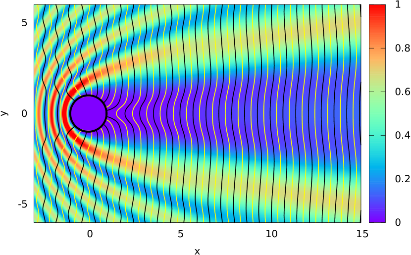
Figure 1: Color plot of the density (in arbitrary units) corresponding to the Green function (18) in the case of a hard disk scatterer of radius $a=1$. The incident wake vector is $\vec{k}=4.5\,a^{-1}\vec{e_{x}}$, corresponding to the situation studied in Ref. cilibrizzi ($ka=4.5$). The yellow solid lines are the lines of equiphases $0$ and $\pi$ and the black solid lines are the lines of equiphase $\pm\pi/2$.

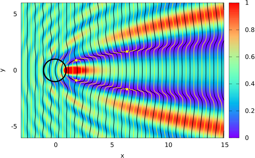
Figure 2: Same as Fig. 1 for an attractive potential with $2ma^{2}U_{0}/\hbar^{2}=-15$. The four yellow points are zeros of the wave function. They are approximately located at positions $(1.899,\pm 0.8928)$ and $(6.4056,\pm 1.674)$.

The diffraction pattern of Fig. 1 displays no noticeable structure: the wake of the (impenetrable) potential corresponds to the shadow of the obstacle and to a region of low density. On the other hand, in the case of a penetrable (attractive) potential, one sees a region of high density (for $x>0$ and $y\simeq 0$) separating two elongated regions of low density (cf. Fig. 2). These low density regions are similar to the ones observed in Ref. cilibrizzi and are located around zeros of the wave function. The zeros in Fig. 2 are indicated by four yellow points at which the yellow and black wavefront (respectively zeros of $\mathrm{Im}\,G$ and of $\mathrm{Re}\,G$) cross. They are associated to phase singularities, as we now discuss.

3 Wave singularities

While the scattering pattern of Fig. 1 has no noticeable structure, one sees zeros of the wave function in the wake of the obstacle of Fig. 2. They are easily located as points where the lines $\mathrm{Re}\,G=0$ and $\mathrm{Im}\,G=0$ cross. In a first part of this section we present the local behavior of $\psi$ around the nodal points, and in the second part we verify that the exact solution (18) has all the characteristic behaviors identified in Sec. 3.1.

3.1 Model Case

Let us denote as $X$ and $Y$ the abscissa and ordinate in a coordinate system whose origin is fixed at a nodal point of the wave function. We chose the $X$-axis in such a way that the wave field can be locally represented in the form

$$\psi\cong(\alpha X-{\rm i}Y)\,e^{{\rm i}kX},$$ (22)

that is, the wave is locally represented by a plane wave whose amplitude vanishes at the origin. The coefficient $\alpha>0$ controls the scales along the coordinate axes and the choice of signs is made for later convenience. As one can easily see, the density distribution

$$|\psi|^{2}=\alpha^{2}X^{2}+Y^{2}$$ (23)

has an elliptic form, and if $\alpha\ll 1$ the lines of constant density are strongly elongated along the $X$-axis. The phase has a more interesting behavior corresponding to an edge dislocation in the wave field nb-1974 . The phase $\theta$ of the wave function is defined by the equation

$$\theta(X,Y)=\arctan\frac{\alpha X\sin(kX)-Y\cos(kX)}{\alpha X\cos(kX)+Y\sin(kX)},$$ (24)

We show in Fig. 3 wavefronts (i.e., lines of constant phase) and streamlines which are the field lines of the vector field $\nabla\theta$ with

$$\theta_{X}=\frac{\alpha(Y+\alpha kX^{2})+kY^{2}}{|\psi|^{2}},\quad\theta_{Y}=-\frac{\alpha X}{|\psi|^{2}}.$$ (25)

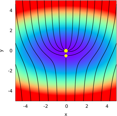
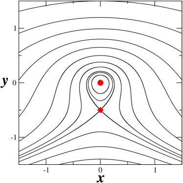
Figure 3: Left plot: color plot of the density corresponding to the wave function (22) ($\alpha=0.5$ and $k=1$). The blue (red) color corresponds to a region of lower (higher) density. The black solid lines are wavefronts ($\theta=0,\pm\pi/4,\pm\pi/2,\pm 3\pi/4\pi,\pi)$. The nodal point at the origin is marked by a yellow circle and the stagnation point (26) by a yellow diamond. Right plot: corresponding streamlines. Note that the scale (and the color of the singular points) has been modified in order to get a better resolution in the region near the origin.

One can see that the lines of constant phase stem from the origin and that the streamlines form circles around it. This means that there is a vortex located at the origin (the nodal point) and that the velocity field $\nabla\theta$ has a singularity here. There is another remarkable point where the backward velocity induced by the vortex just cancels the plane wave flow velocity $k\,\vec{e_{x}}$. This is a critical point of the vector field (25) with vanishing velocity $(\theta_{X},\theta_{Y})$. Its coordinates are given by

$$X=0\;,\quad Y=-\alpha/k\;.$$ (26)

It is easy to find that the Hessian has here opposite eigenvalues ($\pm\alpha^{3}/k^{2}$), meaning that this critical point is a saddle, as clearly seen in the left plot of Fig. 3. The separatrix going through the saddle point has a fixed phase which can be put equal to $\pi$, or equal to $\pi$ along one branch and equal to $-\pi\equiv\pi\mod(2\pi)$ along another branch. Therefore the phases of the wavefront at this point can change values between two choices equal to each other modulus $2\pi$ and the whole change of phase depends on the charge of the vortex located “inside” the separatrix line. In our case (Fig. 3) the phase changes from $-\pi$ at one branch of the separatrix to $\pi$ at the other branch (if one goes from left to right), that is the charge of the vortex is equal to unity.

As one can see, the edge phase singularity described here leads to a very elongated region of low density if $\alpha\ll 1$ [cf. (23)] which can mimic the experimental situation observed in Ref. cilibrizzi if the distance $k/\alpha$ is less than the typical distance between the “pseudo-soliton” and the incident flow axis. If this condition is not fulfilled, then we have to take into account the existence of a symmetrical edge phase singularity below the axis of the flow. This can be done by making the approximation that the angles between the “pseudo-solitons” and the axis of the flow are negligibly small. In this case we can approximate locally the solution of our scattering problem by the exact solution of the Helmholtz equation (see Refs. nb-1974 ; nye99 ; Nye88 )

$$\psi=\left[X-{\rm i}k(Y^{2}-b)\right]e^{{\rm i}kX}\;,$$ (27)

where $b$ is real. If $b$ is positive, this field has nodes at points $(0,\pm\sqrt{b})$ corresponding to vortices with opposite circulations. The corresponding velocity field $\nabla\theta$ has two stagnation points with coordinates $(X_{s},Y_{s})$

$$(X_{s},Y_{s})=\left\{\begin{array}[]{lcc}(0,\pm\sqrt{b-k^{-2}})&\text{if}&b>k^{-2},\\ (\pm\sqrt{b-k^{2}b^{2}},0)&\text{if}&b<k^{-2},\end{array}\right.$$ (28)

and it is easy to show that these are saddle points. Thus, for large enough values of $b$ the two vortices and the two saddle points are located on the $y$ axis and the resulting structure can be represented as a symmetrical combination of two edge phase dislocations with a shallow low density region of large horizontal extension (see the upper left plot of Fig. 4). When $b$ decreases, an interesting mechanism of collapse of the singularities occurs which is depicted in Fig. 4. For $b=k^{-2}$ (upper right plot) the saddle points collide at the origin and for decreasing $b$ they start to move symmetrically from the origin along the $x$ axis (lower left plot): after initially drifting apart, the two saddles get closer anew. At last, when $b=0$ all vortices and saddle points annihilate at the origin, the dislocation disappears and for $b<0$ the flow becomes regular (lower right plot).

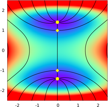
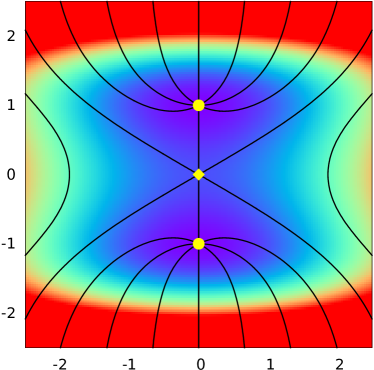
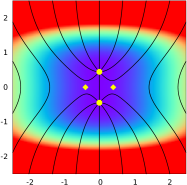
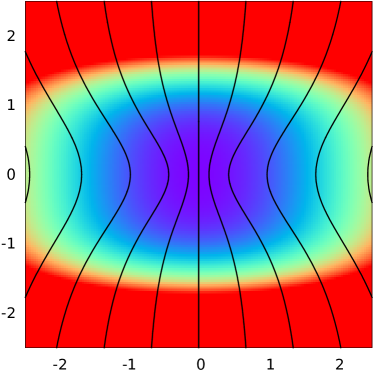
Figure 4: Plot of the intensity of the wave function (27) (with $k=1$) for different values of the parameter $b$ (from upper left to lower right: $b=2$, 1, $0.2$ and $-0.2$). The blue (red) color corresponds to a region of lower (higher) density. In each plot the black solid lines are the wavefronts $\theta=0,\pm\pi/4,\pm\pi/2,\pm 3\pi/4\pi,\pi$, the yellow circles are the nodal point and the diamonds are the saddle points.

This scenario of disappearance of the wave singularities was put forward by Nye, Hajnal and Hannay in Ref. Nye88 . It is robust because it obeys the restrictions dictated by topology, as we now explain. Two topological indices can be ascribed to the nodal and saddle points. One of them, known as the topological charge or vorticity $I_{\rm V}$, measures the circulation of the velocity field around the singularity: $I_{\rm V}=\pm 1$ around the nodes of the wave functions (22) and (27) and $I_{\rm V}=0$ around a saddle. The other one, known as Poincaré index $I_{\rm P}$, measures the change of direction of the equiphase lines around the singularity: $I_{\rm P}=1$ for a node and $I_{\rm P}=-1$ for a saddle. The simple annihilation of two vortices of opposite topological charge is not possible because it does not conserve the Poincaré index. In the Nye et al. scenario instead, the concomitant annihilation of the zeros and of the saddles conserve both the total vorticity and Poincaré index.

3.2 The wake of a penetrable disk

In our scattering problem the process just described is controlled by the parameters $U_{0}$ (the depth of the potential) and $k$ (the incident wave vector). We now show that this process is indeed observed when changing the parameters $U_{0}$ and $k$ starting from the situation depicted in Fig. 2. In view of a possible experimental implementation it is more appropriate to keep $U_{0}$ fixed and to change the value of the incident wave vector. Fig. 5 depicts the density pattern and the corresponding streamlines for $k=2.0/a$ (and $2ma^{2}U_{0}/\hbar^{2}=-15$).

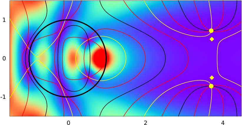
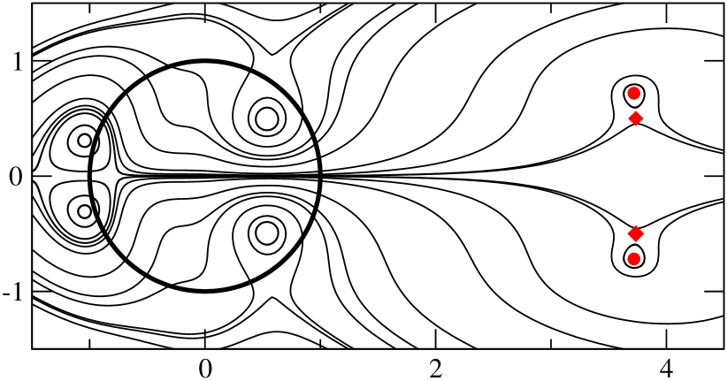
Figure 5: Upper plot: density of the wave function for a beam scattering onto a penetrable disk with $2ma^{2}U_{0}/\hbar^{2}=-15$. The horizontal (vertical) axis is the $x$-axis ($y$-axis) in units of $a$. The color code is the same as in Figs. 1 and 2. The incident wave vector is $\vec{k}=\frac{2.0}{a}\,\vec{e_{x}}$. The yellow solid lines are the lines of equiphases $0$ and $\pi$, the black solid lines are the lines of equiphase $\pm\pi/2$ and the purple solid lines are the lines of equiphase $\pm\pi/4$ and $\pm 3\pi/4$. Lower plot: streamlines. The nodes and saddles in the region $x\simeq 3.7$ are marked by yellow (red) points and diamonds in the upper (lower) plot. The positions of the other nodes and saddles are not marked by a special signs in the figure.

For this value of $k$ the zeros of the wave function in the wake of the obstacle are closer one to each other than in Fig. 2. One is in a situation similar to that shown in the upper left plot of Fig. 4: Two nodes and two saddles are almost aligned on a vertical lineremark_saddles in the region $x\simeq 3.7\,a$. If $k$ slightly decreases to $k=1.9/a$, one obtain the results depicted in Fig. 6: the two nodes still have symmetric positions with respect to the horizontal axis but the saddles now lay on this axis. This is a situation similar to the one depicted in the left lower plot of Fig. 4. Finally, for $k=1.8/a$ (not shown) the flow becomes regular in the region $x\simeq 3.7\,a$ and $y=0$: Hence the disappearance of the zeros and of the saddles in this region exactly follows the scenario of Nye, Hajnal and Hannay presented in the previous sub-section.

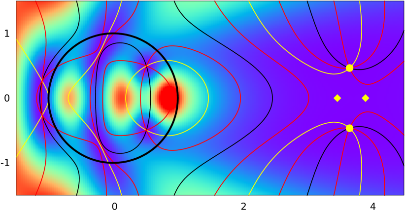
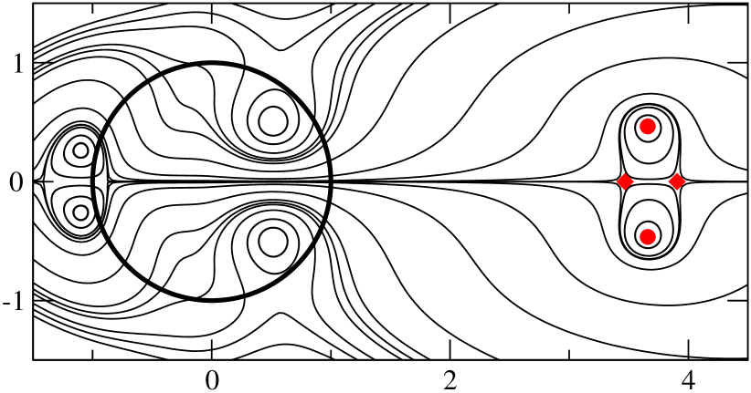
Figure 6: Same as Fig. 5 for $k=1.9/a$.

The detailed analysis just presented of the symmetrical regions of lower density in the wake of an attractive obstacle (depicted in Fig. 2) confirms the original discussion of Ref. cilibrizzi : these zones correspond to phase singularities in vicinity of zeros of the wave function. Indeed, the rapid change of the phase across these regions mimics the behavior of the phase across the oblique solitons observed in the wake of a nonlinear fluid.

However, there are marked differences between the linear phase singularities and the oblique solitons: (a) the phase singularities are not seen in the wake of an impenetrable obstacle (see Fig. 1); (b) the phase singularities are less robust, in the sense that they can easily disappear upon changing the incident wave vector or the depth of the potential, however, this disappearance is in itself an interesting phenomenon governed by topological constraints as just verified; (c) the phase singularities occupy only a finite region of the stationary interference pattern whereas the length of oblique solitons increases with time in principle ad infinitum (see Ref. kk-2011 ); (d) the width of an oblique soliton is controlled by the balance of the dispersion and nonlinearity whereas the characteristic size of the dark regions around the phase singularities depends on the parameters of the obstacle only (see the precise discussion in Section 5); (e) at last, the threshold wave number of the incident wave for appearance of oblique solitons is related with the characteristic sound velocity in the polariton condensate Kam08 ; kk-2011 whereas there is no such threshold for the formation of a linear interference pattern.

4 Resonant scattering

So far we have concentrated our attention on the wave pattern outside the obstacle where phase dislocations can be formed which are accompanied by elongated dips in the density distributions. However, the exact solution (21), (15) provides also valuable informations about the wave distribution inside the region occupied by the obstacle.

4.1 Low energy scattering

A first interesting situation occurs for low energy scattering on an attractive potential ($U_{0}<0$). One works in the low incident energy regime where $ka\ll 1$ and $\hbar^{2}k^{2}/2m\ll|U_{0}|$. In this case one can show that the coefficients $\tilde{B}_{n}$ of the partial wave expansion in (15) behave as $(ak)^{2n}$ and only the $s$-wave contributes significantly to the scattering.

It is convenient to measure the depth of the potential well in units of a wave vector $Q_{0}$ defined by

$$\frac{\hbar^{2}Q_{0}^{2}}{2\,m}=|U_{0}|\;.$$ (29)

In this case, defining the quantity $\kappa$ by

$$\ln\left(\frac{\kappa\,a\,e^{\gamma}}{2}\right)=\frac{1}{Q_{0}a}\,\frac{J_{0}(Q_{0}a)}{J_{0}^{\prime}(Q_{0}a)}\;,$$ (30)

where $\gamma$ is the Euler-Mascheroni constant, and using the asymptotic expansions of Hankel and Bessel functions for small argument AS one obtains from (15):

$$\tilde{B}_{0}\simeq\frac{-1}{1+\frac{2{\rm i}}{\pi}\ln(k/\kappa)}\;.$$ (31)

A similar expression is generally valid for any low energy scattering process in two dimensionsLL-3 . Eq. (31) also applies for a repulsive potential, but in this case the definition (30) of $\kappa$ should be replaced by (40). In the case of a hard disk scatterer for instance, the constant $\kappa$ takes the value $\kappa=2e^{-\gamma}/a$: this can be obtained by taking the limit $U_{0}\to+\infty$ in (40), or directly from the expression (20). In the attractive case which we consider in the present sub-section, $\kappa$ has the following physical meaning: if there is a bound $s$-state close the thresholdremark6 , i.e., if one is in the case of quasi-resonant scattering, then this state has an energy $-\hbar^{2}\kappa^{2}/(2m)$.

From (31) one sees that the cross section

$$\sigma=\int_{0}^{2\pi}|f(\varphi)|^{2}{\rm d}\varphi\stackrel{{\scriptstyle ka\to 0}}{{\simeq}}\frac{4}{k}\,|\tilde{B}_{0}|^{2}\;,$$ (32)

diverges at low energy. Thus, in this limit, the linear scattering process is markedly different from the nonlinear one for which superfluidity prevails at low incident velocity. Actually this is again the manifestation of the existence of an important characteristic quantity of the polariton condensate, namely the velocity of sound: scattering disappears for a nonlinear flow whose velocity is lower than the critical velocity which – in weakly interacting polariton gas – is of the order of the sound velocity pol-super .

4.2 Quasi-stationary states over a repulsive potential

The scattering amplitude (15) has poles for complex values of the variable $k$ and this means that quasistationary states can be formed under certain conditions. It is interesting to consider such a possibility here because these states can be detected experimentally.

The poles correspond to zeroes of the denominator in the expression (15) of the scattering amplitude, that is they are determined by the equation

$$k_{0}J_{n}^{\prime}(k_{0}a)H_{n}^{(1)}(ka)=kJ_{n}(k_{0}a)H_{n}^{(1)\prime}(ka).$$ (33)

This equation has, generally speaking, complex roots with comparable real and imaginary parts. However, for observing a long living quasistationary state the imaginary part must be much smaller than the real one. Such a configuration appears if the repulsive potential (3) is large enough,

$$U_{0}\gg\frac{\hbar^{2}}{ma^{2}},$$ (34)

and if the kinetic energy of incident polaritons is only slightly greater than $U_{0}$:

$$\frac{\hbar^{2}k^{2}}{2m}-U_{0}\ll U_{0}\;.$$ (35)

Then we see from Eq. (9) that in this case $k_{0}\ll k$ and the left hand side of Eq. (33) is small, hence $J_{n}(k_{0}a)$ must be accordingly small. This occurs if $k_{0}a$ is close to a zero of the Bessel function $J_{n}(z)$. If, for instance, $k_{0}a$ is close to the value $j_{n,s}$ of the $s^{\rm th}$ zero of $J_{n}$,

$$k_{0|n,s}a=j_{n,s}+\delta_{n,s}\quad(\,\mbox{with}\;|\delta_{n,s}|\ll 1\,)\;,$$ (36)

then, an expansion of Eq. (33) with respect to the small parameters $\delta_{n,s}$ and $k_{0|n,s}/k$ yields in the leading approximation the following expression for $\delta_{n,s}$ :

$$\delta_{n,s}\simeq\frac{j_{n,s}}{Q_{0}a}\,\frac{H_{n}^{(1)}(Q_{0}\,a)}{H_{n}^{(1)\prime}(Q_{0}\,a)}\;,$$ (37)

where $Q_{0}$ is defined by Eq. (29). As one can see, the imaginary part of $k_{0|n,s}$ (as well as the correction to the real part) is of order of $\sim(Q_{0}a)^{-1}$ and is small at least for the first quasistationary levels provided the condition (34) is fulfilled. Thus, for observing a quasistationary level, the wavenumber inside the obstacle should be equal to the complex eigenvalue $k_{0|n,s}$ determined by Eq. (36). From the relationship $k_{0|n,s}^{2}=k_{n,s}^{2}-Q_{0}^{2}$ we find in the leading approximation the resonance values of the wave vector $k$ of the incident wave:

$$k_{n,s}a\equiv(k_{n,s}^{\prime}+{\rm i}\,k_{n,s}^{\prime\prime})a\approx Q_{0}a+\frac{1}{2}\,\frac{j_{n,s}^{2}}{Q_{0}a}+{\rm i}\,\frac{j_{n,s}\delta_{n,s}^{\prime\prime}}{Q_{0}a},$$ (38)

where $\delta_{n,s}\equiv\delta_{n,s}^{\prime}+{\rm i}\,\delta_{n,s}^{\prime\prime}$ and the contribution of the real part $\delta_{n,s}^{\prime}$ has been neglected with respect to larger contributions of order $\sim(Q_{0}a)^{-1}$.

As an illustration, we consider a repulsive potential for which the parameters $U_{0}$ and $a$ are related by $2ma^{2}U_{0}/\hbar^{2}=60=(Q_{0}a)^{2}$ [thus verifying the condition (34)]. We look for instance for the first resonance in the $s$-wave channel, i.e., we consider a configuration where $k_{0}a$ is close to the first zero of $J_{0}$: $j_{0,1}=2.40482555...$. Formulas (36), (37) and (38) yield $\mbox{Re}\,(k_{0|0,1}a)\simeq 2.385$ and $\mbox{Re}\,(k_{0,1}a)\simeq 8.12$. The expected resonance is indeed observed for this value of the incident wave vector, as shown in Fig. 7: in this case the density of the scatterer wave has a strong maximum at the center of the repulsive disk. In Fig. 8 we display the first resonance in the $n=1$ channel. In this case formula (38) yields $\mbox{Re}\,(k_{1,1}a)\simeq 8.69$ and one observes a non-isotropic intensity pattern inside the circle, typical for a $p$-state.

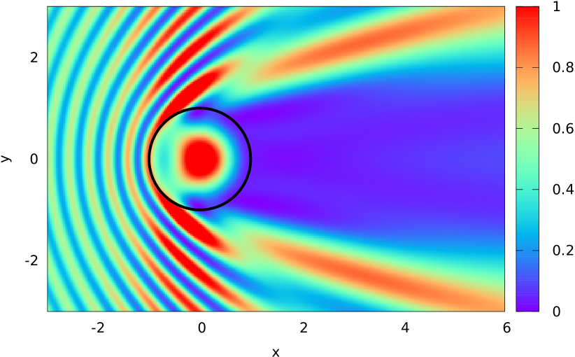
Figure 7: Density of the wave function scattered by a repulsive disk with $2ma^{2}U_{0}/\hbar^{2}=60$. The incident wave vector is $k\,a=8.12$ in order to meet the requirement of quasi-resonance in the $s$ channel (cf. the discussion in the text).

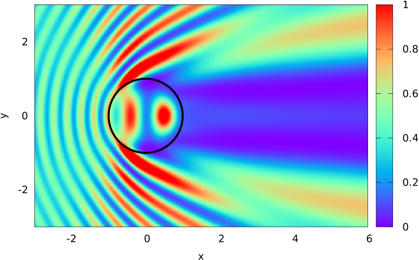
Figure 8: Same as Fig. 7 for an incident wave vector $k\,a=8.69$.

The cross section

$$\sigma(k)=\frac{1}{4\,k}\sum_{n=-\infty}^{+\infty}|\tilde{B}_{n}|^{2}$$ (39)

for the potential corresponding to Figs. 7 and 8 (for which $2ma^{2}U_{0}/\hbar^{2}=60$) is represented in Fig. 9. In this figure the dashed line is the low energy approximation (32) of the cross section, where $\tilde{B}_{0}$ is given by (31) with $\kappa$ being here defined as

$$\ln\left(\frac{\kappa\,a\,e^{\gamma}}{2}\right)=\frac{1}{Q_{0}a}\,\frac{I_{0}(Q_{0}a)}{I_{0}^{\prime}(Q_{0}a)}\;,$$ (40)

which is the version of Eq. (30) appropriate for a repulsive potential ($I_{0}$ being the modified Bessel function AS ). The two resonances we have identified are marked with arrows in the figure. One corresponds to a minimum of the cross-section and the other one to a maximum, following Fano mechanism.

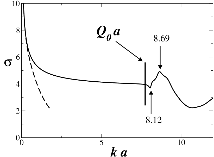
Figure 9: Cross section $\sigma(k)$ for a repulsive potential with $2ma^{2}U_{0}/\hbar^{2}=60$. The two arrows mark the resonances corresponding to the intensity patterns displayed in Fig. 7 and 8: respectively $ka=\mbox{Re}\,(k_{0,1}a)\simeq 8.12$ and $ka=\mbox{Re}\,(k_{1,1}a)\simeq 8.69$. The dashed line is the low energy approximation described in the text [Eqs. (32), (31) and (40)]. The vertical line locates the threshold wavenumber above which $\hbar^{2}k^{2}/(2m)>U_{0}$.

5 Conclusion

In optics one usually devotes a special attention to bright regions with high intensity of light: focuses, caustics, but also resonances as in Fig. 7 and 8. Another type of singularities appears in faint light, i.e., close to the dark spots where nodes of the light field are associated to phase dislocations. In these zones, complicated phase patterns may occur, with sharp changes (“jumps”) of phase across certain lines. We believe that such a linear optics phenomenon was observed in the experiment of Cilibrizzi et al cilibrizzi .

We have described how the dark elongated valleys observed in the wake of an attractive obstacle [Ref. cilibrizzi and Fig. 2] can merge and disappear upon changing the incident wave-vector and/or the depth of the potential. This phenomenon is accounted for within a fully linear theory and follows a typical scenario first proposed in Ref. Nye88 . As a side result, this shows that the occurrence of a bright region separating two dark elongated valleys in the wake of the obstacle is not generic. In particular, contrarily to oblique solitons, it is not observed in the wake of an impenetrable disk.

The applicability of the approach of the present work is limited by nonlinear effects caused by the interaction between polaritons. Considering the interest raised by the observation of phase defects in optics optics-singularities , in Bose-Einstein condensates BEC-singulatities , in polariton condensates cilibrizzi ; Fla13 and in other fields Boa06 , it is appropriate to set up simple criteria making it possible to discriminate the linear wake from the nonlinear one and to discuss how nonlinearity affects the structures presented in this article.

As discussed above, there are marked qualitative differences between the linear an the non-linear case: the low velocity behavior of the flows are quite different (superfluid in the nonlinear case and, at variance, a diverging cross section in the linear case). Also the comparison between scattering from an impenetrable and a penetrable defect shows that, whereas the nonlinear wake is expected in both cases to lead to the formation of oblique solitons, in the linear regime the dark streaks only appear when the defect is penetrable (cf. Figs. 1 and 2). Our analysis also provide another qualitative criterion making it possible to distinguish an oblique soliton from a dip in a linear wake: the linear dip is associated to a phase singularity, and the phase of the wave function varies rapidly when crossing the low density region. This change of phase corresponds to a minimum or a maximum in the region between the streaks depending on which side of the singularity one considers. This is already clear from Fig. 2 and made explicit in Fig. 10: along the red dashed line drawn in this figure, the phase is decreased between two low density regions, whereas along the blue dashed path the phase is higher when $y\approx 0$. The situation is quite different for an oblique soliton in the wake of a nonlinear flow, as can be understood from the following remarks: (i) the phase of a dark soliton of the Gross-Pitaevskii equation increases in the direction opposite to its direction of propagation; (ii) an oblique soliton is stationary because its transverse velocity, related with the phase jump, is locally compensated by a component of the incident flow velocity. As a result of properties (i) and (ii) the phase always increases between the low density streaks delimited by two oblique solitons, as proved theoretically in Refs. egk-2006 ; Kam08 ; kk-2011 . Since the phase is measurable in polariton experiments, this criterion can be implemented in principle in the analysis of experimental data: nonlinear oblique solitons can be identified from the fact that the phase always increases between the low density streaks.

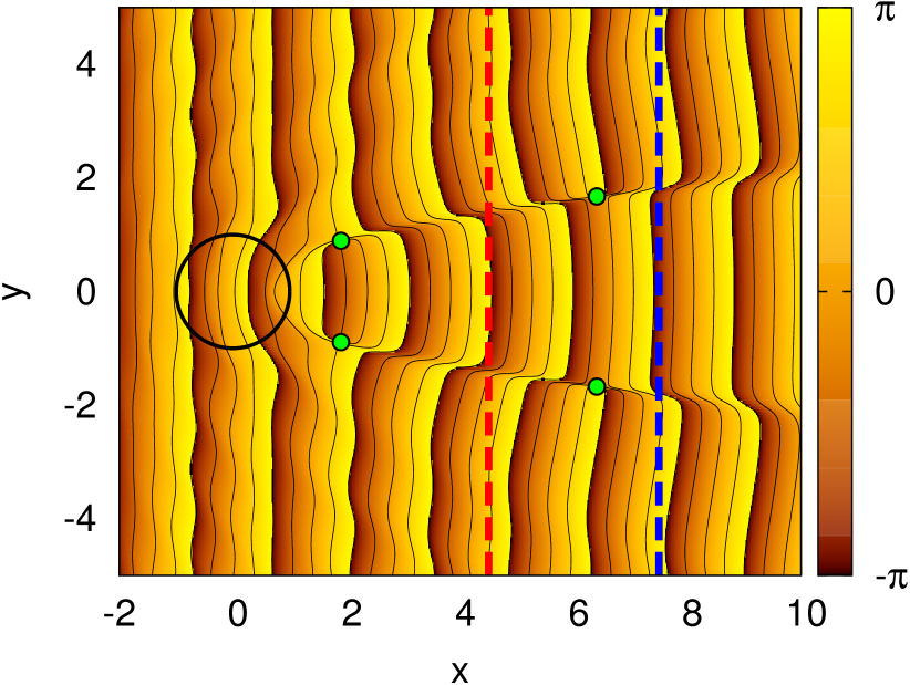
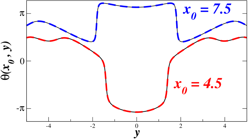
Figure 10: Upper part: color plot of the phase $\theta(x,y)={\rm arg}\,[\psi(x,y)]$ for the same potential as in Fig. 2 (with also $a=1$ and $\vec{k}=4.5\,\vec{e}_{x}$). The green dots are zeros of the wave function. Lower part: detailed plot of the evolution of the phase of the wave function along the paths displayed in the upper plot as red and blue dashed lines (located at $x_{0}=4.5$ and 7.5).

Note also that, in addition to this qualitative discussion, it is very instructive to perform a quantitative analysis of the change of the width of the dark strips with the distance from the defect in the linear and in the nonlinear cases. Studies of this type, with corresponding experimental data, are presented in the supplementary material of Refs. cilibrizzi and amo-2011 .

We now present quantitative estimates making it possible to evaluate the importance of nonlinear effects in the structures of the wake observed behind an obstacle. Working in the standard mean field approach, interaction effects are most easily accounted for by replacing the effective Schrödinger equation (1) by the Gross-Pitaevskii equation:

$${\rm i}\,\hbar\,\psi_{t}=-\frac{\hbar^{2}}{2m}\nabla^{2}\psi+\left[U(\vec{r})+g|\psi|^{2}\right]\psi\;,$$ (41)

where $g$ denotes the effective interaction constant (related to the $s$-wave scattering length which characterizes the low-energy inter-particle scattering). The linear effects dominate if the characteristic size $d$ of the diffraction pattern (say, the width of the dip around a node) is much less than the healing length $\xi$,

$$d\ll\xi,$$ (42)

where the healing length is defined as

$$\xi=\frac{\hbar}{\sqrt{2mg\rho_{0}}}\,,$$ (43)

and $\rho_{0}$ is the characteristic density of the polariton gas. To obtain a rough estimate of the size $d$, we can use the result of the Born approximation (8) which yields a scattering amplitude of the order $f\sim(Q_{0}a)^{2}/\sqrt{k}$ and a characteristic angle $\varphi\sim(ak)^{-1}$. The phase singularity appears at a distance

$$x\sim f^{2}\sim(Q_{0}a)^{4}/k$$ (44)

and the characteristic width of the dip is

$$d\sim x\,\varphi\sim\frac{(Q_{0}a)^{4}}{k^{2}a}\;.$$ (45)

Thus, if the parameters characterizing the obstacle and if the incident wave number are such that this estimate of $d$ satisfies the condition (42), then the wave pattern is formed by purely linear interference effects; otherwise the nonlinear effects prevail in the formation of the wake structure in the flow.

As an illustration of the experimental relevance of this type of quantitative estimate we return to the above discussion where we stated that nonlinear oblique solitons can in principle be identified from the fact that the phase always increases between the low density streaks. For using this criterion in practice one has to measure the sign of the phase jump along a long enough segment of the experimentally observed dip: precisely along a length greater than the estimate $x$ in Eq. (44) in order to make sure that the region around a possible point of the phase singularity is not missed in the measurements.

One should also notice that for increasing incident polaritons density, the linear wave pattern discussed here transforms gradually into the so-called “ship wave” structure ship-1 ; ship-2 located outside the Mach cone. On the contrary, the nonlinear oblique solitons discussed in Refs. egk-2006 ; Kam08 ; amo-2011 ; grosso-2011 are located inside the Mach cone. Combining this remark with the above estimates permits one to distinguish the most important physical effects which are responsible for the wave pattern observed in the experiments.

- (1) P. Cilibrizzi, H. Ohadi, T. Ostatnicky, A. Askitopoulos, W. Langbein and P. Lagoudakis, Phys. Rev. Lett. 113, (2014) 103901.
- (2) G. A. El, A. Gammal, A. M. Kamchatnov, Phys. Rev. Lett. 97, (2006) 180405.
- (3) A. M. Kamchatnov and L. P. Pitaevskii, Phys. Rev. Lett. 100, (2008) 160402.
- (4) A. Amo, S. Pigeon, D. Sanvitto, V. G. Sala, R. Hivet, I. Carusotto, F. Pisanello, G. Lemenager, R. Houdré, E. Giacobino, C. Ciuti, A. Bramati, Science 332, (2011) 1167.
- (5) G. Grosso, G. Nardin, F. Morier-Genoud, Y. Léger, B. Deveaud-Plédran, Phys. Rev. Lett. 107, (2011) 245301.
- (6) A. Amo, J. Bloch, A. Bramati, I. Carusotto, C. Ciuti, B. Deveaud-Plédran, E. Giacobino, G. Grosso, A. Kamchatnov, G. Malpuech, N. Pavloff, S. Pigeon, D. Sanvitto, D. D. Solnyshkov, Comment on “Linear wave dynamics explains observations attributed to dark-solitons in a polariton quantum fluid”, arXiv:1401.7347.
- (7) J. F. Nye, Natural Focusing and Fine Structure of Light: Caustics and Wave Dislocations, CRC Press (1999).
- (8) M. S. Soskin and M. V. Vasnetsov, Singular optics, in Progress in Optics vol. 42, (2001) 219.
- (9) J. F. Nye and M. V. Berry, Proc. Roy. Soc. Lond. 336, (1974) 165.
- (10) M. Born and E. Wolf, Principles of Optics, Cambridge University Press (Cambridge, 1999).
- (11) M. V. Berry, in “Second international conference on Singular Optics (Optical Vortices): Fundamentals and applications” SPIE 4403 (Bellingham Washington, 2001), pp 1-12.
- (12) L. D. Landau and E. M. Lifshitz, Quantum Mechanics, Pergamon, Oxford, 1977.
- (13) Lord Rayleigh, Theory of Sound, Vol. 2, Macmillan, 1896.
- (14) Lord Rayleigh, Phil. Mag., S.6, 36, (1918) 365.
- (15) M. Abramowitz and I. A. Stegun, Handbook of Mathematical Functions, Dover, New York, 1972.
- (16) I. Carusotto and G. Rousseaux in “Analog Gravity Phenomenology”, D. Faccio et al. (eds.) Lecture Notes in Physics 870, pp 109-144, Springer International Publishing (Switzerland, 2013).
- (17) J. F. Nye, J. V. Hajnal, and J. H. Hannay, Proc. Roy. Soc. Lond., 417, (1988) 7.
- (18) The position of the nodes is easily determined from the upper plot of Fig. 5 which represents the density of the wave function and the wavefronts. On the other hand, the position of the saddles is more precisely determined from the plot of the streamlines (lower part of the figure).
- (19) A. M. Kamchatnov and S. V. Korneev, Phys. Lett. A 375, (2011) 2577.
- (20) A. Amo, J. Lefrère, S. Pigeon, C. Adrados, C. Ciuti, I. Carusotto, R. Houdré, E. Giacobino and A. Bramati, Nature Phys. 5, (2009) 805.
- (21) We recall that in two dimensions an attractive potential always has at least one bound state. The case of resonant scattering occurs when the energy of the highest bound state is close to threshold.
- (22) N. R. Heckenberg, R. McDuff, C. P. Smith, and A. G. White, Opt. Lett. 17, (1992) 221; J. Leach and M. J. Padgett, New J. Phys. 5, (2003) 154; W.M. Lee, X.-C. Yuan, and K. Dholakia, Opt. Commun. 239, (2004) 129; F. Flossmann, U. T. Schwarz, M. Maier, and M. R. Dennis, Phys. Rev. Lett. 95, (2005) 253901; T. A. Fadeyeva, V. G. Shvedov, Y. V. Izdebskaya, A. V. Volyar, E. Brasselet, D. N. Neshev, A. S. Desyatnikov, W. Krolikowski, and Y. S. Kivshar, Opt. Express 18, (2010) 10848.
- (23) E. L. Bolda and D. F. Walls, Phys. Rev. Lett. 81, (1998) 5477; J. Tempere and J. T. Devreese, Solid State Commun. 108, (1998) 993; S. Inouye, S. Gupta, T. Rosenband, A. P. Chikkatur, A. Görlitz, T. L. Gustavson, A. E. Leanhardt, D. E. Pritchard, and W. Ketterle, Phys. Rev. Lett. 87, (2001) 080402; F. Chevy, K. W. Madison, V. Bretin, and J. Dalibard, Phys. Rev. A, 64, (2001) 031601(R); S. Stock, Z. Hadzibabic, B. Battelier, M. Cheneau, and J. Dalibard, Phys. Rev. Lett. 95, (2005) 190403.
- (24) H. Flayac, D. D. Solnyshkov, I. A. Shelykh, and G. Malpuech, Phys. Rev. Lett. 110, (2013) 016404.
- (25) A. D. Boardman, Yu. G. Rapoport, V. V. Grimalsky, B. A. Ivanov, S. V. Koshevaya, L. Velasco, and C. E. Zaspel, Phys. Rev. E 71, (2005) 026614.
- (26) I. Carusotto, S. X. Hu, L. A. Collins, and A. Smerzi, Phys. Rev. Lett. 97, (2006) 260403.
- (27) Yu. G. Gladush, G. A. El, A. Gammal, and A. M. Kamchatnov, Phys. Rev. A 75, (2007) 033619.