Impact of small scale inhomogeneities
on observations of standard candles

Abstract

We investigate the effect of small scale inhomogeneities on standard candle observations, such as type Ia supernovae (SNe) observations. Existence of the small scale inhomogeneities may cause a tension between SNe observations and other observations with larger diameter sources, such as the cosmic microwave background (CMB) observation. To clarify the impact of the small scale inhomogeneities, we use the Dyer-Roeder approach. We determined the smoothness parameter $\alpha(z)$ as a function of the redshift $z$ so as to compensate the deviation of cosmological parameters for SNe from those for CMB. The range of the deviation which can be compensated by the smoothness parameter $\alpha(z)$ satisfying $0\leq\alpha(z)\leq 1$ is reported. Our result suggests that the tension may give us the information of the small scale inhomogeneities through the smoothness parameter.

I Introduction

The modern cosmology has achieved great success based on the cosmological principle, which states that our universe is homogeneous and isotropic on large scales such as over 100Mpc. It is widely believed that the universe is well approximated by the Friedmann-Lemaître-Robertson-Walker (FLRW) model over this scale. Cosmological parameters are estimated from observational data such as the type Ia supernovae (SNe) and the cosmic microwave background (CMB). Some tensions between independent observational data are often reported, e.g. the matter density parameter from SNe tends to be smaller than that from CMB. The tensions are more seriously considered than before due to recent progress of the observational accuracy. The reason for a tension would be a systematic error which originates from instruments or analysis, but it would be an unknown physical effect which may reveal the new physics and discovery. In this work, we propose use of such kinds of tension to obtain information about small scale inhomogeneities.

As we mentioned, it has been reported that there is a tension between SNe observations and CMB observations Ade:2013zuv . This tension would originate from small scale inhomogeneities as is reported in Refs. Fleury:2013uqa ; Fleury:2013sna . The real universe is inhomogeneous on the scales smaller than 100Mpc. It should be noted that the structure of the universe on the scales $\lesssim 10$kpc is unclear not only theoretically but also observationally. The theoretical difficulty mainly comes from nonlinear features of basic equations. Numerical simulations cost more to take the small scale inhomogeneities into account. On the other hand, observational investigation into much smaller scale inhomogeneities would be possible by using distant small diameter sources as probes. For instance, the typical diameter of SNe explosion is $10^{15}$cm. Therefore SNe can be regarded as point sources in cosmological observations.

In this paper, we focus on the comparison between SNe observations and other observations with much larger diameter sources, such as CMB observations. The observations of CMB is mainly affected by the large scale inhomogeneities and the influence from them can be estimated by using the perturbation theory. On the other hand, the observations of SNe may be significantly affected by the small scale inhomogeneities as well as the large scale ones. The effect of the inhomogeneities on the SNe observations is often estimated by using a ray shooting method with conventional models of inhomogeneity, and it is suggested that the inhomogeneities do not significantly affect the cosmological parameter estimation. However, as is mentioned before, we do not have any reliable inhomogeneity model in the scale of the diameter of SNe, i.e. $10^{15}$cm. Therefore, in the precision cosmology era, it is important to estimate the impact of the inhomogeneities without any bias.

In oder to estimate the effect of the small scale inhomogeneities, as a first step, we use the simplest approximation method: the Dyer-Roeder (DR) approach DR1 ; DR2 . In this approach, we introduce a new parameter $\alpha$, which characterizes the small scale inhomogeneities. The parameter $\alpha$ is called the smoothness parameter and it is defined such that the fraction $\alpha$ of the matter is smoothly distributed, while the fraction $1-\alpha$ is bound in clumps. The light propagation is only affected by the smoothly distributed matter if we assume that the bundles of light lays propagate far from all the clumps. The validity of the DR approach is discussed in Ref. Fleury:2014gha . Observational constraints on the value of $\alpha$ is discussed in e.g. Ref. BSL1 and references therein. In those analysis, $\alpha$ is assumed to be constant. However, the smoothness parameter does not necessarily have to be constant. The redshift dependence of the smoothness parameter was first discussed by Linder Linder1 ; Linder2 .

We consider the smoothness parameter is in the interval $0\leq\alpha(z)\leq 1$ from its definition(but see Ref.Lima:2013rs for $\alpha>1$ cases). The redshift dependence of the smoothness parameter should be related to the history of the structure formation of our universe. Naively thinking, the value of the smoothness parameter decreases with the progress of the structure formation. Therefore, the smoothness parameter is expected to be monotonically increasing function of the redshift. In addition, since the early universe was totally homogeneous, it should asymptote to unity as $z\rightarrow\infty$.

Hereafter, we rely on the “opacity hypothesis” proposed in Ref. Fleury:2013sna . This hypothesis states that all observed SNe have passed through the region far from clumps. It might be justified by the following reasonsFleury:2013sna : the probability of passing through near clumps is too small, clumps may be bright enough to hide SNe behind it, strong gravitational lensing due to a clump makes it so bright that it is regarded as isolated exceptional source. Throughout this paper, we assume that the distance redshift relation of SNe is given by the DR distance with true cosmological parameters which describe global aspect of the universe.

In this paper, we demonstrate the impact of the inhomogeneities in the following way. We consider two sets of cosmological parameters which are taken from SNe observation ($\Omega^{\rm SNe},w^{\rm SNe}$) and another observation with larger source diameter, such as CMB anisotropy observation ($\Omega^{\rm CMB},w^{\rm CMB}$). We regard the cosmological parameters determined by the SNe observation are fictitious since the effect of the small scale inhomogeneities is not taken into account. Assuming the other set of cosmological parameters correctly describes the global aspect of our universe, we determine the smoothness parameter $\alpha(z)$ as a function of the redshift so that it compensates the deviation of ($\Omega^{\rm SNe},w^{\rm SNe}$) from ($\Omega^{\rm CMB},w^{\rm CMB}$). If the fixed smoothness parameter has the desired feature as a function of the redshift, it implies that the tension between ($\Omega^{\rm SNe},w^{\rm SNe}$) and ($\Omega^{\rm CMB},w^{\rm CMB}$) can be explained by the effect of the small scale inhomogeneities. At the same time, the tension gives us the information of the small scale inhomogeneities through the smoothness parameter.

This paper is organized as follows. In Sec. II, we briefly review the DR approach and derive the DR equation. How to determine the redshift dependent smoothness parameter is described in Sec. III. In Sec. IV, we show the behavior of the smoothness parameter as a function of the redshift, and Sec. V is devoted to a summary.

In this paper, we use the geometrized units in which the speed of light and Newton’s gravitational constant are one, respectively.

II Dyer-Roeder equation

We assume that the universe is well described by the Friedmann-Lemaître-Robertson-Walker (FLRW) model on the large scale. The Robertson-Walker metric is given by

$$\mathrm{d}s^{2}=\mathrm{d}t^{2}-a^{2}(t)\left\{\frac{\mathrm{d}r^{2}}{1-kr^{2}}+r^{2}(\mathrm{d}\theta^{2}+\sin^{2}\theta\mathrm{d}\phi^{2})\right\},$$ (1)

where $a(t)$ is the scale factor, $k$ is the constant curvature. We consider non-relativistic matter and dark energy as energy components of the universe. The dark energy equation of state is given by $p_{\rm de}=w\rho_{\rm de}$, where $p_{\rm de}$ and $\rho_{\rm de}$ are the pressure and the energy density of the dark energy, respectively. The energy-momentum tensor has the form of a perfect fluid:

$$T^{\alpha\beta}=\left(\rho_{\rm m}+\rho_{\rm de}+p_{\rm de}\right)U^{\alpha}U^{\beta}-p_{\rm de}g^{\alpha\beta},$$ (2)

where $\rho_{\rm m}$ is the energy density of the non-relativistic matter and $U^{\alpha}$ is the 4-velocity of a comoving volume element. From the Friedmann equation, the Hubble parameter is given by

$$H(z) = H_{0}\sqrt{\Omega_{\rm m}(1+z)^{3}+\Omega_{\rm de}(1+z)^{3(1+w)}+\Omega_{\rm k}(1+z)^{2}}$$ (3)

$$\equiv H_{0}F(z;w,\Omega_{\rm m},\Omega_{\rm de},\Omega_{\rm k}),$$

where $H_{0}$ is the Hubble constant, $\Omega_{\rm m}$ and $\Omega_{\rm de}$ are the density parameter of the non-relativistic matter and the dark energy, respectively, and $\Omega_{\rm k}$ satisfies the equation

$${\Omega_{\rm m}}+{\Omega_{\rm de}}+{\Omega_{\rm k}}=1.$$ (4)

The Dyer-Roeder equation is based on the Sachs optical equationSachs :

$$\frac{\mathrm{d}^{2}}{\mathrm{d}v^{2}}\sqrt{A} = -\frac{1}{2}R_{\alpha\beta}k^{\alpha}k^{\beta}\sqrt{A},$$ (5)

where $v$ is the affine parameter, $A$ is the cross-sectional area of a light ray bundle, $R_{\alpha\beta}$ is the Ricci tensor and $k^{\alpha}$ is the null generator of the light rays. Here, we have neglected the shear term (see e.g.1992grle.book…..S ; sasaki ). According to the field equation, we can replace the Ricci tensor by the energy-momentum tensor as follows:

$$\frac{\mathrm{d}^{2}}{\mathrm{d}v^{2}}\sqrt{A} = -4\pi T_{\alpha\beta}k^{\alpha}k^{\beta}\sqrt{A}$$ (6)

$$= -4\pi(\rho_{\rm m}+\rho_{\rm de}+p_{\rm de})(U_{\alpha}k^{\alpha})^{2}\sqrt{A}.$$

Using the differential relation between the redshift and the affine parameter

$$\frac{\mathrm{d}z}{\mathrm{d}v}=(1+z)^{2}F(z;w,\Omega_{\rm m},\Omega_{\rm k}),$$ (7)

and the fact that the angular diameter distance is proportional to $\sqrt{A}$, we rewrite equation (5) as

$$F(z)\frac{\mathrm{d}}{\mathrm{d}z}\Bigl{\{}(1+z)^{2}F(z)\frac{\mathrm{d}}{\mathrm{d}z}{D}_{\rm A}(z)\Bigr{\}}$$ (8)

$$\hskip 85.35826pt+\frac{3}{2}\big{\{}\Omega_{\rm m}(1+z)^{3}+\Omega_{\rm de}(1+w)(1+z)^{3(1+w)}\big{\}}{D}_{\rm A}(z)=0,$$ (9)

where $\Omega_{\rm de}$ is given by $1-\Omega_{\rm m}-\Omega_{\rm k}$. Since this equation depends on the parameters $w$, $\Omega_{\rm m}$ and $\Omega_{\rm k}$, we use the following expression:

$$D_{A}(z)=D_{A}(z;w,\Omega_{\rm m},\Omega_{\rm k}).$$ (10)

In order to take account of small scale inhomogeneities, we introduce the smoothness parameter $\alpha(z)$ which describes the fraction of the smoothly distributed matter for each redshift. The fraction $1-\alpha(z)$ of the matter is clumped. The case of $\alpha=1$ corresponds to a totally homogeneous universe, while for $\alpha=0$ all the matter is clumped. From the definition of the smoothness parameter, it is reasonable to consider only the interval

$$0\leq\alpha(z)\leq 1.$$ (11)

If a bundle of light rays passes through far away from the clumped regions, the light rays feel the gravitational field of the smoothly distributed matter. Therefore, we replace the $\rho_{\rm m}$ in the energy-momentum tensor (2) by $\alpha(z)\rho_{\rm m}$. As a result, $\Omega_{\rm m}$ in the equation (9) is replaced by $\alpha(z)\Omega_{\rm m}$ and we get the Dyer-Roeder equation:

$$F(z)\frac{\mathrm{d}}{\mathrm{d}z}\Bigl{\{}(1+z)^{2}F(z)\frac{\mathrm{d}}{\mathrm{d}z}{D}_{\rm DR}(z)\Bigr{\}}$$ (12)

$$\hskip 85.35826pt+\frac{3}{2}\big{\{}\alpha(z)\Omega_{\rm m}(1+z)^{3}+\Omega_{\rm de}(1+w)(1+z)^{3(1+w)}\big{\}}{D}_{\rm DR}(z)=0,$$ (13)

where $D_{\rm DR}(z)$ is the Dyer-Roeder distance. Since the Dyer-Roeder distance depends on the cosmological parameters and the smoothness parameter, we use the following expression:

$$D_{\rm DR}(z)=D_{\rm DR}(z;w,\Omega_{\rm m},\Omega_{\rm k},\alpha(z)).$$ (14)

The boundary conditions for $D_{\rm A}$ and $D_{\rm DR}$ are given by

$$\begin{cases}\left.D\right|_{z=0}=0,\\ \left.\frac{\mathrm{d}D}{dz}\right|_{z=0}=1/H_{0}.\end{cases}$$ (15)

III Determination of $\alpha(z)$

In this section, we explain the procedure to determine the smoothness parameter from observation. As is mentioned in the introduction, we consider two sets of cosmological parameters ($\Omega^{\rm SNe},w^{\rm SNe}$) and ($\Omega^{\rm CMB},w^{\rm CMB}$), which are taken from SNe observation and another observation with larger source diameter, such as CMB anisotropy observation, respectively. Even though the observed luminosity distance for SNe has information of the small scale inhomogeneities, the effect of the small scale inhomogeneities is not taken into account in the analysis of the observational data. Therefore, we consider that the effect of the small scale inhomogeneities may be an origin of the tension between ($\Omega^{\rm SNe},w^{\rm SNe}$) and ($\Omega^{\rm CMB},w^{\rm CMB}$). Then, our question is that, how large tension between ($\Omega^{\rm SNe},w^{\rm SNe}$) and ($\Omega^{\rm CMB},w^{\rm CMB}$) can be resolved by taking the small scale inhomogeneities into account? Since, in the DR approach, the small scale inhomogeneities are characterized by the smoothness parameter, we clarify how large tension between ($\Omega^{\rm SNe},w^{\rm SNe}$) and ($\Omega^{\rm CMB},w^{\rm CMB}$) can be resolved by introducing the smoothness parameter $\alpha(z)$ which satisfies the condition (11).

First, we define the distance redshift relation $D^{\rm SNe}(z)$ based on the SNe observation as follows:

$$D^{\rm SNe}(z)=D_{\rm A}^{\rm SNe}(z;w^{\rm SNe},\Omega^{\rm SNe}_{\rm m},\Omega^{\rm SNe}_{\rm k}),$$ (16)

where $w^{\rm SNe}$, $\Omega^{\rm SNe}_{\rm m}$ and $\Omega^{\rm SNe}_{\rm k}$ are cosmological parameters given by the SNe observation. These cosmological parameters must be regarded as fictitious ones since we assume that the SNe observation is affected by the small scale inhomogeneities. Then, we assume the cosmological parameters $w^{\rm CMB}$, $\Omega^{\rm CMB}_{\rm m}$ and $\Omega^{\rm CMB}_{\rm k}$ precisely describe the global aspect of our universe. Under these assumptions and the DR approach, $D^{\rm SNe}(z)$ must be given by the DR distance with the true cosmological parameters $w^{\rm CMB}$, $\Omega^{\rm CMB}_{\rm m}$ and $\Omega^{\rm CMB}_{\rm k}$. That is,

$$D^{\rm SNe}(z)=D_{\rm DR}(z;w^{\rm CMB},\Omega^{\rm CMB}_{\rm m},\Omega^{\rm CMB}_{\rm k},\alpha(z)).$$ (17)

Combining Eqs. (13), (16) and (17), we obtain the smoothness parameter as follows:

$$\alpha(z) = -\frac{2}{3\Omega_{\rm m}^{\rm{CMB}}}\biggl{\{}\frac{F^{\rm CMB}(z)}{(1+z)^{3}D_{A}^{\rm SNe}(z)}\frac{\mathrm{d}}{\mathrm{d}z}\Bigl{\{}(1+z)^{2}F^{\rm CMB}(z)\frac{\mathrm{d}}{\mathrm{d}z}D_{A}^{\rm SNe}(z)\Bigr{\}}$$ (19)

$$\hskip 170.71652pt+\Omega_{\rm de}^{\rm CMB}(1+w^{\rm CMB})(1+z)^{3w^{\rm CMB}}\biggr{\}},$$

where $F^{\rm CMB}(z)=F(z;w^{\rm CMB},\Omega^{\rm CMB}_{\rm m},\Omega^{\rm CMB}_{\rm k})$.

The expression (19) is singular at $z=0$ where $D_{A}^{\rm SNe}(z;w^{\rm SNe},\Omega^{\rm SNe}_{\rm m},\Omega^{\rm SNe}_{\rm k})$ is zero. Expanding this expression in the vicinity of the center we find that the following condition must be satisfied to avoid singular behavior of the smoothness parameter:

$$3w^{\rm SNe}(\Omega_{\rm m}^{\rm SNe}+\Omega_{\rm k}^{\rm SNe}-1)+\Omega_{\rm k}^{\rm SNe}=3w^{\rm CMB}(\Omega_{\rm m}^{\rm CMB}+\Omega_{\rm k}^{\rm CMB}-1)+\Omega_{\rm k}^{\rm CMB}.$$ (20)

Therefore, once $w^{\rm CMB}$, $\Omega^{\rm CMB}_{\rm m}$ and $\Omega^{\rm CMB}_{\rm k}$ are fixed, we have two parameter degrees of freedom among $w^{\rm SNe}$, $\Omega^{\rm SNe}_{\rm m}$ and $\Omega^{\rm SNe}_{\rm k}$.

IV Results

Referring observational results in Ref. Ade:2013zuv , first, we fix the value of $\Omega^{\rm CMB}$ as follows:

$$\Omega_{\rm m}^{\rm CMB}=0.3175,~{}\Omega_{\rm k}^{\rm CMB}=0.$$ (21)

In this paper, we consider the following 4 cases:

• (a): $w^{\rm SNe}=-1$

  1. $w^{\rm CMB}=-1$ and one free parameter $\Omega_{\rm m}^{\rm SNe}$ ($\Omega_{\rm k}^{\rm SNe}$ is determined by Eq.(20). )

  2. $w^{\rm CMB}=-1.13$ and one free parameter $\Omega_{\rm m}^{\rm SNe}$ ($\Omega_{\rm k}^{\rm SNe}$ is determined by Eq.(20). )

• (b): $\Omega_{k}^{\rm SNe}=0$

  1. $w^{\rm CMB}=-1$ and one free parameter $w^{\rm SNe}$ ($\Omega_{\rm m}^{\rm SNe}$ is determined by Eq.(20). )

  2. $w^{\rm CMB}=-1.13$ and one free parameter $w^{\rm SNe}$ ($\Omega_{\rm m}^{\rm SNe}$ is determined by Eq.(20). )

In all the cases, $\Omega_{\rm de}^{\rm SNe}$ is determined by Eq.(4).

(a): $w^{\rm SNe}=-1$

Smoothness parameters for various $\Omega_{\rm m}^{\rm SNe}$ in the case of (a)-1 and 2 are shown in Figs. 1 and 2, respectively.

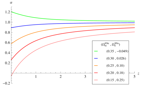
Figure 1: Smoothness parameters as functions of $z$ for the case (a)-1.

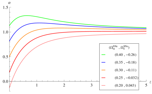
Figure 2: Smoothness parameters as functions of $z$ for the case (a)-2.

We require the smoothness parameter to be $0\leq\alpha(z)\leq 1$. In the case where this condition is not satisfied, we conclude that the tension between SNe and CMB observations cannot be resolved by only introducing the small scale inhomogeneities. The smoothness parameter satisfies the condition (11) in the following parameter region:

$$\begin{array}[]{lll}{\text{(}a)-1}&:&0.16\lesssim\Omega_{\rm m}^{\rm SNe}\leq 0.3175,\\ {\text{(}a)-2}&:&0.22\lesssim\Omega_{\rm m}^{\rm SNe}\lesssim 0.23.\end{array}$$ (22)

The smoothness parameters are monotonically increasing functions of the redshift and it asymptotically approaches to unity if the matter density parameter is included in the parameter region (22). The parameter region given by (22) is consistent with the fact that $\Omega^{\rm SNe}_{\rm m}$ tends to be smaller than $\Omega^{\rm CMB}_{\rm m}$Ade:2013zuv .

(b): $\Omega_{k}^{\rm SNe}=0$

Smoothness parameters for various $w^{\rm SNe}$ in the cases (b)-1 and 2 is shown in Figs. 3 and 4, respectively.

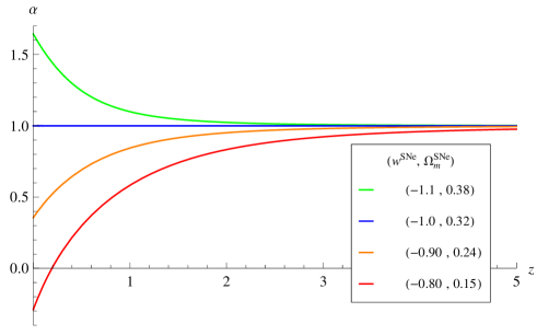
Figure 3: Smoothness parameters as functions of $z$ for the case (b)-1.

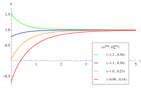
Figure 4: Smoothness parameters as functions of $z$ for the case (b)-2.

The equation of state parameter for SNe $w^{\rm SNe}$ has to satisfy the following conditions to guarantee the condition $0\leq\alpha(z)\leq 1$.

$$\begin{array}[]{lll}{\text{(}b)-1}&:&-1.0\leq w^{\rm SNe}\lesssim-0.84,\\ {\text{(}b)-2}&:&-1.13\leq w^{\rm SNe}\lesssim-1.0.\end{array}$$ (23)

The smoothness parameters monotonically increase with the redshift and asymptote to unity in the above parameter region. In both cases, $w^{\rm SNe}$ must be larger than $w^{\rm CMB}$. The results of the case (b) suggest that the equation of state parameters can differ from each other. From the result of the case (b)-1, even if dark energy is the cosmological constant, that is $w^{\rm CMB}=-1$, $w^{\rm SNe}$ can be different from unity by the effect of the small scale inhomogeneities.

V Summary and Conclusion

In this letter, we have proposed a way to obtain the information about the small scale inhomogeneities from the tension between SNe and other observations with much larger diameter sources, such as CMB. We have used the Dyer-Roeder approach to take account of the effect of the small scale inhomogeneities for distance-redshift relation of SNe. The redshift dependent smoothness parameter $\alpha(z)$ has been introduced as the fraction of the smoothly distributed matter. Because of this definition, we required $\alpha(z)$ to be $0\leq\alpha(z)\leq 1$.

We have determined the smoothness parameter as a function of the redshift so that it compensates the deviation of cosmological parameters estimated by SNe data from those estimated by CMB data. The existence of such a $\alpha(z)$ satisfying $0\leq\alpha(z)\leq 1$ implies that the small scale inhomogeneities may cause the tension between CMB and SNe observations. That is, the small scale inhomogeneities may be an origin of significant systematic error in SNe observations if we do not properly handle its effects.

We have introduced the smoothness parameter as a phenomenological parameter characterizes the small scale inhomogeneities. Therefore, the functional form of $\alpha(z)$ contains information about structure formation history of the universe. In this sence, we naturally expect that $\alpha(z)$ is monotonically increasing function of $z$ and asymptote to unity. We found that $\alpha(z)$ satisfies this property for our cases once we require $0\leq\alpha(z)\leq 1$. Our analysis implies that comparison between SNe and CMB observations may provide us the information about small scale inhomogeneities and its formation history.

It should be noted that, to make our proposal more realistic, several problems must be resolved. First, other origins of uncertainty in SNe observations, such as absorption effects and bias from poor understanding of the explorsion mechanism, must be resolved. Besides those effects, our analysis is based on the “opacity hypothesis”Fleury:2013sna which states that all observed SNe have path through the region far from clumps. Nevertheless, our proposal is unique one which has potential to probe extremely small scale ($>10^{15}$cm) inhomogeneities in cosmological observations in the future.

References

- (1) P. A. R. Ade et al. [Planck Collaboration], Astron. Astrophys. (2014) [arXiv:1303.5076 [astro-ph.CO]].
- (2) P. Fleury, H. Dupuy and J. P. Uzan, Phys. Rev. Lett. 111, 091302 (2013) [arXiv:1304.7791 [astro-ph.CO]].
- (3) P. Fleury, H. Dupuy and J. P. Uzan, Phys. Rev. D 87, no. 12, 123526 (2013) [arXiv:1302.5308 [astro-ph.CO]].
- (4) C. C. Dyer and R. C. Roeder, ApJ, 174, L115 (1972).
- (5) C. C. Dyer and R. C. Roeder, ApJ, 180, L31 (1973).
- (6) P. Fleury, JCAP 1406, 054 (2014) [arXiv:1402.3123 [astro-ph.CO]].
- (7) V. C. Busti, R. C. Santos and J. A. S. Lima, Phys. Rev. 85, 103503 (2012) [arXiv:1202.0449 [astro-ph.CO]].
- (8) E. V. Linder, A&A, 206, 190 (1988).
- (9) E. V. Linder, ApJ, 497, 28 (1998).
- (10) J. A. S. Lima, V. C. Busti and R. C. Santos, Phys. Rev. D 89, 067301 (2014) [arXiv:1301.5360 [astro-ph.CO]].
- (11) Sachs R. K., Proc. Roy. Soc. London A 264, 309 (1961).
- (12) M. Sasaki, Cosmological Gravitational Lens Equation: Its Validity And Limitation, Prog. Theor. Phys. 90 753 (1993).
- (13) Schneider, P., Ehlers, J. & Falco, E. E., Gravitational Lenses, Springer-Verlag, Berlin (1992).