Endogenous crisis waves: a stochastic model with synchronized collective behavior

Abstract

We propose a simple framework to understand commonly observed crisis waves in macroeconomic Agent Based models, that is also relevant to a variety of other physical or biological situations where synchronization occurs. We compute exactly the phase diagram of the model and the location of the synchronization transition in parameter space. Many modifications and extensions can be studied, confirming that the synchronization transition is extremely robust against various sources of noise or imperfections.

Synchronisation is arguably among the most baffling cooperative phenomenon in nature Sync . Examples abound in physics and chemistry, but biological realizations are probably the most relevant to us as they involve in particular the synchronization of pacemaker cells in the heart or of neurons firing in the brain. Synchronization of clapping in concert halls or of flashing in assemblies of thousands of fireflies are also well known. The latter case is particularly interesting: although the effect is so to say visible to the naked eye, its very existence is so counter-intuitive that for several decades no one could come up with a plausible theory. As vividly recounted by Strogatz Sync , scientists swayed between denial (assigning the flashing to a periodic quiver of the eyelids of the observer, or to the unavoidable presence of a “maestro”) and explanations that were “more remarkable than the phenomenon itself” Sync . The idea that interacting oscillators can generically synchronize only slowly emerged at the end of the sixties Winfree , before becoming a well-established mathematical truth with the work of Kuramoto Kuramoto , Strogatz & collaborators Strogatz , and many others (for a review, see Ritort ).

Still, the phenomenon is so unexpected (at least for those only vaguely acquainted with these results) that while working on a stylized agent based model (ABM) of the macroeconomy Gualdi , we first disbelieved our results. We found a whole region of parameter space where the dynamics appeared to be (see Fig. 1) a nearly periodic succession of eras of prosperity interrupted by acute crisis of purely endogenous origin – indeed, no adverse exogenous shocks are present in our model; for details, see Gualdi . In view of the amount of heterogeneity and randomness in our model (firms in our economy are all different, bankrupted firms are revived at Poisson random times, etc.), such a regular succession of crises waves is both interesting and surprising, and begs for a convincing theoretical explanation. However, although highly stylized, our ABM is too complex to be amenable to an exact analytical treatment, so further simplification is needed. This led us to the bare-bones model described below, which indeed exhibits – in fact, to our surprise – a synchronization transition. This model can be analyzed using reasonably straightforward mathematical tools. For instance the location of the transition in parameter space can be computed exactly. Many modifications and extensions of the model can be studied, exactly or numerically. Their analysis confirms that the synchronization transition is extremely robust, in particular against various sources of noise and imperfections.

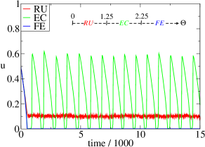
Figure 1: Typical trajectories of the unemployment rate $u$ as a function of time for the macroeconomic agent based model described in Gualdi , for different bankruptcy thresholds $\Theta$. As $\Theta$ is increased, the economy evolves from a phase of residual unemployment (RU), endogenous crises (EC) and finally full employment (FE). In the EC phase, surprisingly, one observes nearly periodic bursts of unemployment, corresponding to collective waves of bankruptcies.

Our model is an alternative to the well-known Kuramoto model that has been studied inside-out Kuramoto ; Strogatz ; Ritort , and which starts from the assumption that isolated individual elements are oscillators. Our setting is directly motivated from the macroeconomic model we wanted to elucidate, and is in fact close in spirit to “integrate-and-fire” models of neurons Strogatz . It can also be rephrased as a mean-field model for epidemic dynamics Epidemic , fiber bundles Hansen , depinning of elastic manifolds Depinning , or interbank default contagion Battiston . In order to describe the model, we choose to keep with the vocabulary of our macroeconomic model – transposition to other contexts is quite transparent and will be discussed below. Each firm $i=1,\dots,N$ is characterized by its “financial fragility” measured by the ratio $x_{i}$ of its outstanding debt to total assets. We use the convention that $x_{i}<0$ for indebted firms, and $x_{i}>0$ for cash/loan-rich firms. In the course of time, this ratio can increase or decrease due to the success of its business, its needs for cash, etc. We posit Gualdi that when the financial fragility exceeds a certain threshold $\Theta$ (i.e. when $x_{i}\leq-\Theta$) banks are reluctant to restructure the debt of the firm, which then files for bankruptcy. (In a first version of the model, we assume this occurs with probability $1$ as soon as $x_{i}\leq-\Theta$, but one can also consider the case where bankruptcy is not certain and happens with probability $\kappa\mathds{1}_{x_{i}\leq-\Theta}$ per unit time, see below). Until firms hit the threshold, the evolution of $x_{i}$ is modeled as a biased random walk. The most important feature of the model is the feedback between bankruptcies and the drift of these random walks. In the absence of money creation (i.e. if the banking sector does not act as a buffer), the outstanding debt of the defaulted firm is spread between remaining firms – thereby directly increasing their financial fragility – and the household sector, leading to a decrease of its purchasing power and hence worsened business conditions for the surviving firms (see Gualdi for a concrete implementation of this general idea). In both cases, this gives a negative contribution to the drift of $x_{i}$’s. Finally, bankrupted firms are either revived or replaced by new firms at a certain rate $\varphi$ per unit time, and start with a zero initial fragility.

Taking the limit of a large number of firms, the above rules translate into the following Fokker-Planck equation for the probability density $P(x,t)$ of observing firms with a certain fragility between $x$ and $x+{\rm d}x$ at time $t$:

$$\dot{P}(x,t)=DP^{\prime\prime}(x,t)+b(t)P^{\prime}(x,t)+J(t)\delta(x-\Theta),$$ (1)

where we made a translation $x\to x+\Theta$, $\phi(t)=\int_{0}^{\infty}{\rm d}xP(x,t)$ is the fraction of active firms at time $t$, $J(t)$ is the flux of new-born firms at time $t$. The boundary condition $P(0,t)=0,\forall t$ corresponds to case where bankruptcy is immediate, as soon as the threshold is reached, and

$$b(t)=b+\beta DP^{\prime}(0,t)\Theta\,$$ (2)

is the drift, that itself depends on the flux of bankruptcies $DP^{\prime}(0,t)$ (i.e. the number of firms that cross $x=0$ at time $t$ that spread an extra debt $\Theta$) through a phenomenological, adimensional parameter $\beta$ that measures the strength of the feedback. Note that with our sign convention, a positive $b(t)$ corresponds to a drift towards more negative values of $x$. The reinjection current $J(t)$ is either (model I) a time-independent constant $J(t)=\varphi$, modeling the fact that new firms are created at a constant rate, independently of the number of existing firms, or (model II) given by $J(t)=(1-\phi(t))\varphi$, meaning that bankrupted firms have a probability $\varphi$ per unit time to be revived, in line with the choice made in the macroeconomic model studied in Gualdi .

In both cases the model contains 5 parameters: $D,b,\varphi,\Theta$ and the feedback parameter $\beta$, but two can be fixed by the choice of units of time $t$ and “length” $x$. This leaves us with three adimensional parameters: $\beta$, the Peclet number $Pe=b\Theta/D$ that compares drift to diffusion and $z=b/(\Theta\varphi)$ that compares the average revival time to the time needed to travel $\Theta$ under the action of the drift $b$. $Pe\gg 1$ means that diffusion is a small correction to drift in typical trajectories, whereas $z\ll 1$ means that revival is fast compared to the time to bankruptcy due to drift only. As implicitly assumed in the above discussion, we will only consider the case $b>0$ (i.e. a negative drift on $x$), that allows the existence of a stationary state in the absence of feedback ($\beta=0$). This also describes the economy considered in Gualdi : for non storable goods and in the absence of productivity gains or innovation, our myopic firms have a tendency to over-produce and lose money on average.

We therefore look for a stationary state $P_{0}(x)$, characterized by a constant bankruptcy flux $J(t)=J_{0}$ and constant $\phi(t)=\phi_{0}$. Because $DP_{0}^{\prime}(x=0)$ is the out-coming flux, and the fraction of active firms $\phi$ is time independent, it follows that $DP_{0}^{\prime}(x=0)=J_{0}$ and this leads to a constant drift $b_{0}=b+\beta\Theta J_{0}$. By setting $\dot{P}\equiv 0$ in Eq. (1), it is easy to show that:

$$P_{0}(x)=\frac{J_{0}}{b_{0}}\times\begin{cases}(1-e^{-\hat{x}})&\text{for }\hat{x}<\hat{\Theta}\ ,\\ (e^{\hat{\Theta}}-1)e^{-\hat{x}}&\text{for }\hat{x}>\hat{\Theta}\ ,\\ \end{cases}$$ (3)

where $\hat{x}=b_{0}x/D$ and $\hat{\Theta}=b_{0}\Theta/D$ are adimensional “lengths”. The stationary solution for $P_{0}(x)$ is therefore given in terms of the unknown parameters $J_{0},\phi_{0}$ and $b_{0}$ that are determined from:

$$\phi_{0}\equiv\int_{0}^{\infty}dxP_{0}(x)=\frac{J_{0}\Theta}{b_{0}};\qquad b_{0}=b+\beta J_{0}\Theta.$$ (4)

For model I, one has $J_{0}=\varphi$ and $\phi_{0}$ and $b_{0}$ are immediately obtained. For model II, $J_{0}=(1-\phi_{0})\varphi$ gives a third equation. Using Eqs. (4), we can solve for $b_{0}=\frac{b}{1-\beta\phi_{0}}$ and $J_{0}=\frac{\phi_{0}}{\Theta}\frac{b}{1-\beta\phi_{0}}$ and obtain a self-consistent equation

$$\frac{\phi_{0}}{\Theta}\frac{b}{1-\beta\phi_{0}}=(1-\phi_{0})\varphi\ ,$$ (5)

which leads to a second degree equation for $\phi_{0}$. If the time needed for revival is much shorter than the lifetime of the firms, $z\to 0$, we expect that $\phi_{0}\to 1$, at least for small $\beta$’s. This allows one to choose the correct sign of the solution:

$$\phi_{0}=\frac{1}{2\beta}\left[1+\beta+z-\sqrt{z^{2}+2z(1+\beta)+(1-\beta)^{2}}\right]\ .$$ (6)

It can easily be checked that this solution is then always such that $\phi_{0}\in[0,\min(1,1/\beta)]$. Therefore, the stationary solution always exists, and $b_{0}$ never diverges, which would be an obvious sign of an instability (see below for a case where this divergence actually happens). Still, the question is whether this stationary solution is dynamically stable. We therefore write:

$$P(x,t)=P_{0}(x)+\epsilon P_{1}(x,t),$$ (7)

which induces corresponding $O(\epsilon)$ corrections to $\phi(t)=\phi_{0}+\epsilon\phi_{1}(t)$ and similarly for $J(t)$ and $b(t)$. To order $\epsilon$, the diffusion equation for $P$ becomes, both for models I and II:

$$[G^{-1}P_{1}](x,t) \equiv \dot{P}_{1}(x,t)-DP_{1}^{\prime\prime}(x,t)-b_{0}P_{1}^{\prime}(x,t)$$ (8)

$$= b_{1}(t)P_{0}^{\prime}(x)-\varphi\phi_{1}(t)\delta(x-\Theta)\,$$

where $G$ is the propagator of random walks with a wall at $x=0$ and drift $b_{0}$, given by the method of images Redner :

$$G(x,t|y,t-\tau) = \frac{1}{\sqrt{4\pi D\tau}}\left\{\exp\left[-\frac{(x-y+b_{0}\tau)^{2}}{4D\tau}\right]\right.$$ (9)

$$- \left.e^{b_{0}y/D}\exp\left[-\frac{(x+y+b_{0}\tau)^{2}}{4D\tau}\right]\right\}$$

Therefore, formally:

$$\begin{split}P_{1}(x,t)&=\int_{0}^{\infty}d\tau\int_{0}^{\infty}dyG(x,t|y,t-\tau)\\ &\times\left[b_{1}(t-\tau)P_{0}^{\prime}(y)-\varphi\phi_{1}(t-\tau)\delta(y-\Theta)\right].\end{split}$$ (10)

This expression gives $P_{1}(x,t)$ in terms of $b_{1}(t)$ and $\phi_{1}(t)$. Using the definition of $b(t)$ and $\phi(t)$ then leads to self-consistent dynamical equations for $b_{1}(t)$ and $\phi_{1}(t)$, which are slightly different in models I and II. We focus on model II and we assume (and check self-consistently) that $\phi_{1}(t)=\Phi e^{\alpha t}$ and $b_{1}(t)=B\Theta e^{\alpha t}$, where $\alpha$ is (a priori) a complex number with $b_{0}^{2}+4D{\rm Re}\,(\alpha)\geq 0$ to have convergent integrals. After simple algebra, one finally finds that $B$ and $\Phi$ have to obey the following equations:

$$\Phi = -\frac{B\phi_{0}}{\alpha}\frac{1-e^{K\Theta}}{1-KD/b_{0}}-\varphi\Phi\frac{1-e^{K\Theta}}{\alpha};$$

$$B = -\beta\varphi\Phi e^{K\Theta}+B\beta\phi_{0}\frac{1-e^{K\Theta}}{1-KD/b_{0}}\ ,$$ (11)

where $K=\frac{b_{0}}{2D}\left(1-\sqrt{1+\frac{4\alpha D}{b_{0}^{2}}}\right)$. These have non-zero solution only if $\alpha$ satisfies the equation footnote :

$$\beta\phi_{0}(\alpha+\varphi)=[\alpha+\varphi(1-e^{K\Theta})]\frac{1-KD/b_{0}}{1-e^{K\Theta}}\ .$$ (12)

This equation has to be solved numerically in the complex plane, and one has to choose the solution with the largest ${\rm Re}\,(\alpha)$ that dominates the long-time evolution. We find three different possibilities: ${\rm Re}\,(\alpha)<0,{\rm Im}\,(\alpha)=0$: the stationary state $P_{0}$ is linearly stable and relaxation towards it is exponential; ${\rm Re}\,(\alpha)<0,{\rm Im}\,(\alpha)\neq 0$: the stationary state $P_{0}$ is linearly stable and relaxation towards it is exponential with oscillations; ${\rm Re}\,(\alpha)>0,{\rm Im}\,(\alpha)\neq 0$: $P_{0}$ is linearly unstable and the oscillations are the precursor of the synchronized state observed numerically. An example of the dependence of $\alpha$ as a function of $\varphi$ for fixed $\beta$ and $z$ is given in Fig. 2-a. One sees that ${\rm Re}\,(\alpha)$ crosses zero continuously for a critical value $\varphi_{c}$, for which ${\rm Im}\,(\alpha)\neq 0$. The corresponding evolution of fraction of inactive firms, $1-\phi(t)$, is given in Fig. 2-b, where we show a numerical integration of the Fokker-Planck equation, Eq. (1), but identical results are obtained from a random walk simulation of $10^{5}$ firms obeying the same dynamics. One clearly sees that the synchronized behavior sets in exactly at the value $\varphi=\varphi_{c}\approx 35.15$ (for $\beta=1.3$ and $z=0.002$) predicted by the linear stability analysis. The transition is found to be continuous, with an amplitude of the oscillations that vanishes at the transition, and a frequency given by ${\rm Im}\,(\alpha_{c})$. The phase diagrams in the $(Pe,\beta)$ plane (for a fixed $z$) and in the $(z,\beta)$ plane (for a fixed $Pe$) are given in Fig. 3. The conclusion of our analysis is that crises waves and synchronization indeed appear in our skeleton macroeconomic model. What is quite non trivial is that this transition survives the fact that firms perform independent Brownian motion and are reinjected in the system at random Poisson time. Similar conclusions of course hold for the Kuramoto model as well.

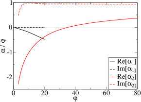
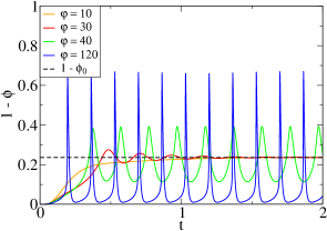
Figure 2: (Top) Numerical solutions of Eq. (12): for small values of $\varphi$ there is only one linearly stable solution without oscillations ($\alpha_{1}$); for intermediate values of $\varphi$ a second linearly stable solution appears with oscillations ($\alpha_{2}$); for high values of $\varphi$ there is only a linearly unstable solution with oscillations corresponding to the appearance of the synchronized behavior. (Bottom) Typical trajectories of the fraction of bankrupt firms $1-\phi$ as a function of time for different values of $\varphi$. $\phi_{0}$ is the theoretical value of stationary fraction of active firms, given by Eq. (6). For $\varphi>\varphi_{c}$ the synchronized behavior settles in. The plot corresponds to $z=0.002$ and $\beta=1.3$.

The above stability analysis can be extended in different directions. First, the reinjection flux can be taken as a constant $J_{0}=\varphi$ (Model I), leading to an even more unstable system (see footnote ). Second, the reinjection flux does not need to be localized on $x=\Theta$ but it can be spread out over a certain region, i.e. one can replace the term $J(t)\delta(x-\Theta)$ in Eq. (1) by $J(t)f(x-\Theta)$, where $f(x)$ is a function peaked in zero, normalized to one, and with finite width $w$, with only quantitative changes. In fact, starting with a $\delta$ function in the synchronized phase, one can induce the transition by increasing the width $w$ beyond some critical value $w_{c}$. Third, one can replace the deterministic bankruptcy condition by a stochastic one, by adding a term $-\kappa\theta(-x)$ to the Fokker-Planck equation and setting $b(t)=b+\beta\kappa\int_{-\infty}^{0}\mathrm{d}x(\Theta-x)P(x,t)$. The above case corresponds to the limit $\kappa=\infty$. One finds that the synchronization phenomenon survives at finite $\kappa$. For example, when $\beta=1.3,z=0.002,\varphi=80$, synchronization occurs for $\kappa>\kappa_{c}\approx 100$. It is important (but again not very intuitive) that the synchronization phenomenon does not sensitively depend on the presence of a well defined threshold – one does not expect neurons or fireflies to be perfectly tuned to a precise firing threshold. Finally, we have investigated the case where the bankruptcy feedback depends on the number of active firms, i.e. $b(t)=b+\frac{\beta}{\phi(t)}DP^{\prime}(0,t)\Theta$, corresponding to the case where the debt of the failing firms is spread among the surviving firms only. In this case, we find that the above stationary state $P_{0}(x)$ ceases to exist as soon as $\beta>1$, which becomes the threshold for synchronized behavior. In this case, the transition is found to be first order.

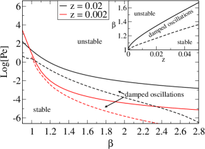
Figure 3: Phase diagram of the model in Eq. (1) in the $(\beta,Pe)$ plane as given by the solutions of Eq. (12) with $z=0.02$ (black lines) and $z=0.002$ (red lines). Dashed lines separate the region where the maximal solution has ${\rm Re}\,(\alpha)<0$ and ${\rm Im}\,(\alpha)=0$ (stable) from the region where ${\rm Re}\,(\alpha)<0$ and ${\rm Im}\,(\alpha)\neq 0$ (damped oscillations). Full lines separate the latter region from the one where ${\rm Re}\,(\alpha)>0$ (unstable). In the inset we plot the phase diagram in the $(\beta,z)$ for $Pe=0.5$.

Finally, we want to mention different potentially interesting interpretations of our model. First, interbank default contagion, which has become a major theme since the 2008 crisis Battiston . Here, the translation is almost immediate: since the assets of one bank is the liability of another, the default of one bank reduces the equity of its lenders, therefore pushing themselves closer to default. Treating the model in mean-field immediately leads to a Fokker-Planck equation like Eq.(1). In a recent study of a similar model, J. Bonart Bonart has shown that the default rate can diverge after a finite time, yet another signal of the collective synchronization effects studied here. Second, one can consider an epidemic model Epidemic where $x_{i}$ gauges the level of infection of individual $i$. When $x_{i}>\Theta$, the illness declares itself and the disease becomes strongly contagious. The flux $J(t)$ would then model non-infected new immigrants in the population. The model then predicts the possibility of sporadic outbreaks of the epidemics. Yet another interpretation of our model is in terms of the fiber bundle model for fracture Hansen , allowing for “self-healing”, i.e. the possibility for broken links to reform in time. Finally, one can interpret Eq. (1) as a mean-field description of the depinning transition Depinning , where each particle $i$ is subject to an increasing force $f_{i}=x_{i}$ until $f_{i}$ reaches a local depinning threshold $\Theta$. At this point, the particle advances and thereby relaxes the force acting on it, and gets trapped again. However, if one assumes that particle $i$ is elastically coupled to its neighbours $j$, the forces $f_{j}$ will increase as particle $i$ depins. In mean-field, we once again end up with Eq.(1), which predicts a transition from a smooth overall progression when the external drive (here modeled by the drift $b$) is large enough to a jerky stick-slip motion for small drive. An interesting generalization is to consider that the feedback does not affect the drift $b$, as above, but the diffusion constant $D$, much as in Hebraud . This could be relevant for soft glassy matter or granular materials, where a localized yield event is often supposed to act as an effective temperature for the rest of the system. This, and other extensions, are left for future investigations.

Acknowledgements We thank J. Bonart, E. Bouchaud and J. Donier for very insightful conversations. This work was partially financed by the EU “CRISIS” project (grant number: FP7-ICT-2011-7-288501-CRISIS)

References

- (1) S. H. Strogatz, SYNC: the Emerging Science of Spontanenous Order, Hyperion, New York (2003).
- (2) A. T. Winfree, J. Theor. Biol. 16, 15 (1967).
- (3) Y. Kuramoto, Chemical Oscillations, Waves and Turbulence, Springer, New York (1984).
- (4) S. H. Strogatz, Physica D 143, 1 (2000), and refs. therein.
- (5) for a recent review, see: J. A. Acebrón, L. L. Bonilla, C. J. Pérez Vicente, F. Ritort, R. Spigleri, Reviews of Modern Physics, 77, 139 (2005), and the extensive list of references therein.
- (6) S. Gualdi, M. Tarzia, F. Zamponi, J.-P. Bouchaud, Journal of Economic Dynamics and Control (2014), http://dx.doi.org/10.1016/j.jedc.2014.08.003i
- (7) for a recent review, see: R. Pastor-Satorras, C. Castellano, P. Van Mieghem, A. Vespignani, arXiv:1408.2701v1.
- (8) for a recent review, see: S. Pradhan, A. Hansen, B. Chakrabarti, Rev. Mod. Phys. 82, 499 (2010).
- (9) D. S. Fisher, Physics Reports, 301, 113 (1998).
- (10) see e.g. J. Lorenz, S. Battiston, F. Schweitzer, Eur. Phys. J. B 71, 441 (2009).
- (11) S. Redner, A guide to first passage time problems, Cambridge University Press (2001).
- (12) For model I, the final equation is even simpler and reads: .
- (13) J. Bonart, private communication and in preparation.
- (14) P. Hébraud and F. Lequeux, Phys. Rev. Lett. 81, 2934 (1998).