Spatial Throughput Maximization of Wireless Powered Communication Networks

Abstract

Wireless charging is a promising way to power wireless nodes’ transmissions. This paper considers new dual-function access points (APs) which are able to support the energy/information transmission to/from wireless nodes. We focus on a large-scale wireless powered communication network (WPCN), and use stochastic geometry to analyze the wireless nodes’ performance tradeoff between energy harvesting and information transmission. We study two cases with battery-free and battery-deployed wireless nodes. For both cases, we consider a harvest-then-transmit protocol by partitioning each time frame into a downlink (DL) phase for energy transfer, and an uplink (UL) phase for information transfer. By jointly optimizing frame partition between the two phases and the wireless nodes’ transmit power, we maximize the wireless nodes’ spatial throughput subject to a successful information transmission probability constraint. For the battery-free case, we show that the wireless nodes prefer to choose small transmit power to obtain large transmission opportunity. For the battery-deployed case, we first study an ideal infinite-capacity battery scenario for wireless nodes, and show that the optimal charging design is not unique, due to the sufficient energy stored in the battery. We then extend to the practical finite-capacity battery scenario. Although the exact performance is difficult to be obtained analytically, it is shown to be upper and lower bounded by those in the infinite-capacity battery scenario and the battery-free case, respectively. Finally, we provide numerical results to corroborate our study.

I Introduction

By enabling the wireless devices to scavenge energy from the environment, energy harvesting has become a promising solution to provide perpetual lifetime for energy-constrained wireless networks (e.g., the wireless sensor networks) [1]. In particular, with the ability to cater to the mobility of the wireless nodes, the ambient radio-frequency (RF) signals have been considered as a vital and widely available energy resource to power wireless communication networks [2]. In recent point-to-point energy transfer experiments [3], wireless power of 3.5mW and 1uW have been harvested from the RF signals at distances of 0.6 and 11 meters, respectively. Moreover, in the experiment-based study in [4], the harvested energy from multiple energy transmitting sources is shown to be additive, which can be exploited to extend the operation range of wireless charging. Due to the appealing features of the RF-based energy harvesting, the wireless powered communication network (WPCN) [5], in which the wireless nodes exploit the harvested RF energy to power their information transmissions, has attracted growing attentions.

Different from traditional wireless networks, where the wireless nodes can draw energy from reliable power supplies (e.g., by connecting to the power grid or a battery), due to the wireless fading channels, the random movement of the wireless nodes, as well as the employed energy harvesting techniques, the amount of energy that can be harvested in a WPCN is generally uncertain. As a result, to meet the quality-of-service (QoS) requirement of the information transmission, the designed transmission schemes must be adaptive to the dynamics of the harvested RF energy. Although challenging, by assuming completely or partially known knowledge of the energy arrival processes, effective transmission schemes have been proposed in, e.g., [6]-[8]. However, the adopted energy arrival models in the above studies do not apply to the RF-based energy harvesting scenario.

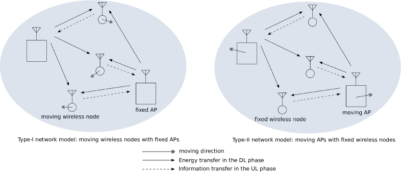
Figure 1: Two types of WPCN models with DL energy harvesting and UL information transmission.

There has been a growing research interest focusing on a point-to-point or point-to-multipoint RF energy harvesting system, where a single transmitter transmits energy to a single wireless node or multiple wireless nodes, respectively (e.g., in [5], [9], and [10]). In particular, in [5] the authors studied a point-to-multipoint system, where the energy transfer from an access point (AP) to multiple wireless nodes is separated from the information transfer from each of the wireless nodes to the AP in time domain. By exploiting the harvested energy at each wireless node, [5] investigated the optimal time allocation for energy transfer and information transfer, so as to maximize the system throughput with fairness consideration. Moreover, since the RF signals may also carry information besides energy, simultaneous wireless information and power transfer (SWIPT) has been studied in the literature (see e.g. [9], [10]), where more sophisticated receiver design is involved. In addition, we also noticed there are some works focusing on energy-efficient design for other applications (e.g., [11]-[13]).

However, most of the existing work, including the above mentioned ones, did not consider optimal transmission scheme design in a large-scale WPCN with a very large number of wireless nodes, mainly due to the following reasons: 1) it is difficult to design a scalable transmission scheme that can be efficiently implemented with the increasing number of wireless nodes; and 2) due to the wireless fading channels as well as the random placement of both energy transmitters and wireless nodes, it is challenging to analytically characterize the harvested RF energy by a wireless node from multiple energy transmitters. It came to our attention that stochastic geometry, as a novel way to analyze large-scale communication networks, provides a set of powerful mathematical tools for modeling and designing the wireless networks [14]. Moreover, the mathematical tools (e.g., probability generating functional (PGFL) of a Poisson point process (PPP)), which facilitate the interference analysis in a wireless communication network [15], can also help characterize the harvested RF energy in a WPCN [16], [17].

In this paper, by using tools from stochastic geometry, we aim at optimizing bidirectional energy harvesting and information transmission in a large-scale WPCN. We consider a new type of dual-function APs which are able to coordinate energy/information transfer to/from the wireless nodes. We also consider two types of networks models. As illustrated in Fig. 1, in Type-I network model, the wireless nodes (e.g., the portable electronic devices or the unmanned vehicles [18]) are assumed to independently move in the system over frames, while the locations of the APs are fixed. In Type-II network model, however, the APs (e.g., the wireless charging vehicles [19]) are assumed to independently move in the system over frames, while the locations of the wireless nodes are fixed. We show that the wireless node’s downlink (DL) energy harvesting performance and the uplink (UL) information transfer performance can be identically characterized for both types of network models. Moreover, depending on whether each wireless node deploys a rechargeable battery, we consider two cases with battery-free and battery-deployed wireless nodes, respectively, and study the effects of battery storage. For both cases, we maximize the spatial throughput of the wireless nodes, which is defined as the total throughput that is achieved by the wireless nodes per unit network area averaged over all information transmission phases (bps/Hz/unit-area) [20].

The key contributions of this paper are summarized as follows.

• Novel harvest-then-transmit protocol to power a large-scale network: In Section II, we propose a new harvest-then-transmit protocol by extending that in [5], where each time frame is partitioned into a DL phase for energy transfer from the APs to the wireless nodes, and an UL phase for information transfer from each wireless node to its associated AP. We show that the proposed harvest-then-transmit protocol is scalable and thus can be efficiently implemented in a large-scale network.

• Problem formulation and simplification for spatial throughput maximization: In Section III, by jointly optimizing time frame partition between the DL and UL phases and the wireless nodes’ transmit power, we formulate the spatial throughput maximization problem under a successful information transmission probability constraint. To make the problem analytically tractable, we simplify the problem by utilizing the equivalence of the successful information transmission probability constraint to a transmission probability constraint plus a minimum transmit power constraint.

• Spatial throughput maximization for battery-free wireless nodes: In Section IV, we solve the spatial throughput maximization problem in the battery-free case, by studying the effects of the AP density and the wireless node density. We also show that at the optimality the wireless nodes generally prefer to select a small transmit power, for obtaining large transmission opportunity.

• Spatial throughput maximization for battery-deployed wireless nodes: In Section V, we first study an ideal infinite-capacity battery scenario, and show that all the feasible time frame partition and UL transmit power are optimal, since energy stored in the battery is sufficient over time. We then extend our study to the practical finite-capacity battery scenario. By proposing a new tight lower bound for the transmission probability, we approximately solve the spatial throughput maximization problem.

We note only limited studies in [16], [17], [21], and [22] have adopted stochastic geometry to study the large-scale communication networks enabled by energy harvesting. Different from these existing studies, we consider the WPCN where dual functional APs transmit energy and receive information to/from wireless nodes. Moreover, we focus on characterizing optimal tradeoffs between the DL energy transfer and the UL information transfer, for both battery-free and battery-deployed cases, and theoretically analyze the impact of battery storage on the network throughput performance. In addition, different from most existing studies based on stochastic geometry that only focused on average system performance of one snapshot, in this paper, we pursue a long-term average system analysis, and successfully obtain tractable system performance in both DL and UL.

II System Model

We consider a WPCN with stochastically deployed APs and wireless nodes, where each wireless node harvests energy broadcast by the APs, and then uses the harvested energy to support its information transmission to the associated AP. As shown in Fig. 1, we assume either the wireless nodes or the APs move in the system. In this section, we first present the detailed operations at each wireless node for both battery-free and battery-deployed cases, and then develop the network model based on stochastic geometry.

II-A System Operation Model

We consider that each AP has reliable power supply (e.g., by connecting to the power grid or equipping with large-capacity battery storage in Type-I or Type-II network model, respectively), while each wireless node is not equipped with any embedded energy sources but an RF energy harvesting device. Thus, the wireless nodes are able to harvest the energy broadcast by the APs, and use them to support their information transmissions to the APs. Similar to the practical radio frequency identification (RFID) system that coexists with the reader network over the same frequency (around 915MHz) [23], we assume all the APs and wireless nodes operate over the same frequency band. We also assume all the APs and wireless nodes are each equipped with a single antenna, as in the case of the wireless sensor networks. We partition energy transfer and information transfer in time domain, as shown in Fig. 2. We assume the network is frame-based in time and consider a harvest-then-transmit protocol for the wireless nodes. Specifically, we assume each frame consists of $T>1$ slots, indexing from $0$ to $T-1$, and all the slots are synchronized among APs and wireless nodes. In each frame, we assign slot $0$ to slot $N-1$, $1\leq N\leq T-1$, to the APs for broadcasting energy in the DL phase, and assign the remaining slots, i.e., slot $N$ to slot $T-1$, to the wireless nodes for transmitting information in the UL phase. We denote the transmit power of the APs and the wireless nodes as $P_{D}>0$ and $P_{U}>0$, respectively. We assume $0<P_{U}\leq P_{\max}$, where $P_{\max}$ is the maximum allowable transmit power of each wireless node. It is worth noting that to design a scalable transmission scheme for a large-scale WPCN (e.g., wireless sensor or RFID networks), where the wireless nodes usually operate at low transmit power, we consider the same $P_{U}$ and $N$ for each wireless node, and optimize $P_{U}$ and $N$ globally for a homogeneous stochastic network as will be shown later. Thus, wireless nodes do not need to communicate and coordinate in interference management, which is easy to implement in practice. Moreover, due to the wireless fading channels as well as the low energy harvesting efficiency of today’s RFID technology [24], the amount of energy that can be collected in one slot is usually small, and is difficult to be effectively exploited by the wireless nodes. As a result, as in the practical energy harvesting devices, e.g., the P2110 power harvester receiver [25] designed by the Powercast corporation, we consider that a small-sized capacitor is integrated in the circuits of the energy harvesting device, based on which, the harvested energy from slot $0$ to slot $N-1$ in the DL phase can be accumulated without the usage of additional battery, and then entirely boosted out for exploitation by each wireless node (for UL transmission or battery charging), as shown in Fig. 2. For each wireless node $i$, denote $Z_{F,i}(t)$ as the amount of energy harvested in DL slot $t$ of frame $F$, $0\leq t\leq N-1$, $1\leq F\leq\infty$, and $Z_{F,i}$ as the total amount of energy harvested in the DL phase of frame $F$. We have $Z_{F,i}=\sum_{t=0}^{N-1}Z_{F,i}(t)$.

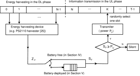
Figure 2: Energy harvesting and information transmission for each wireless node in each frame.

We denote $S_{F,i}$ as the amount of energy that is available to wireless node $i$ at the beginning of the UL phase of frame $F$. In the following, depending on whether a wireless node is equipped with a rechargeable battery (or any other energy storage devices) to store the total harvested DL energy $Z_{F,i}$ in each frame $F$, we consider two cases with battery-free and battery-deployed wireless nodes, respectively. In each case, by applying a $P_{U}$-threshold based UL transmission decision as in the literature (e.g., [16], [17], and [21]), we model the evolvement of $S_{F,i}$ over $F$. For convenience, we assume a normalized unit slot time in the sequel without loss of generality, and thus we can use the terms of energy and power interchangeably.

II-A1 Battery-free Case

As show in Fig. 2, in each frame $F$, due to the lack of energy storage, the wireless nodes manage the harvested energy in a myopic manner, i.e., all the harvested energy $Z_{F,i}$ is consumed within the current frame $F$. Moreover, if $Z_{F,i}\geq P_{U}$, wireless node $i$ decides to transmit information with power $P_{U}$ in the UL phase; otherwise, it stays silent in the UL phase of frame $F$. Since the unused amount of energy in the current frame (i.e., $Z_{F,i}-P_{U}$, if $Z_{F,i}\geq P_{U}$, or $Z_{F,i}$, otherwise) will not be kept for future use, for any $F\in\{1,...,\infty\}$, we can easily obtain

$$S_{F,i}=Z_{F,i}.$$ (1)

II-A2 Battery-deployed Case

Unlike the battery-free case, by deploying a rechargeable battery in the device circuit, the wireless nodes can store the unused energy in the current frame for future use, as long as the battery capacity allows. Thus, the harvested energy can be exploited more effectively in the battery-deployed case than that in the battery-free case in general. As shown in Fig. 2, in each frame $F$, if the battery level at the beginning of the UL phase, given by $S_{F,i}$, is no smaller than the required UL transmit power $P_{U}$, the wireless node decides to transmit in the UL; otherwise, it stays silent in the UL phase. Let the battery capacity be $C$ with $P_{U}\leq C\leq\infty$. For any $F\in\{1,...,\infty\}$, given $S_{F-1,i}$, by subtracting the consumed energy in the UL phase of frame $F-1$ and adding the harvested energy in the DL phase of frame $F$, we obtain $S_{F,i}$ as

$$S_{F,i}=\min(S_{F-1,i}-P_{U}I(S_{F-1,i}\geq P_{U})+Z_{F,i},C),$$ (2)

where $S_{0,i}=0$ and the indicator function $I(x)=1$ if $x$ is true, and $I(x)=0$ otherwise. Note that $C=\infty$ is an ideal scenario with infinite-capacity battery. It is easy to find that in this scenario, for any $F\in\{1,...,\infty\}$, (2) is reduced to

$$S_{F,i}=S_{F-1,i}-P_{U}I(S_{F-1,i}\geq P_{U})+Z_{F,i}.$$ (3)

At last, in the UL transmission, for both cases with battery-free and battery-deployed wireless nodes, we assume there is no transmission coordination between the wireless nodes for simplicity, as in [22]. We thus adopt independent transmission scheduling for the wireless nodes. Specifically, to reduce the potentially high interference level in the UL due to the independent transmissions of the wireless nodes, we assume that if a wireless node $i$ decides to transmit, it randomly selects a slot from slot $N$ to slot $T-1$ in the UL phase with equal probability of $1/(T-N)$, and transmits its information in this slot with transmit power $P_{U}$ to its nearest AP, as in [16] and [27], for achieving good communication quality. The UL information transmission is successful if the received signal-to-interference-plus-noise-ratio (SINR) at the AP is no smaller than a target SINR threshold, denoted by $\beta>0$.

II-B Network Model

Based on the operations of the wireless nodes and the APs, in this subsection, we develop the network model based on stochastic geometry, and then characterize the harvested energy of the wireless node in each frame.

As shown in Fig. 1, we consider two types of network models, which are Type-I network model, with moving wireless nodes and static APs, and Type-II network model, with moving APs and static wireless nodes. In both types of networks models, we assume the wireless nodes and the APs are initialized as two independent homogeneous PPPs, denoted by $\Phi(\lambda_{w})$, of wireless node density $\lambda_{w}>0$, and $\Phi(\lambda_{AP})$, of AP density $\lambda_{AP}>0$, respectively. In Type-I network model, we assume all the APs stay at their initialized locations in all frames, while the wireless nodes independently change their locations in each frame based on the random walk model considered in [28]. Specifically, at the beginning of each frame, each wireless node is independently displaced from its previous location in the proceeding frame to a new location in the current frame; and stays at its new location within the current frame. According to the Displacement Theorem in [28], the homogeneous PPP $\Phi(\lambda_{w})$ is preserved by the independently displaced wireless nodes in each frame. Similarly, in Type-II network model, we assume the wireless nodes stay at their initialized locations in all frames, while the APs are independently displaced over frames as the wireless nodes in Type-I network model. Clearly, the homogeneous PPP $\Phi(\lambda_{AP})$ is also preserved by the independently displaced APs in each frame in Type-II network model.

Let $\Phi(\lambda_{AP})=\{X\}$ and $\Phi(\lambda_{w})=\{Y\}$, where $X,Y\in\mathbb{R}^{2}$ denote the coordinates of the APs and wireless nodes, respectively. As in the existing literature that studied wireless charging based on stochastic geometry (e.g., [17], [21], and [22]), we assume Rayleigh flat fading channels with path-loss. We also assume the Rayleigh fading channels vary independently over different time slots. In each slot $t$ of a particular frame, the radio signal transmitted by an AP/wireless node is received at the origin with strength $|X|^{-\alpha}h_{X}(t)$ and $|Y|^{-\alpha}h_{Y}(t)$, respectively, where $|X|$ and $|Y|$ are the distances from AP $X$ or wireless node $Y$ to the origin $o=(0,0)$, respectively, $h_{X}(t)$ and $h_{Y}(t)$ are independent and identically distributed (i.i.d.) exponential random variables with unit mean to model Rayleigh fading in slot $t$ from AP $X$ or wireless node $Y$ to the origin, respectively, and $\alpha>2$ is the path-loss exponent.

In both Type-I and Type-II network models, due to the stationarity of the homogeneous PPP $\Phi(\lambda_{AP})$, we focus on a typical wireless node in the DL phase, which is assumed to be located at the origin, without loss of generality. For notational simplicity, for the typical wireless node, we omit the lowerscript $i$ and use $Z_{F}(t)$ and $Z_{F}$ to denote the amount of energy that is harvested in a particular DL slot $t$ and over all DL slots of frame $F$, respectively, and use $S_{F}$ to denote the amount of available energy for UL phase in frame $F$. Since the harvested energy is obtained from the received RF signals, as in the existing studies on wireless powered energy harvesting (e.g., [5], [9], [16], [17] and [21]), for any slot $t$ of frame $F$, $0\leq t\leq N-1$, $1\leq F\leq\infty$, we have

$$Z_{F}(t)=\eta\sum_{X\in\Phi(\lambda_{AP})}P_{D}|X|^{-\alpha}h_{X}(t),$$ (4)

where $\eta\in(0,1)$ is the energy harvesting efficiency. As a result, by summing $Z_{F}(t)$ over all slots in the DL phase of frame $F$, we obtain

$$Z_{F}=\eta\sum_{X\in\Phi(\lambda_{AP})}P_{D}|X|^{-\alpha}\sum_{t=1}^{N}h_{X}(t),$$ (5)

where $\sum_{t=1}^{N}h_{X}(t)$ follows Erlang distribution with shape $N$ and rate $1$. By applying the PGFL of the PPP, we obtain the Laplace transform and the complementary cumulative distribution function (CCDF) of $Z_{F}$ in the following proposition.

Proposition II.1

The Laplace transform of $Z_{F}$ is

$$\mathcal{L}_{Z_{F}}\!(s)\!=\!\exp\!\!\left(\!-\pi\lambda_{AP}\frac{\Gamma\!\left(N\!+\!\frac{2}{\alpha}\right)}{\Gamma(N)}\Gamma\!\left(\!1\!-\!\frac{2}{\alpha}\!\right)(P_{D}\eta s)^{\frac{2}{\alpha}}\!\!\right),$$ (6)

where $\Gamma(p)=\int_{0}^{\infty}t^{p-1}e^{-t}\,dt$ is the gamma function. When $\alpha=4$, for any given $z\geq 0$, the CCDF for $Z_{F}$ is given as

$$\mathbb{P}(Z_{F}\geq z)=\textrm{erf}\left(\frac{\lambda_{AP}\Gamma\left(N+\frac{2}{\alpha}\right)}{2\Gamma(N)}\sqrt{\frac{\pi^{3}P_{D}\eta}{z}}\right),$$ (7)

where $\textrm{erf}(x)=\frac{2}{\sqrt{\pi}}\int_{0}^{x}\exp(-u^{2})\,du$ is the error function.

Proposition II.1 is proved by using a approach similar to that in [15] for deriving the interference distribution in a PPP, with the notice that for a random variable $H\sim Erlang(N,1)$, $\mathbb{E}\left(H^{m}\right)=\frac{\Gamma(N+m)}{\Gamma(N)}$, and thus is omitted here for brevity. It is clear that Proposition II.1 holds for both Type-I and Type-II network models. By increasing $N$ in (7), the term $\frac{\Gamma(N+2/\alpha)}{\Gamma(N)}$ increases, and thus the CCDF of $Z_{F}$ increases for a given $z>0$, as expected. Moreover, due to the singularity of the path-loss law $|X|^{-\alpha}$ at the origin, the average energy arrival rate is $\mathbb{E}(Z_{F})=\infty$. However, this does not necessarily mean that each wireless node can always harvest sufficient energy, as the probability that a wireless node can be very close to an AP is very small in any frame in general. In addition, although from Proposition II.1, the distribution of $Z_{F}$ is identical for each wireless node in each frame $F$, since the harvested energy of each wireless node comes from the same set of APs in $\mathbb{R}^{2}$ in all frames, it is easy to verify that in both Type-I and Type-II network models, for each wireless node, its harvested energy $Z_{F}$’s are not mutually independent over time frames in general; and for any two wireless nodes locating in different locations in space $\mathbb{R}^{2}$, their harvested energy are also not mutually independent in each frame in general. Since whether a wireless node can transmit in the UL and the corresponding transmission performance are both strongly depend on the characteristics of $Z_{F}$’s, similar to the case in [20], such correlations between $Z_{F}$’s over both time frames and space yield challenges for tractable analysis of the wireless nodes’ communication performance as well as the system throughput.

From [29], we observe similar correlation between $Z_{F}$’s over both time frames and space $\mathbb{R}^{2}$, which is determined by the variation of the fading channels as well as the mobility of the wireless nodes or the APs in Type-I or Type-II network model, respectively. From (5), due to the independently varied fading channels between any APs and any wireless nodes over all slots in all frames as well as the independent location change of either the wireless nodes or the APs over frames in the considered models, which can decorrelate the distance between any APs and any wireless nodes over frames, it is thus easy to verify that $Z_{F}$’s correlations over both time frames and space are weak in general. Moreover, due to the serious path loss for energy transfer and the generally low energy harvesting efficiency $\eta<1$, the harvested energy by each wireless node is only dominated by its near APs. By noticing that the independent location change of either the wireless nodes or the APs over time frames can also decouple each wireless node’s dominated APs over time frames, it is expected that $Z_{F}$’s correlations over both time frames and space are very weak. Therefore, to obtain tractable results, we apply the following independent assumption on the harvested energy $Z_{F}$’s.

Assumption 1

In both Type-I and Type-II network models, $Z_{F}$’s are mutually independent for each wireless node over frames and mutually independent for any two different wireless nodes in $\mathbb{R}^{2}$ in each frame.

By Assumption 1, $Z_{F}$’s become i.i.d. random variables over both time frames and space $\mathbb{R}^{2}$. We also successfully validate the feasibility of Assumption 1 later in Section VI-A by simulation. In the next section, based on the i.i.d. $Z_{F}$’s and their identical distribution given in Proposition II.1, we will focus on the system communication metrics in the UL phase, and present the formulation of the spatial throughput maximization problem.

III Performance Metrics and Problem Formulation

In this section, we focus on studying the information transmission in the UL phase as system metrics. We first analyze the point process formed by the wireless nodes that transmit in each slot of the UL phase, and characterize the successful information transmission probability of the typical wireless node in the UL. Then by studying the effects of the design variables $N$ and $P_{U}$, we formulate the spatial throughput maximization problem under a successful information transmission probability constraint. Since the successful information transmission probability constraint is very complicated, we will further simplify it by finding equivalent constraints, which yields an equivalent spatial throughput maximization problem with a simpler structure, as explained later.

III-A Successful Information Transmission Probability

First, we define the transmission probability as the probability that the typical wireless node can transmit in the UL. Since $S_{F}$ is determined by $Z_{F}$ in both battery-free and battery-deployed cases, given in (1) and (2), respectively, under Assumption 1 with i.i.d $Z_{F}$’s over time frames for each wireless nodes, it is easy to verify that $\{Z_{F}\}_{1\leq F\leq\infty}$ and thus $\{S_{F}\}_{1\leq F\leq\infty}$ is ergodic over frame $F$ for both battery-free and battery-deployed cases. As a result, as in [21], since only the wireless nodes with $S_{F}\geq P_{U}$ can transmit to their associated APs, the transmission probability, denoted by $\rho$, is defined as

$$\rho=\lim_{n\to\infty}\frac{1}{n}\sum_{F=1}^{n}\mathbb{P}(S_{F}\geq P_{U}).$$ (8)

From Section II-A, in both Type-I and Type-II network models, if a wireless node decides to transmit in the UL based on the transmission probability $\rho$, it randomly selects one slot from the total $T-N$ slots in the UL phase to transmit. Thus, in the UL phase under both network models, the point process formed by the wireless nodes that transmit in each time slot is of the identical active wireless node density, which is denoted by $\lambda_{a}$ and given as

$$\lambda_{a}=\frac{\lambda_{w}\rho}{T-N}.$$ (9)

Due to the correlated harvested energy for different wireless nodes in each frame, as discussed in Section II-B, the point process formed by the active wireless nodes in each UL slot is not a PPP in general. However, as a direct result by applying Assumption 1 with i.i.d. $Z_{F}$’s for different wireless nodes in each frame, the active wireless nodes’ transmissions in each UL slot become independent, which yields a homogeneous PPP for each UL slot, denoted by $\Phi(\lambda_{a})$, of identical density $\lambda_{a}$, in both Type-I and Type-II network models. We also successfully validate such PPP assumption in the UL slot later in Section VI-A by simulation.

Next, since each active wireless node only selects one slot in the UL phase to transmit, we focus on a particular slot in the UL, and analyze the typical wireless node’s information transmission performance in the UL based on the PPP $\Phi(\lambda_{a})$, under both Type-I and Type-II network models. Similar to the DL phase studied in Section II-B, due to the stationarity of $\Phi(\lambda_{a})$, we assume the typical wireless node’s associated AP is located at the origin in the UL phase, without loss of generality. For ease of notation, we omit the time slot index and use $h_{m}$ to denote the Rayleigh fading channel from the typical wireless node locating at $m\in\mathbb{R}^{2}$ to the origin. Suppose $|m|=r$ is the random distance between the typical wireless node and its associated AP. Let $\sigma^{2}>0$ be the noise power. We then define the successful information transmission probability as $P_{suc}$, which gives the probability that the received SINR at the typical AP is no smaller than the target level $\beta$ and can be written as

$$P_{\textrm{suc}}=\mathbb{P}\left(\frac{P_{U}h_{m}r^{-\alpha}}{\sum_{Y\in\Phi(\lambda_{a}),Y\neq m}P_{U}h_{Y}|Y|^{-\alpha}+\sigma^{2}}\geq\beta\right).$$ (10)

Since the typical wireless node is associated with its nearest AP, i.e., no other APs can be closer than $r$, the probability density function (pdf) of $r$ can be easily found by using the null probability of a PPP, which is given by $f_{r}(r)=2\pi\lambda_{AP}re^{-\lambda_{AP}\pi r^{2}}$ for $r\geq 0$ [27].

Given a generic transmission probability $\rho$, we derive the expression of $P_{\textrm{suc}}$, defined in (10). By applying the PGFL of a PPP [14], we explicitly express $P_{\textrm{suc}}$ for a given $\rho$ in the following proposition.

Proposition III.1

Given the transmission probability $\rho$, the successful information transmission probability for the typical wireless node is

$$P_{suc}=\pi\lambda_{AP}\int_{0}^{\infty}e^{-ax}e^{-bx^{\frac{\alpha}{2}}}\,dx,$$ (11)

where $a=\pi\lambda_{a}\kappa+\pi\lambda_{AP}=\frac{\pi\kappa\lambda_{w}\rho}{T-N}+\pi\lambda_{AP}$, with $\kappa=\beta^{\frac{2}{\alpha}}\int_{0}^{\infty}\frac{1}{1+u^{\frac{\alpha}{2}}}\,du$, and $b=\frac{\beta\sigma^{2}}{P_{U}}$. When $\alpha=4$, (11) admits a closed-form expression with

$$P_{suc}=G\exp\left(\Upsilon^{2}/2\right)Q(\Upsilon),$$ (12)

where $G=\pi^{\frac{3}{2}}(\beta\sigma^{2})^{-\frac{1}{2}}\lambda_{AP}\sqrt{P_{U}}$, $\Upsilon=\frac{G}{\sqrt{2\pi}}+\frac{\pi^{2}\sqrt{P_{U}}\lambda_{w}\rho}{2(T-N)\sqrt{2\sigma^{2}}}$, and $Q(x)=\frac{1}{\sqrt{2\pi}}\int_{x}^{\infty}\exp\left(-\frac{u^{2}}{2}\right)\,du$ is the standard Gaussian tail probability.

Proposition III.1 is proved using a method similar to that for proving Theorem 2 in [27], and thus is omitted for brevity. Clearly, Proposition III.1 also holds for both Type-I and Type-II network models as Proposition II.1. It is observed from both (11), for a general $\alpha$, and (12), for $\alpha=4$, by decreasing the transmission probability $\rho$, due to the reduced active wireless node density $\lambda_{a}$, given in (9), the interference level in the UL phase is reduced, and thus $P_{suc}$ is increased.

In the next subsection, by applying Proposition III.1, we formulate the spatial throughput maximization problem. It is worth noting that since identical DL and UL performance are obtained for Type-I and Type-II network models, same spatial throughput maximization problem formulation and corresponding solutions are obtained for the two models, and thus we will not differentiate the two models in the sequel of this paper.

III-B Spatial Throughput Maximization Problem

We focus on the effects of the number of slots $N$ assigned to the DL phase and the UL transmit power $P_{U}$ to investigate the interesting tradeoff between the energy transfer in the DL and the information transfer in the UL. By increasing $N$ at a fixed $P_{U}$, from (5), we observe that the harvested energy $Z_{F}$ in the DL increases, and thus the transmission probability $\rho$ is increased. As a result, the successful information transmission probability $P_{suc}$ in the UL, given in (11) for a general $\alpha$ or (12) for $\alpha=4$, is decreased. Similarly, by increasing $P_{U}$ at a fixed $N$, we observe a decreased transmission probability $\rho$ in (8), and thus an increased $P_{suc}$ in the UL. In the following, we design $N$ and $P_{U}$ to optimize the network performance.

Specifically, to ensure the QoS for each wireless node, we apply a successful information transmission probability constraint such that $P_{suc}\!\geq\!1-\epsilon$, with $\epsilon\!\ll\!1$, for any DL slot allocation $N$ and UL transmit power $P_{U}$. Similar to [21], we define the spatial throughput of the considered WPCN as the total throughput that is achieved by the wireless nodes over all the slots in the UL phase per unit network area (bps/Hz/unit-area). Moreover, given the receiver SINR threshold $\beta$, we suppose the uplink information transmission is successful, if the information can be coded at a rate $\log_{2}(1+\beta^{\tau})$ with $\tau\!\geq\!1$. Assuming $\tau\!=\!1$, the spatial throughput is then given by

$$R(N,P_{U}) =\lambda_{a}(T-N)\log_{2}(1+\beta)$$

$$\overset{(a)}{=}\lambda_{w}\rho\log_{2}(1+\beta),$$ (13)

where procedure $(a)$ is obtained by applying (9). To be precise, $R(N,P_{U})$ should be scaled by the successful information transmission probability $P_{suc}$; but since $P_{suc}$ is ensured to be very close to $1$ given $\epsilon\ll 1$, this factor is omitted for ease of notation as in [17] and [21]. It is also easy to find that due to $\rho$ defined in (8), $R(N,P_{U})$ is a function of $N$ and $P_{U}$. Moreover, in each frame consisting of $T$ slots, since we should at least assign one slot to UL phase for information transmission, we have $N\leq T-1$. Hence, under the successful information transmission probability constraint, we formulate the spatial throughput maximization problem as

$$\textrm{(P1)}:~{}~{}~{}\mathop{\mathrm{max.}}_{N,P_{U}} ~{}~{}R(N,P_{U})$$

$$\mathrm{s.t.} ~{}~{}P_{suc}\geq 1-\epsilon,$$

$$~{}~{}N\in\{1,...,T-1\},$$

$$~{}~{}0<P_{U}\leq P_{\max}.$$

It is noted that Problem (P1) involves integer programming, due to $N\in\{1,...,T-1\}$. Moreover, since the expression of $P_{suc}$ in Proposition III.1 is very complicated, it is difficult to analyze the effects of $N$ and $P_{U}$ to ensure $P_{suc}\geq 1-\epsilon$, and thus solve Problem (P1). In the following proposition for the case of $\alpha=4$, which is a typical channel fading exponent in wireless communications, we successfully find the equivalent constraints to $P_{suc}\geq 1-\epsilon$, which can be used for formulating an equivalent problem to Problem (P1) with a simpler structure.

Proposition III.2

When $\alpha=4$, as $\epsilon\rightarrow 0$, the successful information transmission probability constraint $P_{suc}\geq 1-\epsilon$ is equivalent to a transmission probability constraint $\lambda_{w}\rho\leq K_{\epsilon}\lambda_{AP}(T-N)$ with $P_{U}\geq\frac{g_{0}^{2}\beta\sigma^{2}}{\pi^{3}\lambda_{AP}^{2}}$ and $K_{\epsilon}=\frac{2\epsilon}{1-\epsilon}\frac{\beta^{-\frac{1}{2}}}{\pi}$, where $g_{0}$ is the unique solution to $g_{0}Q\left(\frac{g_{0}}{2\pi}\right)=(1-\epsilon)\exp\left(-\frac{g_{0}^{2}}{4\pi}\right)$.

Proof:

Please refer to Appendix A. ∎

Remark III.1

Since we assume $\epsilon\ll 1$ to assure satisfied QoS in the UL transmission, Proposition III.2 can be well applied in our considered system. Moreover, the noise power $\sigma^{2}\neq 0$ provides a valid minimum transmit power level for $P_{U}\leq P_{\max}$, denoted by $P_{\min}=\frac{g_{0}^{2}\beta\sigma^{2}}{\pi^{3}\lambda_{AP}^{2}}$, which is important to assure a sufficiently large $P_{suc}$ in a noise-dominant network. To avoid the trivial case without any valid decision for $P_{U}$, we assume $P_{\min}\leq P_{\max}$.

Finally, for ease of analysis, we focus on the case of $\alpha=4$ in the sequel. By applying Proposition III.2, we find an equivalent problem to Problem (P1), which is given by

$$\textrm{(P2)}:~{}~{}~{}\mathop{\mathrm{max.}}_{N,P_{U}} ~{}~{}R(N,P_{U})$$

$$\mathrm{s.t.} ~{}~{}\lambda_{w}\rho\leq K_{\epsilon}\lambda_{AP}(T-N),$$

$$~{}~{}N\in\{1,...,T-1\},$$

$$~{}~{}P_{\min}\leq P_{U}\leq P_{\max}.$$

Clearly, Problem (P2) has transformed the successful information transmission probability constraint in (P1) to an equivalent transmission probability constraint on $\rho$. In the next two sections, we solve Problem (P2) for both battery-free and battery-deployed cases, and study the effects of battery storage on the achievable throughput.

IV Wireless Powered Information Transmission in Battery-Free Case

Due to the limited circuit size of some wireless devices, it is hard to install a sizable battery for these devices to store the harvested energy. Thus, the use of battery-free wireless devices is growing in many wireless applications (e.g., the body-worn sensors for health monitoring). In this section, we focus on the spatial throughput maximization problem for the battery-free wireless nodes. We first derive the transmission probability $\rho$ and the spatial throughput $R(N,P_{U})$. We then substitute $\rho$ and $R(N,P_{U})$ into Problem (P2) and solve the spatial throughput maximization problem, by finding the optimal solution of $N^{*}$ and $P_{U}^{*}$.

First, we derive the transmission probability $\rho$. In the battery-free case, as introduced in Section II-A, the wireless node operates with its available energy according to (1). Thus, by substituting (1) into (8), we obtain the expression of $\rho$ in the battery-free case as

$$\rho =\lim_{n\to\infty}\frac{1}{n}\sum_{F=1}^{n}\mathbb{P}(Z_{F}\geq P_{U})\overset{(a)}{=}\mathbb{P}(Z_{F}\geq P_{U})$$

$$\overset{(b)}{=}\textrm{erf}\left(\frac{\Gamma(N+2/\alpha)\lambda_{AP}}{2\Gamma(N)}\sqrt{\frac{\pi^{3}P_{D}\eta}{P_{U}}}\right),$$ (14)

where procedure $(a)$ follows from our assumption in Section II-B, which gives i.i.d. $Z_{F}$’s for the typical wireless node over frames, and procedure $(b)$ follows from (7), by replacing $z$ with $P_{U}$. Note that since the error function $\textrm{erf}(x)\rightarrow 1$ when $x$ is sufficiently large, from (14), $\rho\rightarrow 1$, by adopting sufficiently large $N$, $\lambda_{AP}$, and/or $P_{D}$. By substituting (14) into (13), we obtain the spatial throughput for the battery-free case as

$$R(N,P_{U})\!=\!\lambda_{w}\textrm{erf}\left(\!\frac{\Gamma(N\!+\!2/\alpha)\lambda_{AP}}{2\Gamma(N)}\sqrt{\frac{\pi^{3}P_{D}\eta}{P_{U}}}\!\right)\!\log_{2}(1\!+\!\beta).$$ (15)

In addition, by substituting (14) into (12), the expression of $P_{suc}$ in the battery-free case can also be easily obtained.

Next, by substituting $\rho$, given by (14), and $R(N,P_{U})$, given by (15), into Problem (P2), we obtain the spatial throughput maximization problem for the battery-free case as

$$\textrm{(P3)}\!:\mathop{\mathrm{max.}}_{N,P_{U}} ~{}\!\lambda_{w}\textrm{erf}\!\left(\!\frac{\Gamma(N\!+\!\frac{2}{\alpha})\lambda_{AP}}{2\Gamma(N)}\sqrt{\frac{\pi^{3}P_{D}\eta}{P_{U}}}\!\right)\!\log_{2}(1\!+\!\beta)$$

$$\mathrm{s.t.} ~{}\!\frac{\lambda_{w}}{K_{\epsilon}}\textrm{erf}\!\left(\!\frac{\Gamma(N\!+\!\frac{2}{\alpha})\lambda_{AP}}{2\Gamma(N)}\sqrt{\frac{\pi^{3}P_{D}\eta}{P_{U}}}\!\right)\!\!\leq\!\lambda_{AP}(T\!\!-\!\!N),$$

$$~{}N\in\{1,...,T-1\},$$

$$~{}P_{\min}\leq P_{U}\leq P_{\max}.$$

It is observed that in Problem (P3), both the objective function and the transmission probability constraint, given by (LABEL:eq:_rho_constraint_BF), are related to the error function. Note that the error function $\textrm{erf}(x)$ increases over $x\geq 0$, and then converges to its maximum value $1$ when $x$ is sufficiently large. Suppose at $x=v_{e}$, we have $1-\textrm{erf}(v_{e})=10^{-n}$, where we assume $n>0$ is sufficiently large such that when $x\geq v_{e}$, $\textrm{erf}(x)=1$ holds with an ignorable absolute error, which is no larger than $10^{-n}$. Under such a tight approximation, to help solve Problem (P3), we calculate $\textrm{erf}(x)$ over $x\geq 0$ as:

$$\textrm{erf}(x)=\left\{\begin{array}[]{ll}\textrm{erf}(x),&\textrm{~{}if~{}}x<v_{e}\\ 1,&\textrm{~{}if~{}}x\geq v_{e}.\end{array}\right.$$ (17)

It is also observed that in Problem (P3), the maximum achievable spatial throughput over all $N\in\{1,...,T-1\}$ and $P_{U}\in[P_{\min},P_{\max}]$ is $\lambda_{w}\log_{2}(1+\beta)$, and it is achieved when the transmission probability $\rho=1$, i.e.,

$$\frac{\Gamma(N+2/\alpha)\lambda_{AP}}{2\Gamma(N)}\sqrt{\frac{\pi^{3}P_{D}\eta}{P_{U}}}\geq v_{e},$$ (18)

by applying (17) to (14). Moreover, for any given wireless node density $\lambda_{w}>0$, if the AP density $\lambda_{AP}$ is sufficiently large, such that $K_{\epsilon}\lambda_{AP}(T-N)\geq\lambda_{w}$ holds for any $N\in\{1,...,T-1\}$, the transmission probability constraint given in (LABEL:eq:_rho_constraint_BF) of Problem (P3) is always satisfied, and thus any $N\in\{1,...,T-1\}$ and $P_{U}\in[P_{\min},P_{\max}]$ that satisfy (18) is optimal to Problem (P3). However, if $\lambda_{AP}$ is too small, the transmission probability constraint in (LABEL:eq:_rho_constraint_BF) may not be able to be satisfied with any $N\in\{1,...,T-1\}$ and $P_{U}\in[P_{\min},P_{\max}]$, and thus Problem (P3) has no solution. Therefore, in the following theorem, by taking the wireless node density as a reference, we divide the AP density into three regimes, each with different optimal solutions to Problem (P3), and present for these optimal solutions the resulting maximized spatial throughput in each regime.

Theorem IV.1

In the battery-free case, the optimal solutions $N^{*}$ and $P_{U}^{*}$ to Problem (P3) are determined as follows, where in each AP density regime, the corresponding maximum spatial throughput $R(N^{*},P_{U}^{*})$ is obtained by substituting the optimal $N^{*}$ and $P_{U}^{*}$ to (15).

1. In the high AP density regime ($\lambda_{AP}\geq\frac{\lambda_{w}}{K_{\epsilon}}$), the transmission probability constraint given in (LABEL:eq:_rho_constraint_BF) is always satisfied. The optimal solutions are given by

   $$\!\left\{\!\!\!\begin{array}[]{l}\forall N^{*}\!\!\in\!\{1,...,T\!-\!1\}\text{~{}and~{}}\forall P_{U}^{*}\!\in\![P_{\min},P_{\max}]\\ \text{that~{} satisfy~{}(\ref{eq: rho_1_v_e}),}~{}~{}~{}~{}~{}~{}~{}\textit{if~{}}\text{(\ref{eq: rho_1_v_e})~{}holds~{}when~{}}\\ ~{}~{}~{}~{}~{}~{}~{}~{}~{}~{}~{}~{}~{}~{}~{}~{}~{}~{}~{}~{}~{}~{}~{}~{}~{}~{}~{}N\!=\!T\!-\!1,P_{U}\!=\!P_{\min},\\ N^{*}\!\!=\!T\!-\!1,P_{U}^{*}\!=\!P_{\min},\textit{otherwise}.\end{array}\right.$$ (19)

2. In the medium AP density regime ($\frac{\lambda_{w}}{K_{\epsilon}(T-1)}\leq\lambda_{AP}<\frac{\lambda_{w}}{K_{\epsilon}}$), a unique $N_{0}\in\{1,...,T-2\}$ exists such that $K_{\epsilon}\lambda_{AP}(T-(N_{0}+1))<\lambda_{w}\leq K_{\epsilon}\lambda_{AP}(T-N_{0})$. Thus, (LABEL:eq:_rho_constraint_BF) is always satisfied when $N\leq N_{0}$. The optimal solutions are then given by

   $$\!\left\{\!\!\!\begin{array}[]{l}\forall N^{*}\!\in\!\{1,...,N_{0}\}\text{~{}and~{}}\forall P_{U}^{*}\!\in\![P_{\min},P_{\max}]\\ \text{that~{} satisfy~{}(\ref{eq: rho_1_v_e}),}~{}~{}~{}~{}~{}~{}~{}~{}~{}\textit{if~{}}\text{(\ref{eq: rho_1_v_e})~{}holds~{}when~{}}\\ ~{}~{}~{}~{}~{}~{}~{}~{}~{}~{}~{}~{}~{}~{}~{}~{}~{}~{}~{}~{}~{}~{}~{}~{}~{}~{}~{}~{}~{}N\!=\!N_{0},P_{U}\!=\!P_{\min},\\ N^{*}=N_{0},P_{U}^{*}=P_{min},~{}\textit{otherwise}.\end{array}\right.$$ (20)

3. In the low AP density regime ($\lambda_{AP}<\frac{\lambda_{w}}{K_{\epsilon}(T-1)}$), we find (LABEL:eq:_rho_constraint_BF) cannot be satisfied with $\rho=1$. We thus obtain the following.

   • if $\lambda_{w}\textrm{erf}\left(\frac{\Gamma(N+2/\alpha)\lambda_{AP}}{2\Gamma(N)}\sqrt{\frac{\pi^{3}P_{D}\eta}{P_{max}}}\right)\!>\!K_{\epsilon}\lambda_{AP}(T\!-\!N)$ at $N=1$, no feasible solutions exist;

   • otherwise, $N^{*}$ and $P_{U}^{*}$ are obtained by Algorithm 1, where $P_{s}$ in Line 4 is the unique solution to $\lambda_{w}\textrm{erf}\left(\frac{\Gamma(N+2/\alpha)\lambda_{AP}}{2\Gamma(N)}\sqrt{\frac{\pi^{3}P_{D}\eta}{P_{U}}}\right)\!=\!K_{\epsilon}\lambda_{AP}(T\!-\!N)$, and $\textrm{erfinv}(x)$ is the inverse error function of $x\geq 0$.

Proof:

Please refer to Appendix B. ∎

Remark IV.1

For the battery-free case, due to the lack of energy storage, the amount of available energy for the UL phase in each frame is strongly affected by the time-varying DL channel fading, and thus may often be of a small value. As a result, we observe from Theorem IV.1 that to obtain more opportunity to transmit in the UL, the wireless nodes prefer to set $P_{U}=P_{\min}$. Moreover, given the wireless node density $\lambda_{w}$, by increasing the AP density $\lambda_{AP}$, we observe double performance improving effects in the WPCN: 1) in the DL phase, the amount of harvested energy at each wireless node in the DL phase increases over $\lambda_{AP}$; 2) in the UL phase, due to the largely shortened distance between each wireless node and its associated AP by increasing $\lambda_{AP}$, the desired signal strength at the AP is substantially increased, which dominates over the increased interference effects in the UL.We thus find the resulting successful information transmission probability in the UL phase is increased. As a result, the successful information transmission probability constraint becomes loose by adopting a large AP density; and thus from Theorem IV.1, both the number of optimal solutions and the maximized spatial throughput are non-decreasing over $\lambda_{AP}$.

Algorithm 1 Efficient algorithm for optimally solving Problem (P3) in the low AP density regime.

1:  initialize $N^{*}=0$, $P_{U}^{*}=0$, and $R(N^{*},P_{U}^{*})=0$.

2:  for each $N\in\{1,...,T-1\}$ do

3:     if $\lambda_{w}\textrm{erf}\left(\frac{\Gamma(N+2/\alpha)\lambda_{AP}}{2\Gamma(N)}\sqrt{\frac{\pi^{3}P_{D}\eta}{P_{U}}}\right)\leq K_{\epsilon}\lambda_{AP}(T-N)$ then

4:        set $P_{s}\!=\!\pi^{3}P_{D}\eta\!\left[\!\frac{2\Gamma(N)}{\lambda_{AP}\Gamma(N\!+\frac{2}{\alpha})}\textrm{erfinv}\left(\!\frac{K_{\epsilon}\lambda_{AP}(T\!-\!N)}{\lambda_{w}}\!\right)\!\right]^{\!-2}$.

5:        if $P_{s}<P_{\min}$ then

6:           set $p=P_{\min}$;

7:        else

8:           set $p=P_{s}$;

9:        end if

10:        if $R(N,p)>R(N^{*},P_{U}^{*})$ then

11:           set $P_{U}^{*}=p$, $N^{*}=N$, and $R(N^{*},P_{U}^{*})=R(N,p)$.

12:        end if

13:     end if

14:  end for

15:  return $N^{*}$, $P_{U}^{*}$, and $R(N^{*},P_{U}^{*})$.

V Wireless Powered Information Transmission in Battery-Deployed Case

In this section, we consider the case with battery-deployed wireless nodes, as shown in Fig. 2 and discussed in Section II-A. In the following, we first study the ideal scenario with infinite-capacity battery, i.e., $C=\infty$, to help understand the effects of deploying a battery for improving the network performance. Then, we focus on a more practical scenario with a finite-capacity battery, i.e., $C<\infty$. One can imagine that the network performance of the scenario with $C<\infty$ is upper bounded by that with $C=\infty$.

V-A Infinite-Capacity Battery Scenario ($C=\infty$)

In this subsection, we consider the ideal scenario with $C=\infty$, for which the battery level $S_{F}$ evolves over frames according to (3). In the following, we derive the transmission probability $\rho$ and the spatial throughput $R(N,P_{U})$ in this scenario. Then by substituting $\rho$ and $R(N,P_{U})$ into Problem (P2), we provide the optimal solutions $N^{*}$ and $P_{U}^{*}$ for the infinite-capacity scenario.

First, we study the transmission probability $\rho$. Unlike the battery-free case, by deploying batteries to store the harvested energy over frames, the time-varying channel effects on the available amount of energy in the UL phase is largely alleviated in the battery-deployed case. When $C=\infty$, all the harvested energy $Z_{F}$ in each frame can be stored in the battery and used by the following frames. Moreover, note that the average energy arrival rate in the DL phase of each frame is $\mathbb{E}(Z_{F})=\infty$, as explained in Section II-B, which is much larger than the required transmit power $P_{U}<\infty$ in the UL phase. Thus, as the harvested energy accumulates in the battery over frames, we obtain the following proposition.

Proposition V.1

Given infinite-capacity battery, the typical node’s UL transmission probability is

$$\rho=1.\vspace{-0.07in}$$ (21)

Proof:

Please refer to Appendix C. ∎

From Proposition V.1, in the infinite-capacity scenario, the APs’ RF signals can be considered as a reliable energy source for the wireless nodes.

Next, by substituting (21) into (13), which is the objective function in Problem (P2), we obtain the spatial throughput in the infinite-capacity battery case as $R(N,P_{U})=\lambda_{w}\log_{2}(1+\beta)$, which is a constant and is the maximum achievable spatial throughput of $R(N,P_{U})$. Since $R(N,P_{U})$ is a constant, the objective function in Problem (P2) is also a constant. Thus, the spatial throughput maximization problem degenerates to a feasibility problem, given by

$$\textrm{(P4)}~{}~{}~{}~{}~{}\mathrm{Find} ~{}~{}N,P_{U}$$

$$\mathrm{such~{}that} ~{}~{}N\!\in\!\left\{\!1,...,\min\!\left(\!T\!-\!1,T\!-\!\frac{\lambda_{w}}{K_{\epsilon}\lambda_{AP}}\!\right)\right\},$$ (22)

$$~{}~{}P_{\min}\leq P_{U}\leq P_{\max}.$$ (23)

By observing the constraints in Problem (P4), the optimal solutions $N^{*}$ and $P_{U}^{*}$ of the spatial throughput maximization problem are given by any arbitrary point in the rectangular feasible region defined by (22) and (23). Unlike the optimal solutions in the battery-free case, given in Theorem IV.1, where $N^{*}$ and $P_{U}^{*}$ are correlated, $N^{*}$ and $P_{U}^{*}$ here can be independently selected for the infinite-capacity battery case. Moreover, since the transmission probability $\rho=1$, the wireless nodes can always have opportunity to transmit in the UL with sufficient energy. Thus, we find any transmit power level $P_{U}\in[P_{\min},P_{\max}]$ is optimal in the infinite-capacity battery scenario. This is in sharp contrast to the battery-free case, where the optimal transmit power level is the minimum transmit power $P_{\min}$ in general. However, similar to the battery-free case results shown in Theorem IV.1, since the number of feasible $N$’s is non-decreasing over $\lambda_{AP}$ from (22), the number of optimal solution pairs ($N^{*}$ and $P_{U}^{*}$) is non-decreasing over $\lambda_{AP}$. Moreover, we note that if $\lambda_{AP}\geq\frac{\lambda_{w}}{K_{\epsilon}}$, which is the high AP density regime defined for the battery-free case in Theorem IV.1, any $N\in\{1,...,T-1\}$ is optimal for the infinite-capacity battery case. This is because the transmission probability constraint given in Problem (P2) is always satisfied and the UL transmission interference is small due to the close distance between each wireless node and its associated AP.

V-B Finite-Capacity Battery Scenario ($C<\infty$)

In this subsection, we consider a practical scenario with finite-capacity battery, i.e., $C<\infty$, in which the network performance is upper and lower bounded by that in the infinite-capacity battery scenario and battery-free case, respectively. Since the stored energy is capped by $C$, the battery level evolution, given in (2), and thus the transmission probability $\rho$, defined in (8), are all dependent on $C$. It is hence difficult to find an exact expression of $\rho$ for the finite-capacity battery scenario [21]. As a result, we focus on providing effective bounds to $\rho$. In the following, we first provide closed-form lower and upper bounds of $\rho$, based on which, a special case with $\rho=1$ is obtained. Since the tightness of these closed-form bounds cannot be assured, we then provide another lower bound, which is relatively tighter to $\rho$ but can only be obtained numerically. At last, by applying the obtained bounds of $\rho$, we study the spatial throughput maximization problem for the finite-capacity battery scenario.

V-B1 Closed-form Bounds of Transmission Probability $\rho$

By noticing from (2) and (8), the transmission probability $\rho$ increases over the battery capacity $C$. We thus find the transmission probability in the finite-capacity battery scenario is upper and lower bounded by that in the infinite-capacity battery scenario, given in (21), and that in the battery-free case, given in (14), respectively. However, it is noted that both (14) and (21) are constants and thus cannot flexibly capture the variation of $\rho$ over different values of capacity $C$. It is also noted that [21] has proposed a lower bound, $1-e^{-Q(C-P_{U})}$, where $Q$ is the root of $\ln\mathbb{E}\left[e^{-Q(Z_{F}-P_{U})}\right]$, under the condition that $\mathbb{E}(Z_{F})>P_{U}$. Although such a lower bound exponentially increases over $C$ and can also be applied in our considered system as $\mathbb{E}(Z_{F})=\infty$, it may not be tight when $C$ is small. For example, when $C=P_{U}$, the lower bound $1-e^{-Q(C-P_{U})}$ provided in [21] is $0$, which is even smaller than the lower bound given in (14). As a result, we combine both lower bounds given in (14) and [21] to provide a tighter lower bound in the following proposition.

Proposition V.2

For the finite-capacity battery case, the transmission probability $\rho$ satisfies $\mathcal{L}\leq\rho\leq 1$, where $\mathcal{L}\!=\!\max\left(\textrm{erf}\left(\!\frac{\Gamma(N\!+\!2/\alpha)\lambda_{AP}}{2\Gamma(N)}\sqrt{\frac{\pi^{3}P_{D}\eta}{P_{U}}}\!\right),1\!-\!e^{-Q(C-P_{U})}\right)$, with $Q=P_{D}\eta\left[\frac{\pi\lambda_{AP}\Gamma(N+2/\alpha)\Gamma\left(1-2/\alpha\right)}{P_{U}\Gamma(N)}\right]^{2}$.

Proof:

Please refer to Appendix D. ∎

It is noted that when $\lambda_{AP}\geq\frac{2v_{e}\Gamma(N)}{\Gamma(N+2/\alpha)}\sqrt{\frac{P_{U}}{\pi^{3}P_{D}\eta}}$, the lower bound given in Proposition V.2 equals $1$, and thus we obtain the following corollary.

Corollary V.1

For the finite-capacity battery case, if $\lambda_{AP}\geq\frac{2v_{e}\Gamma(N)}{\Gamma(N+2/\alpha)}\sqrt{\frac{P_{U}}{\pi^{3}P_{D}\eta}}$, $\rho=1$.

Although the lower and upper bounds provided in Proposition V.2 are in closed-form, their tightness to the actual $\rho$ of the finite-capacity case cannot be assured for arbitrary $C$ and other parameters. Thus, in the following, we provide an alternative lower bound to $\rho$ which is tight in general.

V-B2 Tight Lower Bound of Transmission Probability $\rho$

The tight lower bound of $\rho$ is obtained by modeling the battery level as a discrete-time Markov chain [21]. In the following, we first quantize $C$, $Z_{F}$, and $P_{U}$, and then based on the resulting battery level, we develop the discrete-time Markov chain with finite number of states. By finding the steady-state probabilities of the Markov chain, we novelly derive a tight lower bound to the transmission probability $\rho$, which is not in closed-form but can be computed efficiently.

First, we quantize the battery capacity $C$, the harvested energy $Z_{F}$, and the required transmit power $P_{U}$ of the typical wireless node, such that the battery level only has a finite number of values. Specifically, let $\delta\ll C$ represent the quantization step size, which assures $\lceil P_{U}/\delta\rceil\leq\lfloor C/\delta\rfloor$, with $\lceil x\rceil$ and $\lfloor x\rfloor$ denoting ceiling and floor operations of $x\in\mathbb{R}$, respectively. We reduce $C$ and $Z_{F}$ to $\delta\lfloor C/\delta\rfloor$ and $\delta\lfloor Z_{F}/\delta\rfloor$, respectively, and increase $P_{U}$ to $\delta\lceil P_{U}/\delta\rceil$. Clearly, under these operations, the resulting battery level is a lower bound to $S_{F}$ in (2), which is denoted by $S_{F}^{LB}$, given as

$$\!\!\!S_{F}^{LB}= \min\Big{(}\delta\lfloor C/\delta\rfloor,$$

$$\!\!\!\!\!\!\!\!\!S_{F-1}^{LB}-\delta\lceil P_{U}/\delta\rceil I\left(S_{F-1}^{LB}\!\geq\!\delta\lceil P_{U}/\delta\rceil\right)\!+\!\delta\lfloor Z_{F}/\delta\rfloor\Big{)}$$ (24)

with initial $S_{0}^{LB}=0$. For any $F\geq 0$, we have $S_{F}^{LB}\in\{0,\delta,...,\delta\lfloor C/\delta\rfloor\}$. By replacing $S_{F}$ with $S_{F}^{LB}$ in (8), we obtain a lower bound to $\rho$, which is denoted by $\rho^{LB}$. It is easy to verify that when $\delta$ is sufficiently small, $\rho^{LB}$ is a tight lower bound to $\rho$, which is expected to outperform the bounds in Proposition V.2. Moreover, when $\delta\rightarrow 0$, we have $\rho^{LB}=\rho$ due to $S_{F}^{LB}=S_{F}$.

Next, we derive $\rho^{LB}$ by analyzing the distribution of $S_{F}^{LB}$ via Markov-chain theory. Let $U=\lceil P_{U}/\delta\rceil$ and $V=\lfloor C/\delta\rfloor$. From (24), given $S_{F-1}^{LB}$ with $F\geq 2$, $S_{F}^{LB}$ is independent of $\{S_{n}^{LB}\}_{t=0}^{F-2}$. Thus, $\{S_{F}^{LB}\}$ satisfies the Markov property and is hence a discrete-time Markov chain, with the state space given by $\{0,\delta,...,V\delta\}$. Let $P_{ij}=\mathbb{P}\left(S_{F}^{LB}=j\delta\big{|}S_{F-1}^{LB}=i\delta\right)$ represent the transition probability from state $i\delta$ to $j\delta$, with $i,j\in\{0,...,V\}$. If $j<V$, the battery level $j\delta$ is below the capacity limit $V\delta$, and thus

$$P_{ij} =\mathbb{P}\big{(}\delta\lfloor Z_{F}/\delta\rfloor=(j-i)\delta+U\delta I(i\geq U)\big{)}$$

$$=\mathbb{P}\big{(}(j-i)\delta+U\delta I(i\geq U)\leq Z_{F}<$$

$$~{}~{}~{}~{}~{}~{}~{}~{}~{}~{}~{}~{}~{}~{}~{}~{}~{}~{}~{}~{}~{}~{}~{}(j-i+1)\delta+U\delta I(i\geq U)\big{)}.$$ (25)

If $j=V$, state transition from $i$ to $j$ includes all events that can cause battery saturation, and thus

$$P_{ij} =\sum_{k=V-i}^{\infty}\mathbb{P}\big{(}\delta\lfloor Z_{F}/\delta\rfloor=k\delta+U\delta I(i\geq U)\big{)}$$

$$=\mathbb{P}\big{(}Z_{F}\geq k\delta+U\delta I(i\geq U)\big{)}.$$ (26)

By combining (25) and (26), we obtain

$$P_{ij}\!\!=\!\!\left\{\!\!\!\begin{array}[]{l}\mathbb{P}\big{(}(j\!-\!i)\delta\!\leq\!Z_{F}\!<\!(j\!+\!1\!-\!i)\delta\big{)},\\ ~{}~{}~{}~{}~{}~{}~{}~{}~{}~{}~{}~{}~{}~{}~{}~{}~{}~{}~{}~{}~{}~{}~{}~{}~{}~{}~{}~{}~{}~{}~{}~{}\textrm{if}~{}j\!<\!V,i\!<\!U,\\ \mathbb{P}\big{(}(j\!-\!i)\delta\!+\!U\delta\!\leq\!Z_{F}\!<\!(j\!+\!1\!-\!i)\delta\!+\!U\delta\big{)},\\ ~{}~{}~{}~{}~{}~{}~{}~{}~{}~{}~{}~{}~{}~{}~{}~{}~{}~{}~{}~{}~{}~{}~{}~{}~{}~{}~{}~{}~{}~{}~{}~{}\textrm{if}~{}j\!<\!V,i\!\geq\!U,\\ \mathbb{P}\big{(}Z_{F}\!\geq\!(V\!-\!i)\delta\big{)},~{}~{}~{}~{}~{}~{}~{}~{}~{}~{}~{}\!\!\textrm{if}~{}j\!=\!V,i\!<\!U,\\ \mathbb{P}\big{(}Z_{F}\!\geq\!(V\!-\!i)\delta\!+\!U\delta\big{)},~{}~{}~{}~{}~{}\!\!\textrm{if}~{}j\!=\!V,i\!\geq\!U,\end{array}\right.$$ (27)

where in each case, $P_{ij}$ is only determined by the distribution of $Z_{F}$. Denote $\boldsymbol{\pi}=[\pi_{0},...\pi_{V}]$ as the steady-state probabilities of the Markov chain, and $\boldsymbol{P}$ as the state transition probability matrix with the $(i,j)$-th element given by $P_{ij}$. By jointly solving $\boldsymbol{\pi P}=\boldsymbol{\pi}$ and $\sum_{i=0}^{V}\pi_{i}=1$, or applying $\boldsymbol{\pi^{\prime}P}^{k}=\boldsymbol{\pi}$ with a randomly initialized state probabilities $\boldsymbol{\pi^{\prime}}=[\pi_{0}^{\prime},...\pi_{V}^{\prime}]$ and $k\in\mathbb{Z}$, we can find the value of $\pi_{i}$, $\forall i\in[0,...,V]$, and thus obtain $\rho^{LB}=\sum_{i=0}^{U}\pi_{i}$. Since there is no general expression to each $\pi_{i}$, $\rho^{LB}$ can only be obtained numerically in general. In Algorithm 2, by reducing $\delta$ to repeatedly calculate $\rho^{LB}$ until an absolute error bound, denoted by $\theta\ll 1$ is satisfied, we present a simple procedure to calculate $\rho^{LB}$, which ensures $|\rho-\rho^{LB}|\leq\theta$.

Algorithm 2 Markov-chain based search algorithm to find a tight lower bound to $\rho$

1:  initialize $\delta$ and $\theta$, and set $\rho_{0}=1$ and $\rho^{LB}=0$.

2:  while $|\rho_{0}-\rho^{LB}|>\theta$ do

3:     set $\rho_{0}=\rho^{LB}$.

4:     set $\delta=\delta/2$.

5:     calculate $U$, $V$, and $\boldsymbol{P}$.

6:     find $\boldsymbol{\pi}$, such that $\boldsymbol{\pi}=\boldsymbol{\pi P}$, and set $\rho^{LB}=\sum_{i=0}^{U}\pi_{i}$.

7:  end while

8:  return $\rho^{LB}$.

Remark V.1

The computational complexity of Algorithm 2 is determined by the values of $\delta$ and $\theta$ as well as the efficiency to find the steady-state probabilities of $\boldsymbol{\pi}$. As a result, it is generally difficult to find the complexity order of Algorithm 2 analytically, as in [30]. Intuitively, when $\delta$ is very small, due to the resulting large size of the state transition probability matrix $\boldsymbol{P}$, Algorithm 2 may not be computationally efficient. However, it is worth noting that Algorithm 2 is essentially an off-line algorithm. Moreover, since it is not only difficult to find an exact expression of $\rho$, but also computationally prohibitive to obtain $\rho$ by network-level simulation, the tight lower bound $\rho^{LB}$ provided by Algorithm 2 is important for analytical study of the actual transmission probability and thus the spatial throughput. For example, as will be shown later, $\rho^{LB}$ can help evaluate the performance of other lower or upper bounds, and maximize the spatial throughput for a finite-capacity battery case with any designed parameters.

V-B3 Spatial Throughput Maximization

We consider two cases, which are $\lambda_{AP}\!\geq\!\frac{2v_{e}\Gamma(N)}{\Gamma(N\!+\!2/\alpha)}\sqrt{\frac{P_{U}}{\pi^{3}P_{D}\eta}}$ and $\lambda_{AP}\!<\!\frac{2v_{e}\Gamma(N)}{\Gamma(N\!+\!2/\alpha)}\sqrt{\frac{P_{U}}{\pi^{3}P_{D}\eta}}$, respectively, for spatial throughput maximization. We have $\rho=1$ from Corollary V.1 in the former case, but no exact expression of $\rho$ in the latter case.

First, we consider the case with $\lambda_{AP}\!\geq\!\frac{2v_{e}\Gamma(N)}{\Gamma(N+2/\alpha)}\sqrt{\frac{P_{U}}{\pi^{3}P_{D}\eta}}$. Similar to the infinite-capacity battery case, when $\rho\!=\!1$, the spatial throughput $R(N,P_{U})$ becomes a constant. Thus, by substituting $\rho\!=\!1$ into Problem (P2), and adding the constraint $\lambda_{AP}\!\geq\!\frac{2v_{e}\Gamma(N)}{\Gamma(N+2/\alpha)}\sqrt{\frac{P_{U}}{\pi^{3}P_{D}\eta}}$, or equivalently, $P_{U}\!\leq\!\pi^{3}P_{D}\eta\left[\frac{\lambda_{AP}\Gamma(N+2/\alpha)}{2\Gamma(N)v_{e}}\right]^{2}$, the spatial throughput maximization problem degenerates to a feasibility problem, given by

$$\textrm{(P5)}~{}~{}~{}\mathrm{Find} ~{}N,P_{U}$$

$$\mathrm{such~{}that} ~{}N\!\in\!\left\{\!1,...,\min\!\left(\!T\!-\!1,T\!-\!\frac{\lambda_{w}}{K_{\epsilon}\lambda_{AP}}\!\right)\!\right\},$$ (28)

$$~{}P_{\min}\leq P_{U}\leq\min\Big{(}\!P_{\max},$$

$$~{}~{}~{}~{}~{}~{}~{}~{}~{}~{}~{}~{}~{}~{}\pi^{3}P_{D}\eta\left[\frac{\lambda_{AP}\Gamma(N\!+\!2/\alpha)}{2\Gamma(N)v_{e}}\right]^{2}\!\Big{)}.$$ (29)

It is observed that the optimal solutions $N^{*}$ and $P_{U}^{*}$ to Problem (P5) are arbitrary values that locate in the feasible region, defined by (28) and (29). It is also observed that due to the reduced battery capacity, the feasible region of Problem (P5) for the finite-capacity battery case is reduced, as compared to that of Problem (P4) for the infinite-capacity battery case. Unlike Problem (P4), where $N^{*}$ and $P_{U}^{*}$ can be independently selected in its feasible region, $N^{*}$ and $P_{U}^{*}$ of Problem (P5) may be correlated, due to the added constraint $P_{U}\!\leq\!\pi^{3}P_{D}\eta\left[\frac{\lambda_{AP}\Gamma(N+2/\alpha)}{2\Gamma(N)v_{e}}\right]^{2}$ to ensure $\rho\!=\!1$. Similar to both battery-free and infinite-capacity battery cases, due to the non-decreased feasible region, we also find that the number of optimal solutions is non-decreasing over the AP density $\lambda_{AP}$.

Next, we focus on the case with $\lambda_{AP}\!<\!\frac{2v_{e}\Gamma(N)}{\Gamma(N+2/\alpha)}\sqrt{\frac{P_{U}}{\pi^{3}P_{D}\eta}}$. Due to the lack of exact expression of $\rho$ and thus $R(N,P_{U})$, given in (13), we exploit Algorithm 2 to study the spatial throughput maximization problem, as defined by Problem (P2). Specifically, for any $P_{U}\!\in\![P_{\min},P_{\max}]$ and $N\!\in\!\{1,...,T\!-\!1\}$, we first apply Algorithm 2 to find a tight lower bound $\rho^{LB}$ to $\rho$. Then based on $\rho^{LB}$, if the transmission probability constraint $\lambda_{w}\rho^{LB}\!\leq\!K_{\epsilon}\lambda_{AP}(T\!-\!N)$ is satisfied, we can obtain a non-zero tight lower bound of the spatial throughput $R(N,P_{U})$, which is denoted by $R^{LB}(N,P_{U})$; otherwise, we set $R^{LB}(N,P_{U})\!=\!0$. After finding all $R^{LB}(N,P_{U})$’s over $P_{U}\!\in\![P_{\min},P_{\max}]$ and $N\!\in\!\{1,...,T\!-\!1\}$, we can easily find the optimal solutions $N^{*}$ and $P_{U}^{*}$ that maximizes $R^{LB}(N^{*},P_{U}^{*})$. From (13), if $\lim_{\delta\rightarrow 0}\rho^{LB}\!=\!\rho$ by adopting a sufficiently small $\theta$ in Algorithm 2, we have $\lim_{\delta\rightarrow 0}R^{LB}(N,P_{U})\!=\!R(N,P_{U})$, over any $P_{U}\!\in\![P_{\min},P_{\max}]$ and $N\!\in\!\{1,...,T\!-\!1\}$. Therefore, the obtained $N^{*}$ and $P_{U}^{*}$ can be seen as tight approximations to the actual optimal DL slots and UL transmit power, respectively. A numerical example is provided in Section VI-B to find the maximized spatial throughput based on Algorithm 2.

VI Numerical Results

Numerical results are provided in this section. In the following, we first validate the analytical results, and then further study the transmission probability and spatial throughput for both battery-free and battery-deployed cases.

VI-A Validation of the Analytical Results

This subsection validates the analytical results obtained in Section II and Section III by simulation. We validate the feasibility of Assumption 1 for independent $Z_{F}$’s, and the homogeneous PPP assumption for the point process formed by the active wireless nodes in the UL slot. We also find that the distribution of $Z_{F}$ in Proposition II.1 and $P_{suc}$ in Proposition III.1 can be similarly validated by using the methods in the existing literature (e.g., [15] and [27]). We focus on the battery-free case in Type-I network model, and find similar validation results for the battery-deployed case in Type-I network model as well as both cases in Type-II network model. Specifically, at the beginning of each frame, we generate $\Phi(\lambda_{AP})$ for APs and $\Phi(\lambda_{w})$ for wireless nodes in a square of $[0\textrm{m},1000\textrm{m}]\!\times\![0\textrm{m},1000\textrm{m}]$, according to the method described in [14]. Then at the beginning of each slot within a frame, we independently and uniformly relocate all the wireless nodes in the considered area. To take care of the border effects, we focus on sampling the wireless nodes that locate in the interim square with side length $L$m, $0<L<1000$. Unless otherwise specified, in this subsection, we set $\eta=0.4$, $\lambda_{w}=0.005/m^{2}$, $P_{D}=10$W, $T=3$, and $N=2$. All simulation results are obtained based on an average over 4000 frame realizations.

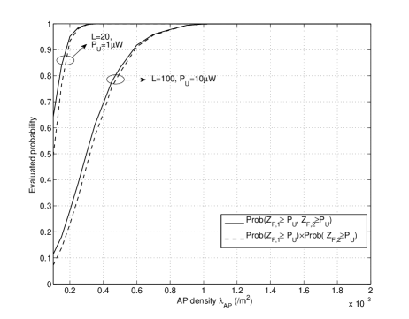
Figure 3: Validation of the independent assumption for $Z_{F}$’s.

First, we validate the feasibility of Assumption 1. Since the correlations between $Z_{F}$’s are similar over time frames and space $\mathbb{R}^{2}$, we focus on validating that $Z_{F}$’s can be viewed independent over space $\mathbb{R}^{2}$. Specifically, we randomly select two wireless nodes and index them with $i=1$ and $i=2$, respectively. The two wireless nodes independently and uniformly change their locations over frames in the interim square with length $L$m. We consider two scenarios, where in the first scenario, we set $L=20$m and $P_{U}=1\mu$W, and in the second scenario, we set $L=100$m and $P_{U}=10\mu$W. Clearly, both wireless nodes are of smaller mobility in the former scenario and larger mobility in the latter one. Moreover, since $L<\infty$, the two wireless nodes are of limited mobility over frames in both scenarios. In Fig. 3, we evaluate and compare the marginal probability product $\mathbb{P}(Z_{F,1}\geq P_{U})\times\mathbb{P}(Z_{F,2}\geq P_{U})$ with the joint probability $\mathbb{P}(Z_{F,1}\geq P_{U},Z_{F,2}\geq P_{U})$ over the AP density $\lambda_{AP}$ in both scenarios. It is observed from Fig. 3 that in both scenarios, for any AP density, the gap between the marginal probability product and the joint probability is tightly approaching zero; and especially when AP density is reasonably large, such gap decreases to be zero. Hence, the harvested energy of these two wireless nodes in one frame is tightly approaching to be independent, and thus can be viewed as independent. Moreover, by comparing the two scenarios, it is observed that when the wireless nodes are of smaller mobility in the first scenario, the gap between marginal probability product and the joint probability is comparatively large when $\lambda_{AP}$ is quite small (e.g., $\lambda_{AP}=0.0001/\textrm{m}^{2}$). This is mainly because when $\lambda_{AP}$ is quite small, the dominate APs are more correlated for wireless nodes with smaller mobility, as compared to that with larger mobility. However, the resulted correlation is rapidly reduced as $\lambda_{AP}$ is reasonably increased. Therefore, Assumption 1 can be well applied in the considered WPCN.

Next, we validate the Poisson assumption for the point process formed by the active wireless nodes in the UL slot. According to [14], a point process on $\mathbb{R}^{2}$ is fully characterized by its void probability on an arbitrary compact subset of $\mathbb{R}^{2}$. We evaluate and compare the void probability of the actual point process in the UL slot with that of the assumed PPP $\Phi(\lambda_{a})$ in the interim square with side length $L$, by setting $L=1:1:20$, in Fig. 4. From [14], given $L$, the void probability of $\Phi(\lambda_{a})$ in the interim square is given by $\exp\left(-\lambda_{a}L^{2}\right)$. We set $\lambda_{AP}=0.0005/\textrm{m}^{2}$ and $P_{U}=10\mu$W. It is observed from Fig. 4 that the void probabilities of both the assumed PPP and the actual point process in the UL decrease over the increased interim area with side length $L$, as expected. Moreover, since Assumption 1 can be well applied, as its direct result to obtain the PPP $\Phi(\lambda_{a})$ in the UL, it is observed that for any $L$, the void probability of the assumed PPP $\Phi(\lambda_{a})$ is tightly close to that of the actual point process in the UL, which validates the PPP assumption for the point process in the UL. In addition, from (8) and (9), since the density $\lambda_{a}$ is determined by the distribution of $Z_{F}$, the successful validation of the assumed PPP $\Phi(\lambda_{a})$ also implies the correctness of the derived $Z_{F}$’s distribution in Proposition 2.1 under Assumption 1.

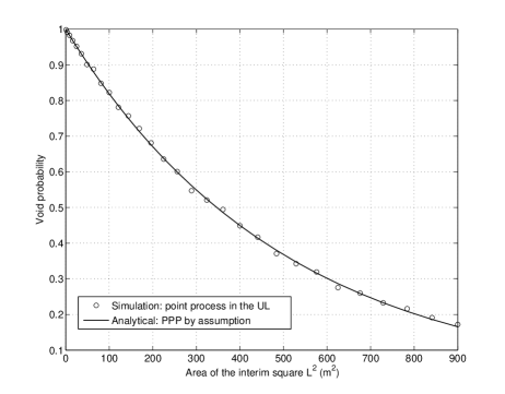
Figure 4: Validation of the PPP assumption for the point process in the UL.

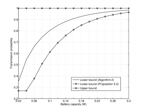
Figure 5: Transmission probability over battery capacity.

VI-B Study on Transmission Probability and Spatial Throughput

This subsections studies the transmission probability and the spatial throughput. Unless otherwise specified, in this subsection, we reasonably set $P_{D}=10$W, $\sigma^{2}=-60$dBm, $\epsilon=0.05$, $\eta=0.4$, $T=100$, and $\beta=5$. Moreover, we set $n=9$ for calculating $\textrm{erf}(x)$ in (17), where $v_{e}$ is obtained as $v_{e}=\textrm{erfinv}(10^{-9})$. Similarly, $g_{0}$ is obtained by numerically solving $g_{0}Q\left(\frac{g_{0}}{2\pi}\right)=(1-\epsilon)\exp\left(-\frac{g_{0}^{2}}{4\pi}\right)$ as given in Proposition III.2. We also observe that similar performance can be obtained by using other parameters.

VI-B1 Transmission Probability $\rho$

Since the transmission probabilities for the battery-free and infinite-capacity battery cases are obtained exactly, as given in (14) and (21), respectively, we focus on the transmission probability for the finite-capacity battery case. We set $\lambda_{w}=0.0012/m^{2}$, $\lambda_{AP}=0.0008/m^{2}$, $N=60$, and $P_{U}=0.02$W.

Fig. 5 compares the closed-form lower and upper bounds of $\rho$, given in Proposition V.2, and the tight lower bound, given by Algorithm 2, over the battery capacity $C$. By adopting Algorithm 2, we set the absolute error $\theta=0.001$, and initialize $\delta=0.0001$. First, it is observed from Fig. 5 that the tight lower bound by Algorithm 2 monotonically increases over battery capacity $C$ as expected; and as the actual transmission probability, it is bounded by the upper and lower bounds provided in Proposition V.2, respectively. Next, for the closed-form lower bound by Proposition V.2, it is observed when the capacity is small with $0.2\leq C\leq 0.4$, a constant lower bound is obtained as $\textrm{erf}\left(\frac{\Gamma(N+2/\alpha)\lambda_{AP}}{2\Gamma(N)}\sqrt{\frac{\pi^{3}P_{D}\eta}{P_{U}}}\right)\geq 1-e^{-Q(C-P_{U})}$; and when $C>0.4$, the lower bound is given by $1-e^{-Q(C-P_{U})}\geq\textrm{erf}\left(\frac{\Gamma(N+2/\alpha)\lambda_{AP}}{2\Gamma(N)}\sqrt{\frac{\pi^{3}P_{D}\eta}{P_{U}}}\right)$, which generally captures the variation of the transmission probability, by taking the tight lower bound by Algorithm 2 as a reference. Moreover, as $C$ increases, we observe both lower bounds by Algorithm 2 and Proposition V.2 approach to the upper bound $\rho=1$, and that by Algorithm 2 becomes tight to $\rho=1$ when $C$ is large. Furthermore, noticing that $\textrm{erf}\left(\frac{\Gamma(N+2/\alpha)\lambda_{AP}}{2\Gamma(N)}\sqrt{\frac{\pi^{3}P_{D}\eta}{P_{U}}}\right)$ is the transmission probability in the battery-free case, given in (14), we observe that it is always lower than the tight lower bound by Algorithm 2 in the battery-deployed case as expected.

VI-B2 Spatial Throughput

We study the spatial throughput in both battery-free and battery-deployed cases. In the battery-free case, by applying Theorem IV.1, we focus on showing the effects of the AP density $\lambda_{AP}$ and wireless node density $\lambda_{w}$ on the maximized spatial throughput. In the battery-deployed case, we focus on the challenging finite-capacity battery case with $\lambda_{AP}<\frac{2v_{e}\Gamma(N)}{\Gamma(N+2/\alpha)}\sqrt{\frac{P_{U}}{\pi^{3}P_{D}\eta}}$, and exploit Algorithm 2 to help find the maximized spatial throughput.

Fig. 6 shows the maximized spatial throughput over the AP density in the battery-free case, by applying Theorem IV.1. We consider two scenarios, with wireless node density $\lambda_{w}=0.0012/m^{2}$ and $\lambda_{w}=0.002/m^{2}$, respectively, where for each scenario, the low, medium and high AP regimes are given by $\big{[}0,\lambda_{w}/(K_{\epsilon}(T-1)\big{)}$, $\big{[}\lambda_{w}/(K_{\epsilon}(T-1)),\lambda_{w}/K_{\epsilon}\big{)}$, and $\big{[}\lambda_{w}/K_{\epsilon},\infty\big{)}$, respectively. First, for both scenarios, it is observed that by increasing $\lambda_{AP}$, the maximized spatial throughput slowly increases in the low AP density regime, and after $\lambda_{AP}=\lambda_{w}/(K_{\epsilon}(T-1))$, it rapidly increases in the medium AP density regime and achieves its maximum achievable spatial throughput $\lambda_{w}\log_{2}(1+\beta)$ at some point in this regime; and after this point, it remains as the constant $\lambda_{w}\log_{2}(1+\beta)$ over all the medium and high AP density regimes. Since in both scenarios, we observe that $\lambda_{w}\log_{2}(1+\beta)$ is achieved far before $\lambda_{AP}$ reaches to its high density regime, for ease of illustration, we only show the low AP density regime and part of the medium AP density regime in Fig.  6 for both scenarios. Next, it is observed that the maximum achievable spatial throughput $\lambda_{w}\log_{2}(1+\beta)$ is larger for the scenario with a larger $\lambda_{w}=0.002/m^{2}$, as compared to the scenario with $\lambda_{w}=0.0012/m^{2}$. Moreover, in the scenario with a larger $\lambda_{w}=0.002/m^{2}$, due to the increased interference level, to achieve $\lambda_{w}\log_{2}(1+\beta)$ under the successful information transmission probability constraint, more APs are needed to be deployed to reduce the distance between the wireless nodes and their associated APs, so as to improve the desired signal strength and thus the successful information transmission probability.

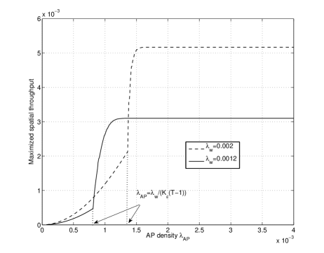
Figure 6: Maximized spatial throughput over $\lambda_{AP}$ in battery-free case.

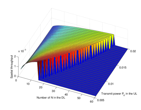
Figure 7: Spatial throughput over feasible region in finite-capacity battery case.

Fig. 7 shows the spatial throughput for the finite-capacity battery case over $N$ and $P_{U}$, where we set $T=100$, $P_{\max}=0.02$W, $C=0.04$W, $\lambda_{w}=0.0012/m^{2}$, and $\lambda_{AP}=0.0008/m^{2}$. By applying Algorithm 2 with $\theta=0.001$ and initialized $\delta=0.0001$, we use the method presented in Section V-B3 to compute $R^{LB}(N,P_{U})$ over all feasible $N$ and $P_{U}$, and take the obtained $R^{LB}(N,P_{U})$ as a tight approximation to $R(N,P_{U})$. We find the optimal solutions that maximize $R^{LB}(N,P_{U})$ are $N^{*}=14$ and $P_{U}^{*}=P_{min}=0.0055$W in Fig. 7. Thus, similar to the battery-free case in Theorem IV.1, the wireless nodes prefer to choose $P_{min}$, which assures a large transmission probability $\rho$. Moreover, with small $N^{*}=14$ in the DL phase, the UL phase is assigned with $T-N^{*}=86$ slots, which helps effectively reduce the UL interference by the independent scheduling. In addition, since a smaller $P_{U}$ yields an increased $\rho$, and thus requires a smaller $N$ to satisfy the transmission probability constraint in Problem (P2), it is observed from Fig. 7 that the feasible region of $N$ becomes smaller as $P_{U}$ decreases.

VII Conclusion

In this paper, we studied the optimal tradeoff between the energy transfer and information transfer in a large-scale WPCN, for both battery-free and battery-deployed wireless nodes. We proposed a new time-partition-based harvest-then-transmit protocol and modeled the network based on homogeneous PPPs. By using tools from stochastic geometry, we characterized the distribution of the harvested energy in the DL and the successful information transmission probability in the UL. We studied the resulting transmission probability and successfully solved the spatial throughput maximization problem for both battery-free and battery-deployed cases. Moreover, by comparing the network performance in the battery-free, infinite-capacity battery, and finite-capacity battery cases, we investigated the effects of battery storage on the system spatial throughput.

Appendix A Proof of Proposition III.2

We first present three lemmas.

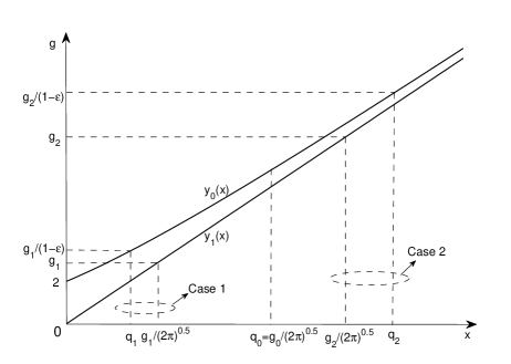
Figure 8: Illustration of $y_{0}(x)=\frac{g}{1-\epsilon}$ and $y_{1}(x)=g$.

Lemma A.1

For any $x\geq\frac{g}{\sqrt{2\pi}}$, $g\geq 0$, $g\exp\left(\frac{x^{2}}{2}\right)Q(x)\geq 1-\epsilon$ is equivalent to $x\leq q$ with $\frac{g}{\sqrt{2\pi}}\leq q$, where $q$ is the unique solution to $g\exp\left(\frac{q^{2}}{2}\right)Q(q)=1-\epsilon$.

Proof:

Let $y_{0}(x)=\frac{\exp\left(\frac{-x^{2}}{2}\right)}{Q(x)}$. It is easy to verify that $y_{0}(x)$ monotonically increases over $x\geq 0$, as shown in Fig. 8. As a result, $g\exp\left(\frac{x^{2}}{2}\right)Q(x)\geq 1-\epsilon$ is equivalent to $x\leq q$. Moreover, since $x\geq\frac{g}{\sqrt{2\pi}}$, we need $\frac{g}{\sqrt{2\pi}}\leq q$; otherwise, no valid $x\in[\frac{g}{\sqrt{2\pi}},q]$ exists to meet $g\exp\left(\frac{x^{2}}{2}\right)Q(x)\geq 1-\epsilon$. Lemma A.1 thus follows. ∎

Lemma A.2

$\frac{g}{\sqrt{2\pi}}\leq q$ is equivalent to $g\geq g_{0}$.

Proof:

Let $y_{1}(x)\!=\!\sqrt{2\pi}x$. While $q$ is the unique solution to $y_{0}(x)\!=\!\frac{g}{1-\epsilon}$, we have $\frac{g}{\sqrt{2\pi}}$ is the unique solution to $y_{1}(x)\!=\!g$. Notice that $q$ is a function of $g$, and as shown in Fig. 8, when $g$ increases, both $q$ and $\frac{g}{\sqrt{2\pi}}$ increase. First, since $g_{0}$ is the unique solution to $\frac{g_{0}}{1-\epsilon}\!=\!\frac{\exp\left(-g_{0}^{2}/4\pi\right)}{Q\left(g_{0}/2\pi\right)}$, it is easy to obtain that when $g\!=\!g_{0}$, $q_{0}\!=\!\frac{g_{0}}{\sqrt{2\pi}}$ is the unique solution to $\frac{g_{0}}{1-\epsilon}\!=\!\frac{\exp\left(-q_{0}^{2}/2\right)}{Q(q_{0})}$. In other words, when $g\!=\!g_{0}$, we obtain $q\!=\!\frac{g}{\sqrt{2\pi}}$. Next, by expanding $Q(x)$, we have $Q(x)\!=\!\frac{1}{\sqrt{2\pi}}\exp\left(-\frac{x^{2}}{2}\right)\left[\frac{1}{x}-\frac{1}{x^{2}}+o(x^{-4})\right]$. We thus can easily obtain $y_{0}(x)\geq y_{1}(x)$, and $\lim_{x\rightarrow\infty}y_{0}(x)\!=\!y_{1}(x)$, i.e., $y_{0}(x)$ and $y_{1}(x)$ are getting closer as $x$ increases. As a result, as illustrated in Fig. 8, it is easy to verify the followings: 1) when $g<g_{0}$, due to the big gap between $y_{0}(x)$ and $y_{1}(x)$, we have $q<\frac{g}{\sqrt{2\pi}}$, as illustrated by Case 1 with $g=g_{1}$ and $q=q_{1}$; and 2) due to the increasingly small gap between $y_{0}(x)$ and $y_{1}(x)$ as $g$ increases, when $g>g_{0}$, we have $q>\frac{g}{\sqrt{2\pi}}$, as illustrated by Case 2 with $g=g_{2}$ and $q=q_{2}$. Lemma A.2 thus follows. ∎

Lemma A.3

When $g\geq g_{0}$, we have $\frac{\exp\left(-\frac{x^{2}}{2}\right)}{Q(x)}=\sqrt{2\pi}x$, as $\epsilon\rightarrow 0$.

Proof:

It has been shown from the proof of Lemma A.2 that $\frac{\exp\left(-\frac{x^{2}}{2}\right)}{Q(x)}\!>\!\sqrt{2\pi}x$. On the other hand, when $g\!\geq\!g_{0}$, since $q\!\geq\!\frac{g}{\sqrt{2\pi}}$, we have $\frac{\exp\left(-\frac{x^{2}}{2}\right)}{Q(x)}\Big{|}_{x=\frac{g}{\sqrt{2\pi}}}\!\leq\!\frac{\exp\left(-\frac{x^{2}}{2}\right)}{Q(x)}\Big{|}_{x=q}\!=\!\frac{g}{1-\epsilon}$, or equivalently, $\frac{\exp\left(-\frac{x^{2}}{2}\right)}{Q(x)}\leq\frac{\sqrt{2\pi}x}{1-\epsilon}$, by substituting $g\!=\!\sqrt{2\pi}x$. As a result, $\frac{\exp\left(-\frac{x^{2}}{2}\right)}{Q(x)}\!=\!\sqrt{2\pi}x$, as $\epsilon\rightarrow 0$. Lemma A.3 thus follows. ∎

Therefore, since $\Upsilon\geq\frac{G}{\sqrt{2\pi}}$ in (12), from Lemma A.1 and Lemma A.2, (12) is equivalent to $\Upsilon\leq q$ with $G\geq g_{0}$. From Lemma A.3, we can obtain $q=\frac{G}{(1-\epsilon)\sqrt{2\pi}}$ with $\epsilon\rightarrow 0$. By substituting the expression of $\Upsilon$ and $G$, we find $P_{suc}\geq 1-\epsilon$ is equivalent to the transmission probability constraint with $P_{U}\geq\frac{g_{0}^{2}\beta\sigma^{2}}{\pi^{3}\lambda_{AP}^{2}}$. Proposition III.2 thus follows.

Appendix B Proof of Theorem IV.1

Note that in the first constraint of (P3), for the left-hand side, we have $\lambda_{w}\textrm{erf}\left(\frac{\Gamma(N+2/\alpha)\lambda_{AP}}{2\Gamma(N)}\sqrt{\frac{\pi^{3}P_{D}\eta}{P_{U}}}\right))\leq\lambda_{w}$, and for the right-hand side, we have $K_{\epsilon}\lambda_{AP}\leq K_{\epsilon}\lambda_{AP}(T-N)\leq K_{\epsilon}\lambda_{AP}(T-1)$. Thus, by comparing the upper bound of $\lambda_{w}\textrm{erf}\left(\frac{\Gamma(N+2/\alpha)\lambda_{AP}}{2\Gamma(N)}\sqrt{\frac{\pi^{3}P_{D}\eta}{P_{U}}}\right)$ with the upper and lower bounds of $K_{\epsilon}\lambda_{AP}(T-N)$, respectively, we obtain the following three regimes of the AP density $\lambda_{AP}$:

1. If $\lambda_{w}\leq K_{\epsilon}\lambda_{AP}$, i.e., in the high AP density regime, it is clear the first constraint in Problem (P3) can always hold. Thus, any $N\in\{1,...,T-1\}$ and $P_{U}\in[P_{\min},P_{\max}]$ are feasible to Problem (P3). Note that $R(N,P_{U})$ achieves its maximum value when $N=T-1$ and $P_{U}=P_{\min}$. As a result, if $N=T-1$ and $P_{U}=P_{\min}$ satisfy (18) for assuring $\rho=1$, we find any pair of $N^{*}$ and $P_{U}^{*}$ that satisfy (18) are optimal to Problem (P3), and $R(N^{*},P_{U}^{*})=\lambda_{w}\log(1+\beta)$; otherwise, we have $\rho<1$ and thus $R(N^{*},P_{U}^{*})<\lambda_{w}\log(1+\beta)$, with $N^{*}=T-1$ and $P_{U}^{*}=P_{\min}$.

2. If $K_{\epsilon}\lambda_{AP}<\lambda_{w}\leq K_{\epsilon}\lambda_{AP}(T-1)$, i.e., in the medium AP density regime, a unique $N_{0}$ clearly exists, since otherwise, the condition $K_{\epsilon}\lambda_{AP}<\lambda_{w}\leq K_{\epsilon}\lambda_{AP}(T-1)$ cannot hold. It is thus easy to verify that the first constraint in Problem (P3) holds if and only if $N\leq N_{0}$. As a result, the feasible region for Problem (P3) is given by any $N\in\{1,...,N_{0}\}$ and $P_{U}\in[P_{\min},P_{\max}]$. At last, by using the similar method as in the case of high AP density regime, we can easily find $N^{*}$, $P_{U}^{*}$ and $R(N^{*},P_{U}^{*})$ as stated in Theorem IV.1.

3. If $\lambda_{w}>K_{\epsilon}\lambda_{AP}(T-1)$, i.e., in the low AP density regime, if $\lambda_{w}\textrm{erf}\left(\frac{\Gamma(N+2/\alpha)\lambda_{AP}}{2\Gamma(N)}\sqrt{\frac{\pi^{3}P_{D}\eta}{P_{max}}}\right)>K_{\epsilon}\lambda_{AP}(T-N)$ at $N=1$, which gives the largest value of the right-hand side in the first constraint of (P3), the first constraint of Problem (P3) cannot hold, and thus there is no feasible solution; otherwise, there exists optimal $N^{*}$ and $P_{U}^{*}$, which yield $\rho<1$. As shown in Algorithm 1, since for any given $N$, $\lambda_{w}\textrm{erf}\left(\frac{\Gamma(N+2/\alpha)\lambda_{AP}}{2\Gamma(N)}\sqrt{\frac{\pi^{3}P_{D}\eta}{P_{U}}}\right)$ achieves its minimum value when $P_{U}=P_{\max}$, we use $\lambda_{w}\textrm{erf}\left(\frac{\pi^{2}\lambda_{AP}N}{4}\sqrt{\frac{P_{D}\eta}{P_{\max}}}\right)\leq K_{\epsilon}\lambda_{AP}(T-N)$ to check whether an $N$ is feasible, by searching over $N\in\{1,...,T-1\}$. After finding a feasible $N$, we then calculate the corresponding $P_{U}=\max(P_{s},P_{\min})$ that maximizes $R(N,P_{U})$. Finally, by comparing all the feasible $N$’s and their corresponding $P_{U}$’s, we can find optimal $N^{*}$ and $P_{U}^{*}$ that maximizes $R(N,P_{U})$. Clearly, by searching over $N\in\{1,...,T-1\}$, Algorithm 1 is of complexity or of $\mathcal{O}(T)$.

Based on the above three cases, Theorem IV.1 thus follows.

Appendix C Proof of Proposition V.1

We note a different proof based on random walk theory for Proposition V.1 was provided in [21]. Compared to [21], by exploiting the distribution of $Z_{F}$, the proof presented in the following is much simpler. From (2), we have

$$S_{F}=\sum_{i=1}^{F}Z_{i}-P_{U}\sum_{i=1}^{F}I(S_{i-1}\geq P_{U})\geq\sum_{i=1}^{F}Z_{i}-FP_{U}.$$ (30)

Under Assumption 1 with i.i.d. $Z_{F}$’s, it is easy to verify that the point processes at the end of the DL phase of each frame are i.i.d. PPPs, each with density $\lambda_{AP}$. Thus, $\sum_{i=1}^{F}Z_{i}$ gives the harvested energy over all $F$ i.i.d PPPs, which is equivalent to the harvested energy in a PPP of density $F\lambda_{AP}$. Hence, we can easily obtain that for any given $z\geq 0$, $\mathbb{P}\left(\sum_{i=1}^{F}Z_{i}\geq z\right)=\textrm{erf}\left(\frac{\Gamma(N+2/\alpha)F\lambda_{AP}}{2\Gamma(N)}\sqrt{\frac{\pi^{3}P_{D}\eta}{P_{U}}}\right)$, which is equal to $1$ when $F$ is sufficiently large. As a result, from (8) and (30), we obtain

$$\rho \geq\lim_{n\to\infty}\frac{1}{n}\sum_{F=1}^{n}\mathbb{P}\left(\sum_{i=1}^{F}Z_{i}\geq(F+1)P_{U}\right)$$

$$=\lim_{n\to\infty}\frac{1}{n}\sum_{F=1}^{n}\textrm{erf}\left(\frac{\Gamma(N+2/\alpha)F\lambda_{AP}}{2\Gamma(N)}\sqrt{\frac{\pi^{3}P_{D}\eta}{P_{U}}}\right)$$

$$=1.$$ (31)

Since $\rho\leq 1$, we have $\rho=1$. Proposition V.1 thus follows.

Appendix D Proof of Proposition V.2

Since both $\textrm{erf}\left(\frac{\pi^{2}\lambda_{AP}N}{4}\sqrt{\frac{P_{D}\eta}{P_{U}}}\right)$ and $1-e^{-Q(C-P_{U})}$ are lower bounds of $\rho\leq 1$, it is easy to find that $\mathcal{L}\leq\rho\leq 1$ holds. This proof mainly derives the expression of $Q$ by solving $\ln\mathbb{E}\left[e^{-Q(Z_{F}-P_{U})}\right]=0$, or equivalently, $\mathbb{E}\left(e^{-QZ_{F}}\right)=e^{-QP_{U}}$. From the Laplace transform of $Z_{F}$ given in Proposition II.1, it is easy to find that $\mathbb{E}\left(e^{-QZ_{F}}\right)=\exp\left(-\pi\lambda_{AP}\frac{\Gamma(N+2/\alpha)}{\Gamma(N)}\Gamma(1-2/\alpha)(P_{D}\eta Q)^{2/\alpha}\right)$, and thus $Q$ by letting $\mathbb{E}\left(e^{-QZ_{F}}\right)=e^{-QP_{U}}$. Proposition V.2 thus follows.

References

- [1] R. J. M. Vullers, R. V. Schaijk, I. Doms, C. V. Hoof, and R. Mertens, “Micropower energy harvesting,” Elsevier Solid-State Circuits, vol. 53, no. 7, pp. 684-693, Jul. 2009.
- [2] H. J. Visser and R. J. Vullers, “RF energy harvesting and transport for wireless sensor network applications: Principles and requirements,” Proc. IEEE, vol. 101, no. 6, pp. 1410–1423, Apr. 2013.
- [3] A. M. Zungeru, L. M. Ang, S. Prabaharan, and K. P. Seng, “Radio frequency energy harvesting and management for wireless sensor networks,” Green Mobile Devices Netw.: Energy Opt. Scav. Tech., CRC Press, pp. 341-368, 2012.
- [4] S. He, J. Chen, F. Jiang, D. Yau, G. Xing, and Y. Sun, “Energy provisioning in wireless rechargeable sensor networks,” IEEE Trans. Mob. Comput., vol. 12, no. 10, pp. 1931-1942, Oct. 2013.
- [5] H. Ju and R. Zhang, “Throughput maximization in wireless powered communication networks,” IEEE Trans. Wireless Commun., vol. 13, no. 1, pp. 418-428, Jan. 2014.
- [6] O. Ozel, K. Tutuncuoglu, J. Yang, S. Ulukus, and A. Yener, “Transmission with energy harvesting nodes in fading wireless channels: Optimal policies,” IEEE J. Sel. Areas Commun., vol. 29, no. 8, pp. 1732-1743, Sep. 2011.
- [7] C. K. Ho and R. Zhang, “Optimal energy allocation for wireless communications with energy harvesting constraints,” IEEE Trans. Sig. Process., vol. 60, no. 9, pp. 4808-4818, Sep. 2012.
- [8] J. Xu and R. Zhang, “Throughput optimal policies for energy harvesting wireless transmitters with non-ideal circuit power,” IEEE J. Sel. Areas Commun., vol. 32, no. 2, pp. 322-332, Feb. 2014.
- [9] R. Zhang and C. K. Ho, “MIMO broadcasting for simultaneous wireless information and power transfer,” IEEE Trans. Wireless Commun., vol. 12, no. 5, pp. 1989-2001, May 2013.
- [10] L. Liu, R. Zhang, and K. C. Chua, “Wireless information transfer with opportunistic energy harvesting,” IEEE Trans. Wireless Commun., vol. 12, no. 1, pp. 288-300, Jan. 2013.
- [11] Y. C. Jin, Y. G. Wen, and Q. H. Chen, “Energy efficiency and server virtualization in data centers: An empirical investigation,” IEEE INFOCOM Workshop on Communications and Control for Sustainable Energy Systems: Green Networking and Smart Grids, Mar. 2012.
- [12] Y. C. Jin, Y. G. Wen, Z. Q. Zhu, and Q. H. Chen, “ An empirical investigation of the impact of server virtualization on energy efficiency for green data center,” The Computer Journal, Oxford Journals, vol. 51, no. 8, pp. 968-975, Aug. 2013.
- [13] W. W. Zhang, Y. G. Wen, K. Guan, D. Kilper, H. Y. Luo, and D. P. Wu, “Energy-efficient mobile computing under stochastic wireless channel,” IEEE Trans. Wireless Commun., vol. 12, no. 9, pp. 4569-4581, Sep. 2013.
- [14] D. Stoyan, W. S. Kendall, and J. Mecke, Stochastic geometry and its applications, 2nd edition. John Wiley and Sons, 1995.
- [15] M. Haenggi and R. K. Ganti, Interference in large wireless networks. NOW: Foundations and Trends in Networking, 2008.
- [16] K. Huang and V. K. N. Lau, “Enabling wireless power transfer in cellular networks: architecture, modeling and deployment,” IEEE Trans. Wireless Commun., vol. 13, no. 2, pp. 902-912, Feb. 2014.
- [17] S. Lee, R. Zhang, and K. Huang, “Opportunistic wireless energy harvesting in cognitive radio networks,” IEEE Trans. Wireless Commun., vol. 12, no. 9, pp. 4788-4799, Sep. 2013.
- [18] Available [online] at http://witricity.com/applications/military.
- [19] L. Xie, Y. Shi, Y. T. Hou, and H. D. Sherali, “Making sensor networks immortal: an energy-renewable approach with wireless power transfer,” IEEE/ACM Trans. Netw., vol. 20, no. 6, pp. 1748-1761, Dec. 2012.
- [20] Y. L. Che, R. Zhang, Y. Gong and L. Duan, “On spatial capacity of wireless ad hoc networks with threshold based scheduling,” IEEE Trans. Wireless Commun., vol. 13, no. 12, pp. 6915-6927, Oct. 2014.
- [21] K. Huang, “Spatial throughput of mobile ad hoc networks with energy harvesting,” IEEE Trans. Inf. Theory, vol. 59, no. 11, pp. 7597-7612, Nov. 2013.
- [22] H. S. Dhillon, Y. Li, P. Nuggehalli, Z. Pi, and J. G. Andrews, “Fundamentals of heterogeneous cellular networks with energy harvesting”, IEEE Trans. Wireless Commun., vol. 13, no. 5, May 2014.
- [23] A. P. Sample, D. J. Yeager, P. S. Powledge, and J. R. Smith, “Design of a passively-powered, programmable platform for UHF RFID systems,” in Proc. IEEE Int. Conf. RFID, Mar. 2007.
- [24] A. Sample and J. R. Smith, “Experimental results with two wireless power transfer systems,” in IEEE Radio Wireless Symp., Jan. 2009.
- [25] Product datasheet P2110-915 MHz RF powerharvester receiver. Available [online] at http://www.powercastco.com/PDF/P2110-datasheet.pdf.
- [26] W. W. Zhang, Y. G. Wen, and D. P. Wu, “Energy-efficient scheduling policy for collaborative execution in mobile cloud computing,” in Proc. IEEE Int. Conf. Computer Commun. (INFOCOM), Apr. 2013.
- [27] J. G. Andrews, F. Baccelli, and R. K. Ganti, “A tractable approach to coverage and rate in cellular networks,” IEEE Trans. Commun., vol. 59, no. 11, pp. 3122-3134, Nov. 2011.
- [28] F. Baccelli and B. Blaszczyszyn, Stochastic Geometry and Wireless Networks, Volume I: Theory. NOW: Foundations and Trends in Networking, 2009.
- [29] Z. Gong and M. Haenggi, “Interference and outage in mobile random networks: expectation, distribution, and correlation,” IEEE Trans. Mob. Comput., vol. 13, pp. 337-349, Feb. 2014.
- [30] S. P. Weber and M. Kam, “Computational complexity of outage probability simulations in mobile ad-hoc networks,” in Proc., Conf. on Information Sciences and Systems, Mar. 2005.