Area-preserving maps models of gyroaveraged
${\bf E}\times{\bf B}$ chaotic transport

Abstract

Discrete maps have been extensively used to model 2-dimensional chaotic transport in plasmas and fluids. Here we focus on area-preserving maps describing finite Larmor radius (FLR) effects on $E\times B$ chaotic transport in magnetized plasmas with zonal flows perturbed by electrostatic drift waves. FLR effects are included by gyro-averaging the Hamiltonians of the maps which, depending on the zonal flow profile, can have monotonic or non-monotonic frequencies. In the limit of zero Larmor radius, the monotonic frequency map reduces to the standard Chirikov-Taylor map, and, in the case of non-monotonic frequency, the map reduces to the standard nontwist map. We show that in both cases FLR leads to chaos suppression, changes in the stability of fixed points, and robustness of transport barriers. FLR effects are also responsible for changes in the phase space topology and zonal flow bifurcations. Dynamical systems methods based on recurrence time statistics are used to quantify the dependence on the Larmor radius of the threshold for the destruction of transport barriers.

I Introduction

Important research efforts in controlled nuclear fusion are focused on the magnetic confinement of hot plasmas. In order to improve the confinement conditions, a better understanding of the particle transport is needed, especially in the case of particle drift motion. A standard approach to this problem is based on the $\vec{E}\times\vec{B}$ approximation of charged particle’s guiding center’s motion, e.g. Refs. kleva-drake-1984 ; Pettini ; ibere_horton_2008 ; del-castillo-2000 . However, in the case of fast particles, e.g. alpha particles in burning plasmas, or in the presence of inhomogeneous fields on the scale of the Larmor radius, it is necessary to consider finite Larmor radius (FLR) effects to correctly estimate the transport of particles Manfredi96 ; del-castillo-martinell2013 .

Previous studies on the role of the Larmor radius on transport include Refs. Annibaldi02 ; Manfredi96 ; Manfredi97 where particle transport in numerical simulations of electrostatic turbulence was analyzed and FLR effects were shown to inhibit transport. The problem of non-diffusive chaotic transport and fractional diffusion in the presence of FLR effects was addressed in Ref. gustafson . In Refs. del-castillo-martinell2012 ; del-castillo-martinell2013 dynamical systems methods were used to investigate FLR effects on chaos suppression and bifurcations in the phase space topology.

In this paper we study FLR effects in the context of simplified area-preserving map models of $\vec{E}\times\vec{B}$ motion. The maps are constructed following the standard Hamiltonian framework for electrostatic drift motion horton-1985 , and FLR corrections are included by gyro-averaging the electrostatic potential Lee87 . The potential has an equilibrium depending on the radial coordinate and a time-dependent perturbation consisting of a linear superposition of drift waves. Depending on the radial dependence of the equilibrium the maps’ frequencies can have monotonic or non-monotonic profiles. Our main focus is the study of FLR effects on chaos suppression, stability of fixed points, nontwist phase space topologies, and transport barriers. Although $\nabla\vec{B}\times\vec{B}$ drift might play a role in the presence of FLR, here we will restrict attention to $\vec{E}\times\vec{B}$ drifts.

In dynamical systems theory, the term “nontwist” is used to designate Hamiltonian systems that violate the twist or non-degeneracy condition. A paradigmatic example is a perturbed system in which the frequency of the unperturbed part of the Hamiltonian is a non-monotonic function of the action. Nontwist Hamiltonian systems are found in many physical systems including $\mathbf{E}\times\mathbf{B}$ transport in magnetized plasmas del-castillo-2000 ; ibere_horton_2008 , magnetic fields with reverse shear in toroidal plasma devices Oda ; Balescu98 ; del-castillo-1992 ; Firpo2009 , and transport by traveling waves in shear flows del-castillo-1993 ; Beron-Vera10 ; Budyansky09 among others. The presence of nontwist transport barriers is among the most important properties of nontwist Hamiltonian systems. By nontwist transport barriers we mean a robust region of invariant circles, also called Kolmogorov-Arnold-Moser (KAM) curves, that are very resilient to breakup, i.e., they can survive even when the phase space is almost completely chaotic. This property, originally discovered in Refs. del-castillo-1993 ; del-castillo-negrete-etal-1996 , has also been referred to as strong KAM stability Rypina in the context of one-and-a-half degrees-of-freedom Hamiltonian systems, and has been the subject of several studies (see, for example, Portela07 ; Szezech09 ; Caldas ; de-la-Llave-2000 and references therein). Throughout this paper use the term “KAM curve” as a synonymous of “invariant circle” or “transport barrier”.

In this paper the maps correspond to Hamiltonians whose unperturbed frequencies can be monotonic or non-monotonic functions of the action variable. The latter case is characterized by the presence of nontwist transport barriers that can be destroyed or restored by changing the value of the Larmor radius. This property is directly related to the FLR suppression of chaotic transport studied in Refs. del-castillo-martinell2012 ; del-castillo-martinell2013 . Here we show that chaos suppression occurs when the Larmor radius is close to specific values for which invariant circles become very resilient to breakup. In the case of nontwist maps, the invariant circles forming the nontwist transport barrier are the easiest to restore and the hardest to break. One of the main goals of the present work is the numerical computation of the critical parameters for the breakup of nontwist barriers. To compute the breakup diagrams we follow the technique in Ref. Altmann which is based on the application of Slater’s theorem Slater to the recurrence properties of orbits. As shown in Refs. Altmann ; Zou , the recurrence properties of an orbit provide an efficient and accurate method to differentiate chaotic and non-chaotic motion. A recent example of the application of this technique to the standard nontwist map was presented in Ref. Abud .

The rest of the paper is organized as follows. The next section introduces a general area preserving map of gyro-averaged $\vec{E}\times\vec{B}$ transport. This model is the starting point for the specific cases studied in the subsequent sections. The first case, for which the frequency has a monotonic profile, is presented in Sec. III, where FLR effects on the transition to global chaos are analyzed. Section IV describes a case with a non-monotonic profile and discusses FLR effects on the stability of fixed points, phase space topology, and breakup diagrams. A second nontwist map is presented in Sec. V where FLR effects on zonal flow bifurcations are analyzed. Section VI presents the conclusions and a brief summary of the main results.

II Transport Model

The $\vec{E}\times\vec{B}$ drift velocity of the guiding center is given by Nicholson

$$\vec{v}_{GC}=\frac{\vec{E}\times\vec{B}}{B^{2}}\,.$$ (1)

Using $x$ as radial coordinate, and $y$ as poloidal coordinate, the equations of the $\vec{E}\times\vec{B}$ drift motion, $(\dot{x}(t),\dot{y}(t))=\vec{v}_{GC}$, can be written as the Hamiltonian system

$$\frac{dx}{dt}=-\frac{\partial H(x,y,t)}{\partial y}\,,\qquad\frac{dy}{dt}=\frac{\partial H(x,y,t)}{\partial x},$$ (2)

where

$$H(x,y,t)=\frac{\phi(x,y,t)}{B_{0}}\,,$$ (3)

$\phi$ is the electrostatic potential, and $B_{0}$ denotes the magnitude of the toroidal magnetic field, $\vec{B}=B_{0}\hat{e}_{z}$. As discussed in Ref. del-castillo-martinell2012 , finite Larmor radius (FLR) effects can be incorporated substituting the electrostatic potential by its average over a circle around the guide center

$$\langle\phi\left(x,y,t\right)\rangle_{\varphi}=\frac{1}{2\pi}\int_{0}^{2\pi}\phi(x+\rho\cos\varphi,\,y+\rho\sin\varphi,\,t)\,d\varphi,$$ (4)

where $\rho$ is the Larmor radius. Equation (4) corresponds to the well-known gyro-averaging operation Lee87 . The gyro-averaged Hamiltonian can then be defined as

$$\langle H(x,y,t)\rangle_{\varphi}=\frac{\langle\phi\left(x,y,t\right)\rangle_{\varphi}}{B_{0}}$$ (5)

and the gyro-averaged equations of motion (2) can be written as

$$\frac{dy}{dt}=\frac{\partial\langle H\rangle_{\varphi}}{\partial x},\qquad\frac{dx}{dt}=-\frac{\partial\langle H\rangle_{\varphi}}{\partial y}\,.$$ (6)

Following Ref. horton-1998 , we assume an electrostatic potential of the form

$$\phi\left(x,y,t\right)=\phi_{0}(x)+A\sum_{m=-\infty}^{+\infty}\cos(ky-m\omega_{0}t),$$ (7)

where $\phi_{0}(x)$ is the equilibrium potential, $A$, the amplitude of the drift waves, $k$ is the wave number, and $\omega_{0}$ is the fundamental frequency. Applying the gyro-average operation in Eq. (4) to Eq. (7), and substituting the result in Eq. (3), we obtain the Hamiltonian

$$\langle H(x,y,t)\rangle_{\varphi}=\langle H_{0}(x)\rangle_{\varphi}+\frac{A}{B_{0}}J_{0}\left(k\rho\right)\sum_{m=-\infty}^{+\infty}\cos\left(ky-m\omega_{0}t\right),$$ (8)

where $J_{0}$ is the zero-order Bessel function, and the integrable Hamiltonian $\langle H_{0}(x)\rangle_{\varphi}$ is defined as

$$\langle H_{0}(x)\rangle_{\varphi}=\frac{\langle\phi_{0}\left(x\right)\rangle_{\varphi}}{B_{0}}$$ (9)

Using the Fourier series representation of the Dirac delta function, Eq. (8) can be rewritten as

$$\langle H(x,y,t)\rangle_{\varphi}=\langle H_{0}(x)\rangle_{\varphi}+\frac{2\pi A}{B_{0}}J_{0}\left(k\rho\right)\cos(ky)\sum_{m=-\infty}^{+\infty}\delta(\omega_{0}t-2\pi m).$$ (10)

Let $x_{n}=x(t^{-}_{n})$ and $y_{n}=y(t^{-}_{n})$, with $t^{-}_{n}=\frac{2\pi n}{\omega_{0}}-\varepsilon$, $n\in\mathbb{N}$, and $\varepsilon\rightarrow 0^{+}$. Integrating Eq. (6) in the interval $(t^{-}_{n},t^{-}_{n+1})$ leads to the gyro-averaged drift wave map

$$x_{n+1} =x_{n}+\frac{2\pi kA}{\omega_{0}B_{o}}J_{0}\left(\hat{\rho}\right)\sin(ky_{n})$$ (11)

$$y_{n+1} =y_{n}+\frac{2\pi}{\omega_{0}}\Omega\left(x_{n+1}\right)$$ (12)

where $\hat{\rho}=k\rho$, and $\Omega\left(x\right)$ corresponds to the frequency associated to the integrable Hamiltonian in Eq. (9)

$$\Omega\left(x\right)=\frac{d\langle H_{0}(x)\rangle_{\varphi}}{dx}\,.$$ (13)

For $\rho=0$, $\Omega\left(x\right)=-E_{r}(x)/B_{0}$, where $E_{r}(x)$ is the radial component of the electric field. Depending on the equilibrium potential $\phi_{0}(x)$, which determines $E_{r}(x)$ and $\Omega\left(x\right)$, different area-preserving maps can be constructed from Eqs. (11) and (12). In the next sections, we discuss three different cases.

III Gyroaveraged standard map

As a first simple example we assume a monotonic linear frequency profile to construct the gyro-averaged standard map (GSM). This map is a modified version of the standard map, also known as the Chirikov-Taylor map chirikov79 ; taylor . To define the frequency in Eq. (12), we use the equilibrium potential

$$\phi_{0}(x)=\alpha\frac{\left(kx\right)^{2}}{2},$$ (14)

where $k$ is the wave number in Eq. (7), and $\alpha$ is a free parameter. Applying the gyro-average operation to Eq. (14) yields

$$\langle H_{0}(x)\rangle_{\varphi}=\frac{\alpha}{B_{0}}\left[\frac{\left(kx\right)^{2}}{2}+\frac{\hat{\rho}^{2}}{4}\right].$$ (15)

Substituting Eq. (15) in Eq. (13), we get the frequency

$$\Omega\left(x\right)=\frac{\alpha k^{2}}{B_{0}}x,$$ (16)

which does not depend on the Larmor radius, and has a monotonic profile. Introducing the non-dimensional variables

$$I=k\gamma x,\qquad\theta=ky\,,$$ (17)

and the constant

$$\gamma=\frac{2\pi\alpha k^{2}}{\omega_{0}B_{0}}\,,$$ (18)

we get, from Eq. (11) and Eq. (12), the gyro-averaged standard map (GSM)

$$I_{n+1}= I_{n}+K_{ef}\left(\hat{\rho}\right)\sin\theta_{n}$$ (19)

$$\theta_{n+1}= \theta_{n}+I_{n+1},\quad mod\quad 2\pi$$ (20)

where

$$K_{ef}=KJ_{0}\left(\hat{\rho}\right)$$ (21)

is the effective perturbation parameter and $K=\gamma^{2}A/\alpha$ is the perturbation parameter. For $\hat{\rho}=0$, $K_{ef}=K$, and the GSM reduces to the standard map.

The phase space of the GSM, as in the case of any area-preserving map, consists of periodic, quasiperiodic, and chaotic orbits. Quasiperiodic orbits cover densely invariant curves. The invariant curves around the elliptic fixed points form island chains, and the invariant curves that wind around the entire domain of the angle variable form invariant circles Meiss92 . The presence of KAM curves is of special interest because they preclude transport in the direction of the radial coordinate $x$, keeping chaotic orbits confined to specific regions of phase space.

According to Greene’s residue method Greene79 , the transition to global chaos in the standard map occurs when the absolute value of the perturbation parameter is equal to, or greater than, the critical value $K_{c}\simeq 0.9716$. That is, for $K\geq K_{c}$, all KAM curves are broken, and chaotic orbits can spread over all phase space (except in regions occupied by isolated islands). Larmor radius effects on the transition to global chaos in the GSM can be analyzed by defining the critical line dividing the $K-\hat{\rho}$ parameter space in two regions: one for which the phase space contains at least one KAM curve and another for which transition to global chaos has occurred. In the standard map, there is no dependence on $\hat{\rho}$, which means that the critical line is just a horizontal line defined at $K=K_{c}$, as indicated in Fig. 1. However, for the GSM, the critical line is determined by the condition $\left|K_{ef}\right|=K_{c}$ which implies

$$K=\frac{K_{c}}{\left|\,J_{0}(\hat{\rho})\right|}$$ (22)

As shown in Fig. 1, even for high values of the perturbation parameter ($K\gg K_{c}$) there are an infinite number of regions of Larmor radius values for which KAM curves can be restored and chaos is suppressed. The gyro-averaging operation “breaks” the critical line at the zeros of the zero-order Bessel function. In particular, near the zeros, the critical perturbation goes to infinity and the transition to global chaos cannot occur. Writing $\hat{\rho}=\rho_{i}+\delta\hat{\rho}$, where $\rho_{i}$ is the $i$-th zero of $J_{0}$ and $\delta\hat{\rho}\ll 1$, and expanding in Taylor series, the divergence of the critical perturbation near the zeros of $J_{0}$ can be approximated as

$$K\approx\frac{K_{c}/|J_{1}(\rho_{i})}{|\hat{\rho}-\rho_{i}|}\,,$$ (23)

where $J_{1}$ denotes the Bessel function of first order. The first five positive zeros, indicated in Fig.  1, are approximately $\rho_{1}=2.40$, $\rho_{2}=5.52$, $\rho_{3}=8.65$, $\rho_{4}=11.79$, and $\rho_{5}=14.93$.

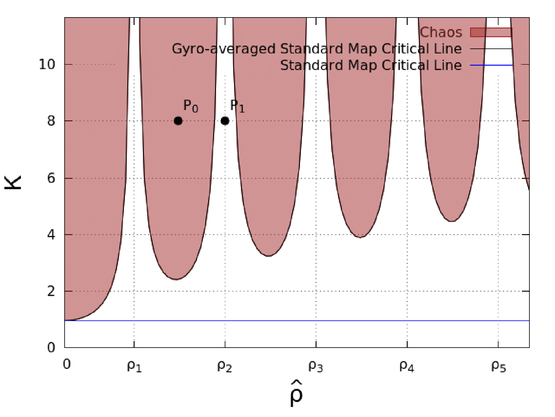
Figure 1: Critical lines for the standard map (blue horizontal line) and for the gyro-averaged standard map (black curves). Inside the shaded regions there is global chaos. (Color online)

The effect of chaos suppression is illustrated by Figs. 2 (a)-(b). Figure 2-(a) shows a GSM Poincaré section for $\hat{\rho}=3.9$ and $K=8.0$, which correspond to the point $P_{0}$ in Fig. 1. No KAM curves are observed in the Poincaré section as $P_{0}$ belongs to the region of global chaos. Keeping the same value of $K$ and changing the value of $\hat{\rho}$ to $\rho_{2}$ (point $P_{1}$ in Fig. 1) eliminates all the chaotic orbits (see figure 2(b)).

IV Gyroaveraged standard nontwist map

As a second example of the gyro-averaged drift wave map, we introduce the gyroaveraged standard nontwist map (GSNM), which corresponds to a non-monotonic radial electric field. In this case the equilibrium potential is

$$\phi_{0}(x)=\alpha\left[\left(\frac{x}{L}\right)-\frac{1}{3}\left(\frac{x}{L}\right)^{3}\right],$$ (24)

where $\alpha$ and $L$ are dimensional constants. The gyro-average of Eq. (24) gives

$$\langle H_{0}(x)\rangle_{\varphi}=\frac{\alpha}{B_{0}}\left[\left(\frac{x}{L}\right)\left(1-\frac{\rho^{2}}{2L^{2}}\right)-\frac{1}{3}\left(\frac{x}{L}\right)^{3}\right],$$ (25)

and from Eq. (13) we get the non-monotonic parabolic frequency profile,

$$\Omega\left(x\right)=\frac{\alpha}{B_{0}L}\left\{\left[1-\left(\frac{\rho}{\sqrt{2}L}\right)^{2}\right]-\left(\frac{x}{L}\right)^{2}\right\}\,,$$ (26)

which has a maximum at $x=0$. For $\rho=0$, the zeros of $\Omega\left(x\right)$ (and also of the $E_{r}$ profile) are located at $\pm L$, where $L$ is the characteristic length of the frequency profile. Substituting Eq. (26) into Eq. (12), we obtain

$$x_{n+1}= x_{n}+\frac{2\pi}{\omega_{0}B_{0}}AkJ_{0}\left(k\rho\right)\sin\left(ky_{n}\right)$$ (27)

$$y_{n+1}= y_{n}+\frac{2\pi}{\omega_{0}B_{0}}\frac{\alpha}{L}\left\{\left[1-\left(\frac{\rho}{\sqrt{2}L}\right)^{2}\right]-\left(\frac{x_{n+1}}{L}\right)^{2}\right\}.$$ (28)

Introducing the dimensionless variables:

$$I=-\frac{x}{L},\qquad\theta=\frac{ky}{2\pi},$$ (29)

we get the gyro-averaged standard nontwist map (GSNM):

$$I_{n+1}= I_{n}-bJ_{0}\left(\hat{\rho}\right)\sin\left(2\pi\theta_{n}\right)$$ (30)

$$\theta_{n+1}= \theta_{n}+a\left[\left(1-\frac{\bar{\rho}^{2}}{2}\right)-I_{n+1}^{2}\right],\quad{\rm mod}\,1$$ (31)

where:

$$a= \frac{\alpha k}{\omega_{0}B_{0}L}\qquad b= \frac{2\pi aA}{\alpha}$$ (32)

$$\bar{\rho}= \frac{\rho}{L}\qquad\hat{\rho}=k\rho$$ (33)

are four dimensionless parameters. We refer to $b$ as the perturbation parameter, which is proportional to the amplitude $A$ of the drift waves. Like in the GSM case, we can also define an effective perturbation parameter

$$b_{ef}=bJ_{0}\left(\hat{\rho}\right)\,.$$ (34)

As indicated in Eq. (33), $\bar{\rho}$, and $\hat{\rho}$ correspond to the Larmor radius normalized using two different length scales: the characteristic length of the frequency profile $L$ and the wavelength $\lambda=\frac{2\pi}{k}$ respectively

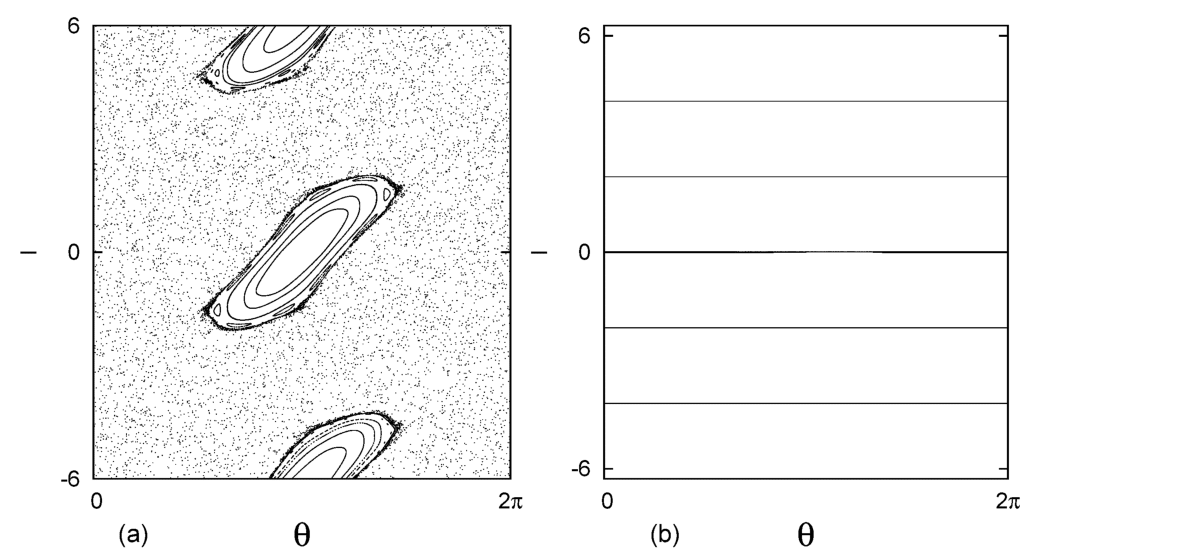
Figure 2: (a) GSM Poincaré section for $\hat{\rho}=3.9$ and $K=8.0$ (point $P_{0}$ in figure 1): no KAM curves are observed. (b) GSM Poincaré section for $\hat{\rho}=5.52$ and $K=8.0$ (point $P_{1}$ in figure 1): KAM curves are restored.

IV.1 Fixed Points

According to Eqs. (30)-(31), the fixed points of the GSNM, $I^{*}=I_{n+1}=I_{n}$ and $\theta^{*}=\theta_{n+1}=\theta_{n}$, satisfy

$$0= bJ_{0}\left(\hat{\rho}\right)\sin(2\pi\theta^{*})$$ (35)

$$m= a\left[\left(1-\frac{\bar{\rho}^{2}}{2}\right)-I^{*}{}^{2}\right]$$ (36)

where $m$ is an integer number. For each $m\in\mathbb{\mathbb{Z}}$, $a\neq 0$, $bJ_{0}\left(\hat{\rho}\right)\neq 0$, and $\bar{\rho}\leq\sqrt{2\left(1-\frac{m}{a}\right)}$, there are four fixed points:

$$P_{\pm}=\left(0,\pm I_{*}\left(\bar{\rho}\right)\right)$$ (37)

$$Q_{\pm}=\left(\frac{1}{2},\pm I_{*}\left(\bar{\rho}\right)\right)$$ (38)

where

$$I_{*}\left(\bar{\rho}\right)=\frac{1}{\sqrt{2}}\sqrt{2\left(1-\frac{m}{a}\right)-\bar{\rho}^{2}}\,.$$ (39)

Note that the $\theta$ coordinate of $P_{\pm}$ and $Q_{\pm}$ does not depend on any parameters. If $\bar{\rho}=\sqrt{2\left(1-\frac{m}{a}\right)}$, the pair of points $\left\{P_{+},P_{-}\right\}$ collide at $\left(0,0\right)$, and $\left\{Q_{+},Q_{-}\right\}$ collide at $\left(\frac{1}{2},0\right)$. Figure 3 shows the $I$-axis position of both pairs for $m=0$ and increasing $\bar{\rho}$. The collision occurs for $\bar{\rho}=\sqrt{2}$. For higher values of $\bar{\rho}$, the fixed points don’t exist.

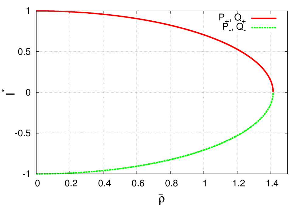
Figure 3: Coordinate $I$ of fixed points for m=0 and increasing $\bar{\rho}$. The fixed points collide at $\bar{\rho}=\sqrt{2}$ and do not exist for $\bar{\rho}>\sqrt{2}$. (Color online)

The stability of a $k$-periodic orbit of a map $M$ is determined by the residue

$$R=\frac{1}{4}\left[2-Tr\left(\prod_{i=0}^{k-1}J\left(\vec{x}_{i}\right)\right)\right]$$ (40)

where $J$ is the Jacobian matrix of $M$, evaluated at the $k$-periodic orbit $\left\{\vec{x}_{i}\right\}_{i=0}^{k-1}$. If $0<R<1$, the periodic orbit is elliptic (stable); if $R<0$ or $R>1$, it is hyperbolic (unstable); and it is parabolic for $R=0$ or $R=1$. Applying formula (40) to the GNSM fixed points in Eqs. (37)-(38) we get

$$R\left(P_{\pm}\right)=R\left(Q_{\mp}\right)=\mp\pi abJ_{0}\left(\hat{\rho}\right)I_{*}\left(\bar{\rho}\right)\,.$$ (41)

The stability of the fixed points $\left\{P_{\pm},Q_{\pm}\right\}$ with $m=0$ can be analyzed using the parameter $\Lambda\left(a,b,\hat{\rho},\bar{\rho}\right)=R\left(P_{-}\right)$. As shown in Fig. 4, depending on the value of $\Lambda$, there are three possible configurations. The symbol “x” denotes an hyperbolic point, and “o” an elliptic point. The points have their stability inverted when $-1<\Lambda<0$ (configuration II), as indicated in Fig. 4-(b). All the fixed points are hyperbolic in configuration III, Fig. 4-(c), which occurs for $\Lambda<-1$ or $\Lambda>1$.

Figure 4: Stability of the fixed points $P_{\pm}$ and $Q_{\pm}$with $m=0$. (Color online)

IV.2 Separatrix reconnection

The location and stability of the fixed points determine the different phase space topologies of the GSNM. These topologies, illustrated in Fig. 5, are characteristic of nontwist maps and are called heteroclinic, separatrix reconnection, and homoclinic del-castillo-1993 . Since the Larmor radius changes the stability of the fixed points, it is expected that it will also change the topology. Figures 5(a)-(c) show the heteroclinic-type, separatrix reconnection, and the homoclinic-type topologies in Poincaré sections of the GSNM for different values of $a$ and $b$, and fixed values of $\hat{\rho}$ and $\bar{\rho}$.

Figure 5: GSNM phase space topologies associated with the fixed points $P_{\pm}$ and $Q_{\pm}$ with $m=0$. In all figures, the Larmor radius is such that $\hat{\rho}=0.05$ and $\bar{\rho}=0.01$.

To determine the condition for separatrix reconnection associated to the fixed points $P_{\pm}$ and $Q_{\pm}$ with $m=0$, we follow Refs. del-castillo-negrete-etal-1996 ; del-castillo-1993 and approximate the GSNM in the vicinity of the fixed points by the Hamiltonian

$$H\left(I,\theta\right)=a\left[I\left(1-\frac{\bar{\rho}^{2}}{2}\right)-\frac{I^{3}}{3}\right]-\frac{b}{2\pi}J_{0}\left(\hat{\rho}\right)\cos\left(2\pi\theta\right)\,.$$ (42)

For $0<\Lambda<1$ (configuration I), separatrix reconnection occurs when $H\left(P_{+}\right)=H\left(Q_{-}\right)$. If $-1<\Lambda<0$ (configuration II), reconnection is observed when $H\left(P_{-}\right)=H\left(Q_{+}\right)$. Combining these two conditions, we obtain the reconnection line

$$a=\frac{3}{4\pi}\sigma\left(\hat{\rho},\bar{\rho}\right)b$$ (43)

with slope:

$$\sigma\left(\hat{\rho},\bar{\rho}\right)=\frac{\left|J_{0}\left(\hat{\rho}\right)\right|}{\left(1-\frac{\bar{\rho}^{2}}{2}\right)^{\frac{3}{2}}}$$ (44)

The reconnection line divides the $a$-$b$ parameter space in two regions: one with heteroclinic-type topology ($\frac{a}{b}>\frac{3}{4\pi}\sigma\left(\hat{\rho},\bar{\rho}\right)$) and another with homoclinic-type topology ($\frac{a}{b}<\frac{3}{4\pi}\sigma\left(\hat{\rho},\bar{\rho}\right)$). The slope of the reconnection line is defined by the angle $\arctan\left[\frac{3}{4\pi}\sigma\left(\hat{\rho},\bar{\rho}\right)\right]$. Figure 6 shows isolines of the angle $\arctan\left[\frac{3}{4\pi}\sigma\left(\hat{\rho},\bar{\rho}\right)\right]$. Keeping $a$ and $b$ fixed, the topology of the phase space remains unchanged if the parameters $\hat{\rho}$ and $\bar{\rho}$ vary over an isoline. As an example, for $a$ and $b$ such that $a=\frac{3}{4\pi}b$ (which corresponds to the reconnection condition in the standard nontwist map del-castillo-1993 ) there is reconnection for any values of $\hat{\rho}$ and $\bar{\rho}$ over the red isoline in Fig. 6. The red isoline crosses the point $\hat{\rho}=\bar{\rho}=0$ where the GNSM reduces to the standard nontwist map. For high (red) values of $\sigma$, the slope of the reconnection line approaches $\frac{\pi}{2}$, and the phase space is characterized by the homoclinic-type topology for a fixed $a$ and almost every value of the parameter $b$. For low (blue) values of $\sigma$, the slope of the reconnection line tends to $0$, and the phase space is characterized by the heteroclinic-type topology for a fixed $b$ and almost every value of the parameter $a$.

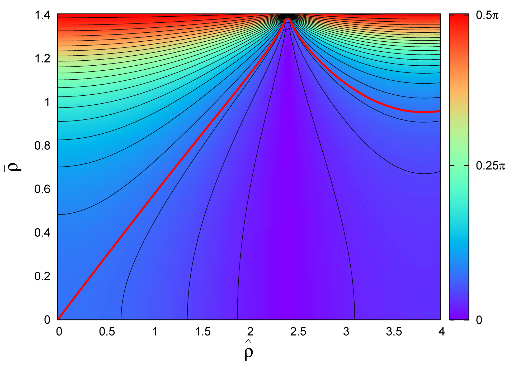
Figure 6: Isolines of $\arctan\left[\frac{3}{4\pi}\sigma\left(\hat{\rho},\bar{\rho}\right)\right]$: varying $\hat{\rho}$ and $\bar{\rho}$ along isolines does not change the topology of the phase space. For high (red) values of $\sigma$, homoclinic-type is observed topology for a fixed $a$ and almost every value of $b$. For low (blue) values of $\sigma$, heteroclinic-type topology is observed for a fixed $b$ and almost every value of $a$. (Color online)

IV.3 Nontwist transport barrier

The transition to global chaos in the GSNM corresponds to the destruction of the nontwist transport barrier (NTB) which is a robust non-chaotic region of KAM curves dividing the phase space. The NTB is robust in the sense that their KAM curves are typically more resilient to perturbation than other KAM curves in the system.

Consider the $3/2$-degrees-of-freedom Hamiltonian system

$$H=H_{0}\left(I\right)+\epsilon V\left(I,\theta,t\right)$$ (45)

where $I$ and $\theta$ are the action-angle variables of the integrable system, $H_{0}$, and the parameter $\epsilon$ controls the strength of the time-periodic perturbation $V$. In this case, the twist (non-degeneracy) condition is

$$\frac{d\Omega}{dI}=\frac{d^{2}H_{0}}{dI^{2}}\neq 0,$$ (46)

for all $I$. If there is at least one critical point for which $d\Omega/dI=0$, the non-degeneracy condition is violated the Hamiltonian in Eq. (45) is nontwist. One of the main properties of these systems is the presence of robust NTBs located at the critical points (maxima or minima) of the frequency profile even in the case when most of the phase space is chaotic del-castillo-1993 . As discussed before, the GSNM can be obtained by integrating the equations of motion of the $3/2$-degrees of freedom Hamiltonian in Eq. (8). This is a nontwist Hamiltonian because the frequency in Eq. (26) has a critical point at $x=0$. Figure 7 shows a Poincaré section of the GSNM with $a=0.354$, $\bar{\rho}=0$, and $bJ_{0}\left(\hat{\rho}\right)=0.8$. As expected, the phase space is characterized predominantly by chaotic orbits (green and red regions), but it has a robust NTB consisting of “belt” of KAM curves (black curves).

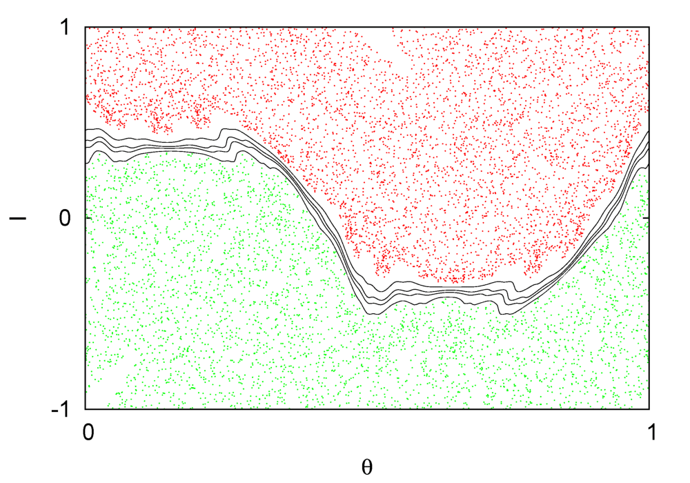
Figure 7: Nontwist transport barrier in the GSNM: robust region of KAM curves (black curves) splitting the phase space in two chaotic regions, indicated by the red and green orbits. (Color online)

IV.4 Breakup Diagrams

Here we study the transition to global chaos in the GSNM, i.e., the destruction of the robust KAM curves that constitute the NTB. It is important to remark that the transition to global chaos in nontwist systems is still an open problem. However, a possible approach to this problem consists of estimating the parameter values, or the critical thresholds, that determine the breakup of the shearless KAM curve. In the absence of a perturbation, the shearless KAM curve is located where the twist condition is violated, and the parameter values for the destruction of the NTB can be estimated from the parameter values that determine the breakup of the shearless curve.

A standard way to determine the parameter values for the destruction of the shearless curve is based on the indicator point (IP) method proposed in Ref.shinohara and used is several works including Refs. Wurm ; Budyansky09 ; del-castillo-martinell2013 . This method consists on finding the parameter values for which the iterations of the indicator point, which defines the indicator point orbit (IPO), are chaotic. If the IPO is quasiperiodic, it traces a shearless KAM curve. When the IPO is chaotic, the shearless curve is broken. In nontwist maps with special symmetries, like the ones studied here, the indicator points can be easily found by computing the fixed points of the reversing symmetry group transformations. Further details can be found in Ref. Petrisor . Following a procedure similar to the one in Ref. Wurm , we obtained the following IPs for the gyro-averaged standard nontwist map

$$z_{0}^{1}=\left(\frac{1}{4},\frac{bJ_{0}\left(\hat{\rho}\right)}{2}\right)\quad z_{0}^{2}=\left(\frac{3}{4},-\frac{bJ_{0}\left(\hat{\rho}\right)}{2}\right)\\$$ (47)

$$z_{1}^{1}=\left(\frac{a}{2}\left[1-\frac{\bar{\rho}^{2}}{2}\right]+\frac{1}{4}\quad{\rm mod}\quad 1,\quad 0\right)\qquad z_{1}^{2}=\left(\frac{a}{2}\left[1-\frac{\bar{\rho}^{2}}{2}\right]+\frac{3}{4}\quad{\rm mod}\quad 1,0\right)$$ (48)

Once the IPs are found, the next step is to obtain the critical thresholds using an appropriate criterion to determine if the IPO is chaotic. Our criterion is based on the technique proposed in Altmann , which considers the recurrence properties of the IPO in conjunction with Slater’s Theorem Slater . Recurrence properties and their relation to the Slater’s Theorem were also discussed in Zou . In Ref. Abud , the technique described in Ref. Altmann was used to study the breakup of the shearless curve in the nontwist standard map. The Slater’s Theorem states that, for any quasiperiodic motion on the circle, there are at most three different recurrences, or return times, in any connected interval. Although this theorem was originally formulated for circle maps, it can also be applied to two-dimensional systems, once the dynamics on a KAM curve is mapped to a quasiperiodic rotation on a circle Altmann . The recurrence time is defined as the number of iterations that an orbit takes to return to a neighborhood of a point. Our procedure to characterize the dynamics of an indicator point orbit of the GSNM is the following: with any one of the indicator points as the initial condition, we compute the orbit for $N$ iterations and choose the point of the orbit which has the maximum number of different recurrence times. If there are more than three different recurrence times, we conclude that the orbit is chaotic and the corresponding KAM curve is destroyed. More precisely, the procedure consists of the following steps:

• Compute the orbit $O=\{u_{k}\}_{k=0}^{N}$ with initial condition $u_{0}=z_{1}^{1}$, where $N$ is the number of iterations.

• Construct the recurrence matrix :

  $$R_{ij}=\Theta(\epsilon-\left\|u_{i}-u_{j}\right\|)$$ (49)

  where $i,j\in\left\{0,...,N\right\}$, $u_{i},u_{j}\in O$, $\Theta$ is the Heaviside function, and $\epsilon$ is a parameter defining the size of the neighborhood. If the distance between $u_{i}$ and $u_{j}$, given by the norm $\left\|u_{i}-u_{j}\right\|$, is less than $\epsilon$, $R_{ij}=1$; otherwise, $R_{ij}=0$.

• Define the recurrence time as $\tau_{ij}=\left|i-j\right|$ for $i\neq j$ and $R_{ij}=1$. That is, the recurrence time is $\tau_{ij}$ if the orbit crosses the neighborhood of $u_{j}$ at the $i$-th iteration. For each point $u_{j}$, compute the set of different recurrences $S^{(j)}_{R}=\cup_{i=0,i\neq j}^{N}\left\{\tau_{ij}\right\}$.

• Determine the maximum number of different recurrence times:

  $$n_{R}=max\left\{n\left(S^{(j)}_{R}\right)\right\}_{j=0}^{N}$$ (50)

  where $n$ is the number of recurrence times belonging to $S^{(j)}_{R}$, and use the Slater’s Theorem to conclude that the orbit $O$ is chaotic if $n_{R}>3$.

For $n_{R}\leq 3$, the characterization of the dynamics using the Slater’s Theorem is inconclusive because the orbit might be periodic, quasiperiodic or even chaotic. In this case, the number of iterations, $N$, can be increased to explore if $n_{R}$ increases beyond $3$. If the condition $n_{R}\leq 3$ still persists and no change in $n_{R}$ is observed, the orbit is deemed periodic if $n_{R}=1$ and quasiperiodic if $n_{R}=3$. The case $n_{R}=2$ requires a more careful analysis with higher values $N$. Increasing $N$, $n_{R}$ stabilizes in $3$, indicating quasiperiodic dynamics, or assumes values greater than $3$, which is the case for chaotic dynamics. Although rigorous criteria for the case $n_{R}\leq 3$ are lacking, the numerical results in Refs. Altmann ; Zou support the use of recurrences in conjunction with Slater’s theorem as a computationally efficient diagnostic to identify chaotic orbits.

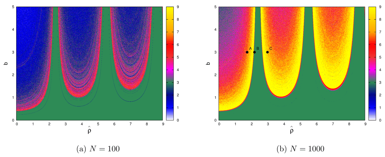
Figure 8: GSNM breakup diagrams for $\hat{\rho}$ versus $b$, with $\bar{\rho}=0$, and $a=0.1$. For each point $(\hat{\rho},b)$ in the diagram, the IPO and the correspondent $n_{R}$ are computed with $\epsilon=0.1$. The color pallet indicates the value of $n_{R}$. The breakup of the shearless curve can be detected in the points where $n_{R}>3$. The IPO is quasiperiodic in the green region ($n_{R}=3$), which corresponds to low effective perturbation $b_{ef}$, i.e., low $b$ or $\hat{\rho}$ near a zero of $J_{0}$. (Color online)

We now apply this diagnostic to compute breakup diagrams for the GSNM showing regions in parameter space where the shearless curve is broken. The diagrams were constructed by computing the recurrences of IPOs for $\epsilon=0.1$, and two different number of iterations, $N=100$ and $N=1000$. Since the GSNM has four free parameters only two parameters were varied at a time while the others were kept constant. Our first example is presented in Fig. 8 where we fixed $a=0.1$, $\bar{\rho}=0$ (which corresponds to the limit $\rho\ll L$), and plotted the values of $n_{r}$ on a $1000\times 1000$ grid in the $(\hat{\rho},b)$ space. The main difference between $N=100$ and $N=1000$ is observed in points with $n_{R}=2$, but even for a relatively small number of iterations it is possible to identify the breakup of the shearless curve in domains where $n_{R}>3$. These domains have points plotted with magenta, red, and yellow colors. Green points ($n_{R}=3$) are concentrated in domains with low effective perturbation $b_{ef}$, which means small $b$ or $\hat{\rho}$ close to a zero of the zero-order Bessel function. For parameter values outside the green region (e.g., points $A$ and $C$ in Fig. 8) the IPO is chaotic, and, as shown in Fig. 9, the shearless curve is destroyed. For $\hat{\rho}$ values near a zero of $J_{0}$ (e.g., point $B$ of Fig. 8), the shearless KAM curve is restored as shown by the red orbit in Fig. 9.

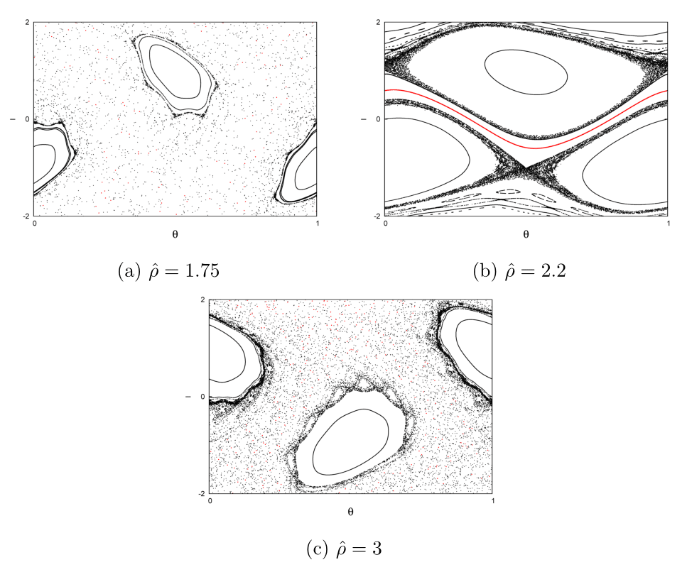
Figure 9: Restoration of shearless KAM curve (identified through a quasiperiodic IPO shown in red) for $\hat{\rho}$ values near the zeros of $J_{0}$ and $a=0.1$, $b=3$, and $\bar{\rho}=0$. Panels (a), (b) and (c) correspond to parameter values A, B, and C indicated in Fig. 8. As expected, for $\hat{\rho}=2.2$, which is near a zero of the Bessel function, the effective perturbation parameter is small and the shearless curve is restored. (Color online)

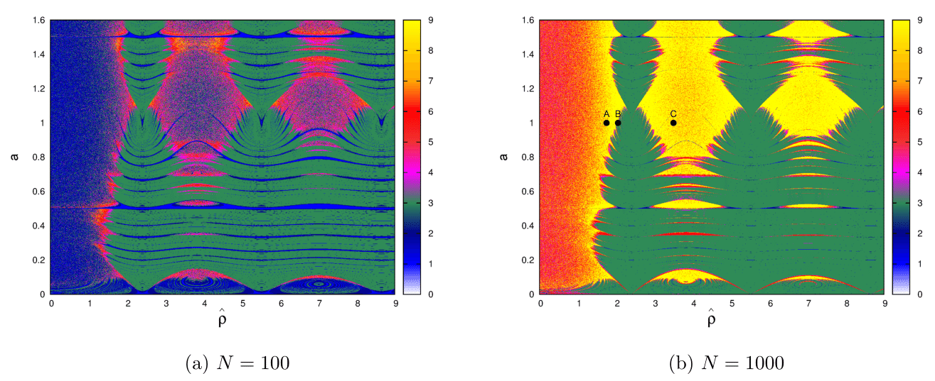
Figure 10: GSNM breakup diagrams for $\hat{\rho}$ versus $a$, with $\bar{\rho}=0$ and $b=1.5$. Neighborhood size: $\epsilon=0.1$. Green points, corresponding to quasiperiodic dynamics, are concentrated near the zeros of $J_{0}$ and in domains with low $a$. (Color online)

Breakup diagrams with varying $a$ and $\hat{\rho}$ are shown in Fig. 10. The number of iterations used to construct the first diagram was $N=100$. In the second diagram, the number of iterations was increased to $N=1000$. As before, regions where $n_{R}=3$, which are indicators of non-chaotic dynamics, are concentrated near the zeros of $J_{0}$. A high occurrence of points with $n_{R}=3$ is also observed in regions with low $a$. When the number of iterations is increased from $N=100$ to $N=1000$, it s observed that the main geometric features remain the same, although several points with $n_{R}=1$ and $n_{R}=2$ transition to $n_{R}>3$. Poincaré sections for parameters corresponding to points $A$, $B$, and $C$ in Fig. 10 are showed in Fig. 11a-c. As expected, the shearless KAM curve is broken at points $A$ and $C$, and restored at point $B$.

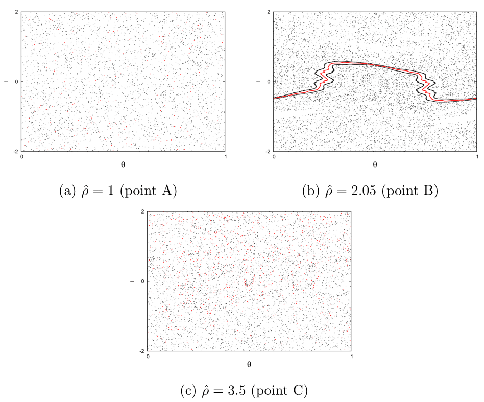
Figure 11: Poincaré sections of the GSNM map for parameter values corresponding to points A, B and C, in Fig. 8, and $a=1$; $b=1.5$; $\bar{\rho}=0$. Consistent with Fig. 8-(b), the shearless curve is restored for $\hat{\rho}=2.05$. (Color online)

Additional examples of breakup diagrams are presented in Figs. 12 (a)-(d). The parameters are the same as those in Figs. 8-(b) and 10-(b), but the value of the fixed parameter $\bar{\rho}$ is higher. Comparing Figs. 12 (a)-(b) to 8-(b), it is observed that increasing $\bar{\rho}$ leads to an increase in the number of points with $n_{R}=3$ and to the robustness of the shearless KAM curve. As shown in Figs. 12 (c)-(d), the distribution of points with $n_{R}=3$ changes when $\bar{\rho}$ increases, resulting in different critical thresholds but with no significant suppression of green points. Red and yellow points disappear in certain regions and reappear in others, as can be seen by comparing Figs. 10-(b), 12-(c) and 12-(d).

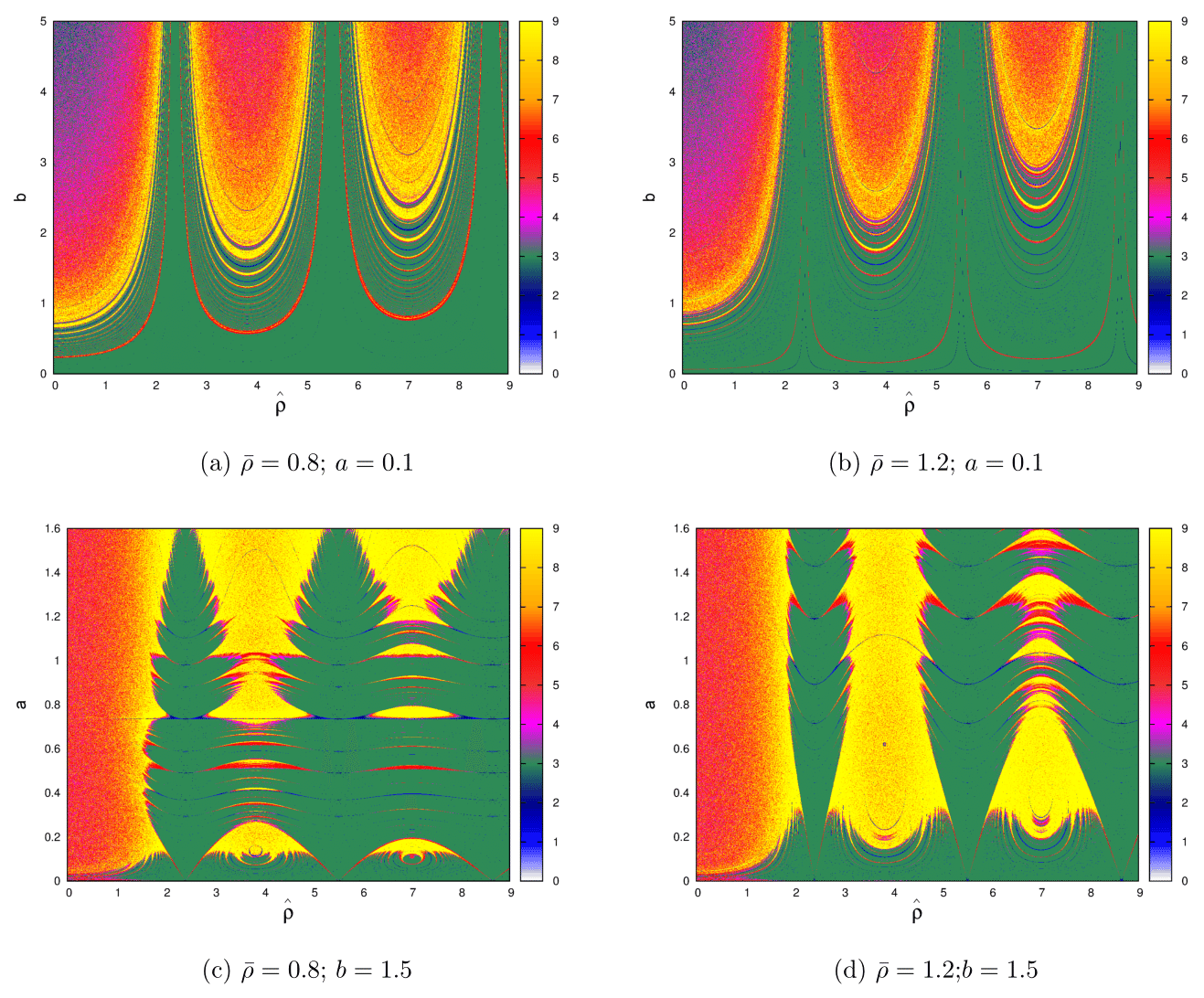
Figure 12: Dependence of robustness of shearless curve on $\bar{\rho}$. As shown in (a) and (b), the robustness of the shearless KAM increases when $\bar{\rho}$ increases with fixed $a=0.1$. On the other hand, as shown in (c) and (d), a different behavior is observed for fixed $b=1.5$. In all diagrams, $N=1000$ and $\epsilon=0.1$. (Color online)

Summarizing, in this section we used a computational technique based on the recurrence properties of the IPO to estimate the critical parameter values for the breakup the shearless KAM curve. In particular, we computed breakup diagrams to understand the role of finite Larmor radius effects on the destruction and formation of shearless KAM curves. It was observed that when $\hat{\rho}$ is close to a zero of $J_{0}$, the shearless curve becomes more robust to perturbation in $b$. This is because, near the zeros of $J_{0}$, the GSNM’s Hamiltonian is effectively integrable. In particular, as $\hat{\rho}$ approaches a zero of $J_{0}$, the shearless curve, and the KAM curves that make up the nontwist transport barrier, are restored. The robustness of the shearless curve and the critical thresholds are also modified by increasing $\bar{\rho}$.

V Gyro-averaged quartic nontwist map

In this section, we propose another area-preserving map, the gyro-averaged quartic nontwist map (GQNM). A key property of the GQNM is that it exhibits a zonal flow bifurcation, similar to the one observed in the nontwist Hamiltonian system of Ref. del-castillo-martinell2013 . The Hamiltonian system in Ref. del-castillo-martinell2013 is a drift-wave model of the ${\bf E}\times{\bf B}$ transport with FLR effects, and the zonal flow bifurcation corresponds to a bifurcation of the maximum of the ${\bf E}\times{\bf B}$ zonal flow velocity when the Larmor radius increases.

As in the previous maps, the GQNM is obtained from the gyro-averaged drift wave map in Eqs. (11) and (12). The equilibrium potential similar to the one proposed in Ref. del-castillo-martinell2013

$$\phi_{0}(x)=\alpha\tanh\left(\frac{x}{L}\right),$$ (51)

where $\alpha$ and $L$ are dimensional constants. Applying the gyro-average operation (4) to (51) gives

$$\langle H_{0}(x)\rangle_{\varphi}=\frac{\alpha}{2\pi B_{0}}\int_{0}^{2\pi}\tanh\left(\frac{x}{L}+\frac{\rho}{L}\cos\varphi\right)\,d\varphi\,,$$ (52)

and from Eq. (13) we get the nonlinear frequency

$$\Omega\left(I\right)=\frac{\alpha}{2\pi LB_{0}}\int_{0}^{2\pi}\mathrm{sech}^{2}\left(I+\bar{\rho}\cos\varphi\right)\,d\varphi$$ (53)

where $I=x/L$, and $\bar{\rho}=\rho/L$. The zonal flow bifurcation results from a bifurcation of the critical point of the frequency profile. To analyze it in a simple setting, consider the Taylor series approximation of (53) for small values of $|I|$ and $\bar{\rho}$,

$$\Omega\left(I\right)\approx\frac{\alpha}{LB_{0}}\left(1-I^{2}\right)\left\{1-\bar{\rho}^{2}\left[\frac{3}{2}\left(1-I^{2}\right)-1\right]\right\}\,.$$ (54)

Figure 13 shows the frequency profile in Eq. (54) for different values of $\bar{\rho}$. For $\bar{\rho}=0$, there is only one critical point, $\Omega^{\prime}=0$, which corresponds to a maximum at $I=0$. Increasing $\bar{\rho}$ leads to an increase of the profile’s “flatness” and eventually to a transition in which the maximum bifurcates into a minimum and two maxima. The bifurcation threshold $\bar{\rho}_{b}$ can be determined from the condition,

$$\frac{\partial^{2}\Omega}{\partial I^{2}}\bigg{|}_{I=0,\;\bar{\rho}=\bar{\rho}_{b}}=0\,,$$ (55)

which for Eq. (54) gives

$$\bar{\rho}_{b}=1/\sqrt{2}.$$ (56)

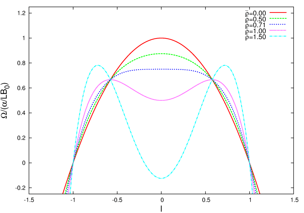
Figure 13: Bifurcation of critical points in the frequency profile (54) (Color online)

Defining $I_{n}=x_{n}/L$, $\theta_{n}=ky_{n}/2\pi$, and $\hat{\rho}=k\rho$, and using Eq. (54), we get from Eqs. (11) and (12), the GQNM

$$I_{n+1}= I_{n}+bJ_{0}\left(\hat{\rho}\right)\sin\left(2\pi\theta_{n}\right)$$ (57)

$$\theta_{n+1}= \theta_{n}+a\left(1-I_{n+1}^{2}\right)\left\{1-\bar{\rho}^{2}\left[\frac{3}{2}\left(1-I_{n+1}^{2}\right)-1\right]\right\},\quad{\rm mod}\quad 1$$ (58)

where $a=k\alpha/\omega_{0}LB_{0}$, and the perturbation parameter is $b=2\pi aA/\alpha$. As in the previous maps, an effective perturbation parameter can be defined as $b_{ef}=bJ_{0}\left(\hat{\rho}\right)$. Like the GSNM, the GQNM reduces to the standard nontwist map for $\hat{\rho}=\bar{\rho}=0$. In what follows, we discuss FLR effects on the GQNM’s fixed points and nontwist transport barriers.

V.1 Fixed Points and nontwist transport barriers

The fixed points $\left(\theta^{*},I^{*}\right)$ of the GQNM satisfy

$$0= bJ_{0}\left(\hat{\rho}\right)\sin\left(2\pi\theta^{*}\right)$$ (59)

$$m= a\left(1-I^{*2}\right)\left\{1-\bar{\rho}^{2}\left[\frac{3}{2}\left(1-I^{*2}\right)-1\right]\right\},\quad m\in\mathbb{\mathbb{Z}}\,.$$ (60)

For $m=0$, $a\neq 0$, and $bJ_{0}\left(\hat{\rho}\right)\neq 0$, there are four fixed points independently of the value of $\rho$,

$$P_{1}^{\pm}=\left(0,\pm 1\right),\qquad Q_{1}^{\pm}=\left(\frac{1}{2},\pm 1\right)\,.$$ (61)

If $\bar{\rho}\geq 2\bar{\rho}_{b}=\sqrt{2}$, there is an additional set of fixed points,

$$P_{2}^{\pm}=\left(0,\pm h\left(\bar{\rho}\right)\right)\qquad Q_{2}^{\pm}=\left(\frac{1}{2},\pm h\left(\bar{\rho}\right)\right)\,,$$ (62)

where

$$h\left(\bar{\rho}\right)=\sqrt{\frac{\bar{\rho}^{2}-2}{3\bar{\rho}^{2}}}\,.$$ (63)

Figure 14 shows the $I$ coordinates of the fixed points with $m=0$. $P_{1}^{\pm}$ and $Q_{1}^{\pm}$ exist for all $\bar{\rho}\geq 0$ and are always located at $I=\pm 1$. $P_{2}^{\pm}$ and $Q_{2}^{\pm}$ only exist for $\bar{\rho}\geq 2\bar{\rho}_{b}=\sqrt{2}$ and their positions in the $I$ axis are determined by the function $h\left(\bar{\rho}\right)$, which satisfies $0\leq h\left(\bar{\rho}\right)<\frac{1}{\sqrt{3}}$.

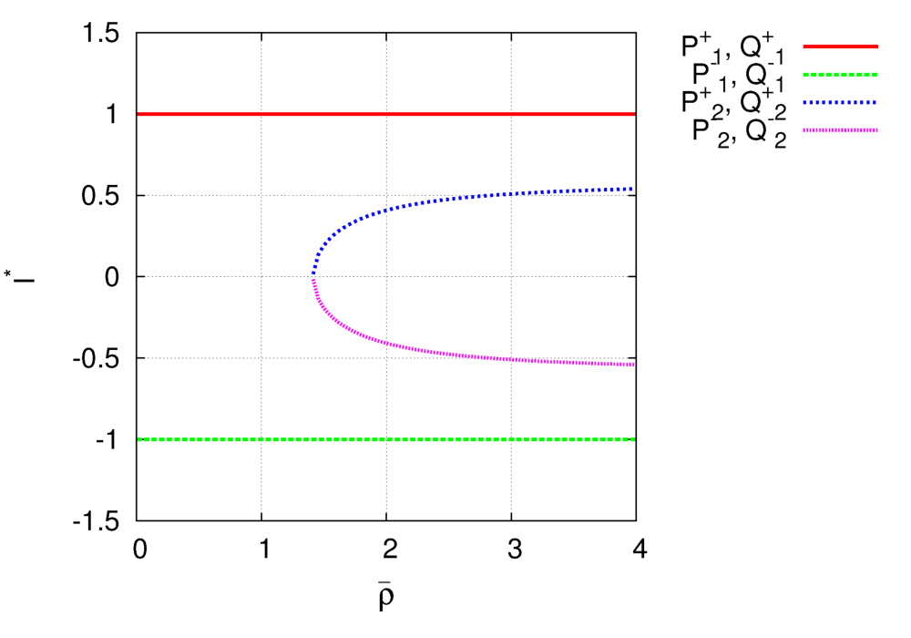
Figure 14: $I$ coordinates of fixed points with $m=0$ as function of $\hat{\rho}$. The set $\left\{P_{1}^{\pm},Q_{1}^{\pm}\right\}$ exists for all values of $\bar{\rho}$. The set $\left\{P_{2}^{\pm},Q_{2}^{\pm}\right\}$ only exists for $\bar{\rho}\geq 2\bar{\rho}_{b}=\sqrt{2}$. (Color online)

The stability of the fixed points $\left\{P_{1}^{\pm},Q_{1}^{\pm},P_{2}^{\pm},Q_{2}^{\pm}\right\}$ can be analyzed by evaluating the Green’s residue in Eq. (40)

$$R\left(P_{1}^{\pm}\right) =-R\left(Q_{1}^{\pm}\right)=\mp\Lambda\left(a,b,\hat{\rho},\bar{\rho}\right)$$ (64)

$$R\left(P_{2}^{\pm}\right) =-R\left(Q_{2}^{\pm}\right)=\pm h\left(\bar{\rho}\right)\Lambda\left(a,b,\hat{\rho},\bar{\rho}\right)$$ (65)

where

$$\Lambda=\pi abJ_{0}\left(\hat{\rho}\right)\left(1+\bar{\rho}^{2}\right)\,.$$ (66)

As shown in Fig. 15, depending on the value of $\Lambda$, there are five possible stability configurations. The number of elliptic fixed points reduces when $\Lambda$ increases, and for $\left|\Lambda\right|>\frac{1}{h\left(\bar{\rho}\right)}$ all the fixed points are hyperbolic. In general, the first points to lose stability are the outer ones. Note that as $\bar{\rho}$ approaches the zonal bifurcation threshold, $1/h(\bar{\rho})$ diverges, and the range of the configurations III and IV increases.

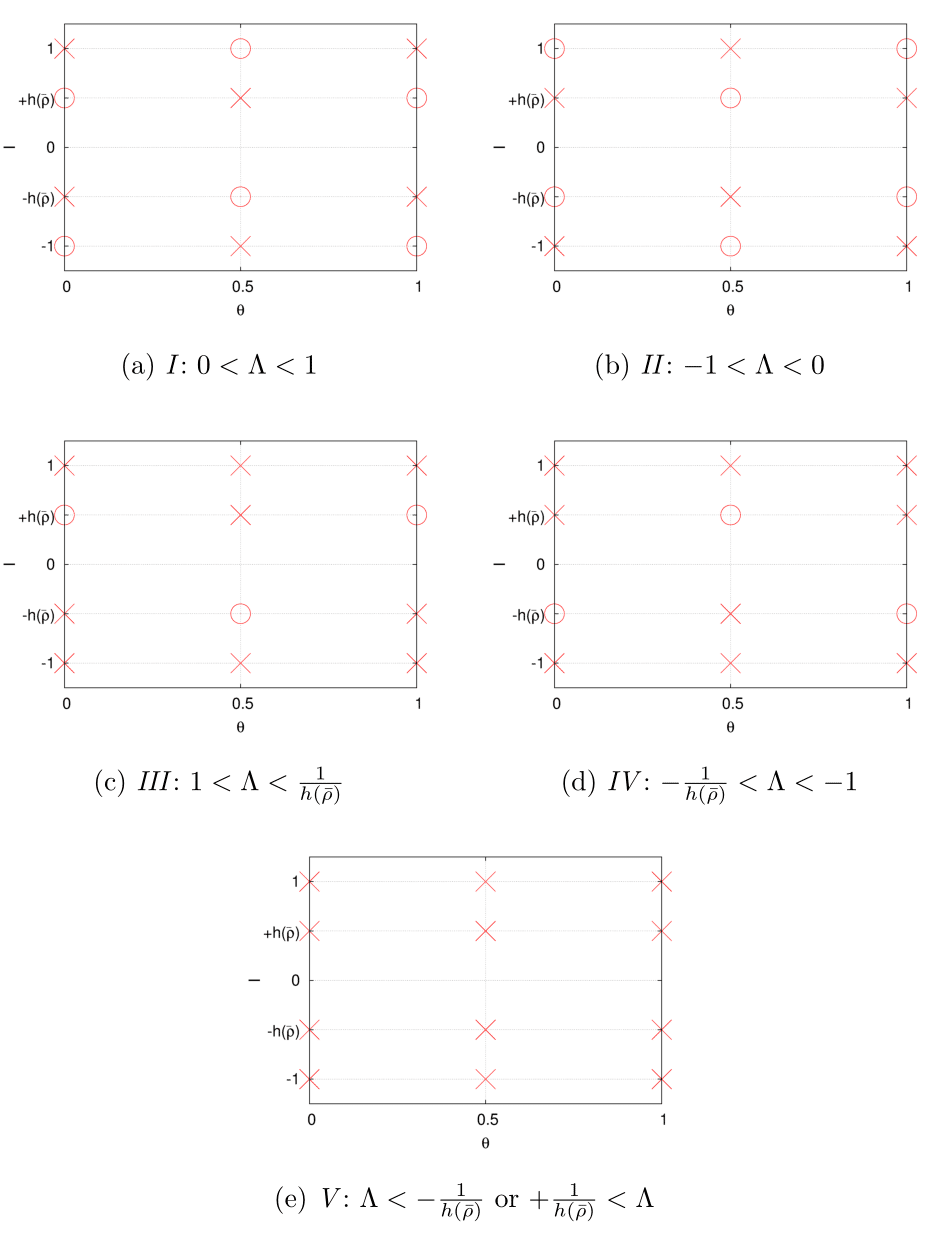
Figure 15: Depending on the value of $\Lambda$, there are five possible configurations characterizing the stability of the period-one fixed points $\left\{P_{1}^{\pm},Q_{1}^{\pm},P_{2}^{\pm},Q_{2}^{\pm}\right\}$ in the GQNM. (Color online)

An important consequence of the zonal flow bifurcation is the occurrence of nontwist barrier bifurcations. In particular, for $\bar{\rho}\lesssim\bar{\rho}_{b}$, only one region with robust KAM curves is present (Fig. 16)-(a), but for $\bar{\rho}>\bar{\rho}_{b}$ (Fig. 16)-(b) two additional NTBs appear. The outer NTBs are separated from the central one by two regions of confined chaotic orbits.

Figure 16: (a) One NTB for $\bar{\rho}\lesssim\bar{\rho}_{b}$. (b) After the zonal flow bifurcation, three NTBs can be observed. Parameters: $a=0.5$; $b=1.35$; $\hat{\rho}=2.8$.

V.2 Robustness of the central shearless curve

Our interest in studying the robustness of KAM curves as function of $b$ resides on the fact that this parameter is proportional to the amplitude of the drift waves. For very small Larmor radius (or in the absence of FLR corrections), high amplitude values can easily destroy all KAM curves. However, this is not always the case when FLR effects are taken into account. In particular, like in the GSNM (see Sec. IV.3), the robustness of the GQNM’s shearless curve is significantly increased for $\hat{\rho}$ near a zero of $J_{0}$.

Figures 17(a)-(d) show breakup diagrams for the shearless KAM curve in the GQNM as function of $b$ and $\bar{\rho}$. In all cases, $b_{ef}$ is small, because the values of $\hat{\rho}$ are close to the zeros of $J_{0}$. Under this condition, and when $\bar{\rho}$ is close to the zonal flow bifurcation threshold $\bar{\rho}_{b}$ in Eq. (56), a significant increasing of the robustness of the shearless curve is observed. For $\bar{\rho}<\bar{\rho}_{b}$, higher values of $b$ are required for breakup as $\bar{\rho}$ approaches $\bar{\rho}_{b}$, and for $\bar{\rho}>\bar{\rho}_{b}$, the robustness is reduced as $\bar{\rho}$ increases. That is, the robustness of the central NTB increases for $\hat{\rho}$ close to the zeros of $J_{0}$, and for $\bar{\rho}$ close to $\bar{\rho}_{b}$.

It is interesting to note that, in the neighborhood of the $I=0$ shearless point, the degree of “flatness” of the frequency’s profile has a similar behavior. In particular, like the robustness of the central shearless curve, the degree of “flatness” (measured by $\left|\Omega^{\prime\prime}(0)\right|$) is higher near the bifurcation threshold, but it becomes smaller elsewhere. These results provide support to the conclusion that the robustness of NTBs in nontwist maps depends on the flatness of the frequency profile at the maximum or minimum (critical points), and that, for small perturbation, the robustness increases with the degree of flatness.

Figure 17: For small $b_{ef}$ values, the robustness of the central shearless curve (and, thus, also of the central NTB) increases with the degree of flatness of the frequency’s profile around the critical point. The flatness can be controlled by the parameter $\bar{\rho}$ and becomes higher when $\bar{\rho}$ is close to the zonal flow bifurcation threshold $\bar{\rho}_{b}$ (shown with the solid black vertical line). The values of $b_{ef}$ are made small by setting $\hat{\rho}$ close to the zeros of $J_{0}$. The first four positive zeros are approximately given by: $\rho_{1}=2.40$; $\rho_{2}=5.52$; $\rho_{3}=8.65$; $\rho_{4}=11.79$. (Color online)

The understanding of the role of the shear and the flatness of the frequency on the robustness of KAM curves is still an open problem. Among the first works addressing the role of shear is Ref. finn_1975 where it was analytically and numerically shown that high shear reduces the strength of the perturbation required to break KAM surfaces. However this work limited attention to monotonic frequencies with non-vanishing shear (i.e., twist systems) and did not address the breakup of shearless KAM curves. The robustness of NTBs is also related to the strong KAM stability in nontwist maps Rypina . According to the resonant overlap criterion chirikov79 , tori located between resonances break when the resonances overlap. Thus, one expects tori to be more resilient when the resonances’ widths are small. As shown in Ref. Rypina , in $3/2$-degrees-of-freedom nontwist Hamiltonian systems, the width, $\delta\Omega$, of second-order degenerate resonances scales as

$$\delta\Omega\sim\left[\epsilon\left|\Omega^{\prime\prime}(I_{0})\right|\right]^{2/3}\,,$$ (67)

where $\epsilon$ is the amplitude of the perturbation, and $I_{0}$ is such that

$$\Omega^{\prime}(I_{0})=0\qquad\Omega^{\prime\prime}(I_{0})\neq 0\,,$$ (68)

which according to Eq. (46) corresponds to the point where the twist condition is violated. When the system is slightly perturbed, second-order degenerate resonances appear in the neighborhood of the shearless curve, and their overlap leads to the break up of the shearless curve.

The central shearless curve of the GQNM is associated to the critical point $I_{0}=0$ where the frequency in Eq. (54) satisfies (68) for $\bar{\rho}\neq\bar{\rho}_{b}$. Thus, in the Hamiltonian system from which the GQNM is derived, second-order degenerate resonances might appear near the central shearless curve, and according to Eqs. (67) and (55), the width of these resonances scales as

$$\lim_{\bar{\rho}\to\bar{\rho}_{b}}\delta\Omega=0\,,$$ (69)

because $\left|\Omega^{\prime\prime}(I_{0})\right|$ vanishes for $\bar{\rho}=\bar{\rho}_{b}$. Small values of $\left|\Omega^{\prime\prime}(I_{0})\right|$ result in small degenerate resonance widths and a more robust central shearless curve. As $\left|\Omega^{\prime\prime}(I_{0})\right|$ is directly related to the flatness of the frequency’s profile at $I_{0}$, Eq. (67) is consistent with the results Figs. 17(a)-(b) and supports the conjecture relating the robustness of shearless curves to the flatness of the frequency at the degenerate points. Similar arguments can be applied to interpret the results in Ref. Firpo2009 where a study of the effect of the flatness of the $q$-profile on the robustness of NTBs was presented.

VI Summary and Conclusions

In this paper we studied finite Larmor radius effects on discrete models of $\vec{E}\times\vec{B}$ chaotic transport of test charged particles. The models are area-preserving Hamiltonian maps that assume an electrostatic potential consisting of the superposition of an equilibrium radial electrostatic field and a perturbation with a broad spectrum of drift waves. FLR effects were included by gyro-averaging the electrostatic potential and the maps were constructed from the integration of the resulting gyro-averaged $\vec{E}\times\vec{B}$ Hamiltonian system.

We constructed and studied three maps: the gyro-averaged standard map (GSM), the gyro-averaged standard nontwist map (GSNM), and the gyro-averaged quartic nontwist map (GQNM). In the GSM, the frequency, i.e. the gyro-averaged $\vec{E}\times\vec{B}$ zonal flow velocity, has a monotonic radial profile and the map satisfies the twist condition. In the GSNM and GQNM cases the frequency is non-monotonic and as a result the maps are nontwist. Non-monotonic frequencies have degenerate points (i.e., points where the frequency is maximum or minimum), and in the vicinity of these points robust nontwist transport barriers (NTBs) tend to form.

Typically, in area preserving maps, increasing the perturbation increases the chaos in the phase space. However, even for large perturbations, FLR effects can suppress chaos and restore broken KAM curves. The breakup diagrams provide the critical thresholds for the breakup of the shearless curve which is one of the robust KAM curves that constitute the NTB. To determine the breakup of the shearless curve we used an efficient and accurate method based on the maximum number of different recurrence times. We showed that a relatively low number of iterations is sufficient to determine the main features of the breakup diagrams. Although in general chaos is suppressed when the Larmor radius is close to zeros of the zero-order Bessel function, the breakup diagrams exhibit a highly nontrivial fractal-like dependence on the Larmor radius and the other parameters of the map.

We also studied the role of the Larmor radius on the topology of the phase space and on bifurcations of the ${\bf E}\times{\bf B}$ zonal flow. In particular, we showed that the GSNM exhibits FLR dependent separatrix reconnection and obtained a formula determining the threshold for bifurcation from homoclinic to heteroclinic topologies as function of the Larmor radius. We also found that in the GQNM there is a critical value of the Larmor radius for which the maximum of the ${\bf E}\times{\bf B}$ zonal flow bifurcates into a minimum and two maxima. These zonal flow bifurcations create additional shearless curves that play a highly nontrivial role on transport.

Motivated by the key role that periodic orbits play on transport we presented a detailed study of FLR effects on the location and stability of period-one orbits. In the GSNM there are four period-one orbits and, depending on the value of the Larmor radius, there are three possible stability configurations. In the GQNM the situation is more complex due to the existence of zonal flow bifurcations. In particular, there can be up to eight period-one fixed points, four of which only exist for Larmor radii greater than a critical threshold. In this case, depending on the value of the Larmor radius, there are five stability configurations. It was found that the elliptic fixed points created by varying the Larmor radius are strongly stable. The presence of elliptic points results in the formation of islands that can trap orbits in the phase space.

An important consequence of zonal flow bifurcations is the occurrence of up to three nontwist transport barriers. We focused on the central NTB and analyzed the robustness of the shearless curve using breakup diagrams. The results showed that the robustness of the central shearless curve significantly increases when the Larmor radius is close to the critical threshold for the zonal flow bifurcation. Based on this we argued that, in agreement with previous works, the “flatness” of the frequency profile at the critical point is directly associated with the robustness of the central shearless curve.

VII Acknowledgments

This work was made possible through financial support from the Brazilian research agency FAPESP under grant 2013/00483-1. The authors would like to acknowledge Celso V. Abud for valuable discussions. DdCN was sponsored by the Office of Fusion Energy Sciences of the US Department of Energy at Oak Ridge National Laboratory, managed by UT-Battelle, LLC, for the U.S. Department of Energy under contract DE-AC05-00OR22725. JDF gratefully acknowledges the hospitality of the Oak Ridge National Laboratory where part of work was conducted.

References

- (1) R. G. Kleva, and J. F. Drake, Phys. Fluids 27, 1686 (1984).
- (2) M. Pettini, A. Vulpiani, et al. Phys. Rev. A 38, 344 (1988)
- (3) F. A. Marcus, I. L. Caldas, Z. O Guimaraes Filho, P. J. Morrison, W. Horton, Y. K Kuznetsov and I. L. Nascimento, Phys. Plasmas 15, 112304 (2008).
- (4) D. del-Castillo-Negrete, Phys. Plasmas 7, 1702 (2000).
- (5) G. Manfredi and R. O. Dendy, Phys. Rev. Lett., 76, 4360, (1996).
- (6) J.J. Martinell and D. del-Castillo-Negrete, Phys. Plasmas 20, 022303 (2013).
- (7) S.V. Annibaldi, G. Manfredi, and R. O. Dendy, Phys. Plasmas 9, 791 (2002).
- (8) G. Manfredi and R. Dendy, Phys. Plasmas 4, 628 (1997).
- (9) K. Gustafson, D. del-Castillo-Negrete and W. Dorland, Phys. Plasmas 16, 102309 (2008).
- (10) D. del-Castillo-Negrete and J.J. Martinell, Commun. Nonlinear Sci. Numer. Simulat. 17, 2031 (2012).
- (11) W. Horton, Plasma Phys. Controlled Fusion 27, 9 (1985).
- (12) W. W. Lee, J. Comp. Phys 72, 243 (1987).
- (13) G. A. Oda and I. L. Caldas, Chaos, Solitons and Fractals, 5 15 (1995).
- (14) R. Balescu, Phys. Rev. E 58, 3 (1998).
- (15) D. del-Castillo-Negrete and P. J. Morrison, Bull. Am. Phys. Soc., Series II, 37, 1543 (1992)
- (16) L. Nasi and M.-C. Firpo, Plasma Physics and Controlled Fusion, 51, 045006 (2009).
- (17) D. del-Castillo-Negrete and P. J. Morrison, Phys. Fluids A 5, 948 (1993)
- (18) F. J. Beron-Vera, M. J. Olascoaga, M. G. Brown MG, et al. Chaos 20, 017514 (2010).
- (19) M. V. Budyansky, M. Yu. Uleysky, and S. V. Prants, Phys. Rev. E, 79, 056215 (2009).
- (20) D. del-Castillo-Negrete, J. M. Greene, and P. J. Morrison, Physica D 91, 1 (1996).
- (21) I.I Rypina, M. G. Brown, et al. Phys. Rev. Lett. 98, 104102 (2007).
- (22) J. S. E. Portela, I. L. Caldas et al. International Journal of Bifurcation and Chaos in Applied Sciences and Engineering, 17, 1589, (2007).
- (23) J. D. Szezech, I. L. Caldas, et al. Chaos: An Interdisciplinary Journal of Nonlinear Science, 19, 043108 (2009).
- (24) I.L. Caldas, R.L. Viana et al. Commun. Nonlinear Sci. Numer. Simulat. 17, 2021 (2011)
- (25) A. Delshams and R. de-la-Llave, SIAM J. Math. Anal., 31, 1235 (2000)
- (26) E. G. Altmann, G. Cristadoro, and D. Pazó, Phys. Rev. E, 73, 056201 (2006).
- (27) Y. Zou, D. Pazó, et al. Phys. Rev. E, 76, 016210 (2007).
- (28) C.V. Abud, PhD Thesis, University of São Paulo, (2013).
- (29) D.R Nicholson, “Introduction to Plasma Theory”. John Wiley and Sons, Inc. New York, 1983.
- (30) W. Horton, H.-B. Park, J.-M. Kwon, D. Strozzi, P. J. Morrison, and D.-I. Choi, Phys. Plasmas 5, 11 (1998).
- (31) B. V. Chirikov, Phys. Rep., 52, 263, (1979).
- (32) J. B. Taylor, Culham Lab. Prog. Report CLM-PR-12, (1969).
- (33) J.D. Meiss, Rev. Mod. Phys. 64, 3 (1992).
- (34) J.M Greene, J. Math. Phys. 20, 1183 (1979)
- (35) S. Shinohara and Y. Aizawa, Prog. Theor. Phys. 97, 379 (1997).
- (36) E. Petrisor, Int. J. Bifurcation Chaos, 11, 497 (2001)
- (37) A. Wurm, A. Apte, et al. CHAOS 15, 2023108 (2005).
- (38) N. Slater, Proc. Cambridge Philos. Soc. 63, 1115 (1967).
- (39) J. M. Finn, Nuclear Fusion, 5, 845 (1975).