Pruning, Pushdown Exception-Flow Analysis

Abstract

Statically reasoning in the presence of exceptions and about the effects of exceptions is challenging: exception-flows are mutually determined by traditional control-flow and points-to analyses. We tackle the challenge of analyzing exception-flows from two angles. First, from the angle of pruning control-flows (both normal and exceptional), we derive a pushdown framework for an object-oriented language with full-featured exceptions. Unlike traditional analyses, it allows precise matching of throwers to catchers. Second, from the angle of pruning points-to information, we generalize abstract garbage collection to object-oriented programs and enhance it with liveness analysis. We then seamlessly weave the techniques into enhanced reachability computation, yielding highly precise exception-flow analysis, without becoming intractable, even for large applications. We evaluate our pruned, pushdown exception-flow analysis, comparing it with an established analysis on large scale standard Java benchmarks. The results show that our analysis significantly improves analysis precision over traditional analysis within a reasonable analysis time.

I Introduction

Exceptions are not exceptional enough. They pervade the control-flow structure of modern object-oriented programs. An exception indicates an error occurred during program execution. Exceptions are resolved by locating code specified by the programmer for handling the exception (an exception handler) and executing this code.

This language feature is designed to ensure software robustness and reliability. Ironically, Android malware is exploiting it to leak private sensitive information to the Internet through exception handlers [22]. Analyzing the behavior of programs in the presence of exceptions is important to detect such vulnerabilities. However, exception-flow analysis is challenging, because it depends upon control-flow analysis and points-to analysis, which are themselves mutually dependent, as illustrated in Figure 1.

In Figure 1, edge A denotes the mutual dependence between exception-flow analysis and traditional control-flow analysis (CFA). CFA traditionally analyzes which methods can be invoked at each call-site. Exception-flow analysis refers to the control-flow that is introduced when throwing exceptions [6]. Intuitively, throwing an exception behaves like a global goto statement, in that it introduces additional, complex, inter-procedural control flow into the program. This makes it difficult to reason about feasible run-time paths using traditional CFA. Similarly, infeasible call and return flows can cause spurious paths between throw statements and catch blocks. The following simple example demonstrates this:

try {

   maybeThrow();  // Call 1

} catch (Exception e) {  // Handler 1

   System.err.println("Got an exception");

}

maybeThrow();  // Call 2

Under a monovariant abstraction like 0-CFA [29], where the distinction between different invocations of the same procedure are lost, it will seem as though exceptions thrown from Call 2 can be caught by Handler 1.

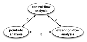
Figure 1: Relationship among exception-flow analysis, control-flow analysis and points-to analysis.

Edge B in Figure 1 denotes the relationship between exception-flow analysis and points-to analysis. Points-to analysis computes which abstract objects (with respect to allocation sites, calling contexts, etc.) a program variable or register can point to. Points-to analysis affects exception-flow analysis, because the type of the exception at a throw site determines which catch block will be executed. That is to say, exception-flow analysis requires precise points-to analysis. Similarly, exceptional flows affect points-to analysis, since the path taken by the exceptional flow can enable or disable object assignments and bindings.

The mutually recursive relationship of CFA and points-to analysis, denoted by edge C, is obvious: abstract objects (points-to analysis) determine which methods can be resolved in dynamic dispatch (CFA), while control-flow paths affect object assignments and bindings for points-to analysis. In fact, exception-flow analysis is an example of this relationship, which exacerbates the edge C relationship further!

I-A Existing approaches

Existing compilers or analysis frameworks provide a conservative model for exception handling. One approach assigns all exceptions thrown in a program to a single global variable. This variable is then read at an exception catch site. This approach is imprecise since it has no knowledge of which exception propagates to a catch site [13, 20].

The second approach analyzes exceptional control flow only intra-procedurally, computing only local catch clauses for a try block, with no dynamic propagation of exceptions inter-procedurally.

The third approach is co-analysis using both control-flow analysis and points-to analysis (a.k.a. on-the-fly control-flow construction) to handle exceptions, which yields reasonable precision, compared to the aforementioned two approaches, as documented in a past precision study [6]. Unfortunately, even for the best co-analysis, where boosting context-sensitivity improves the analysis of exceptions, it does not improve as much as it does for points-to analysis. It is too easy for exceptions to cross context boundaries and merge. For the previous simple example, we could increase to 1-call-site sensitivity. However, context-sensitivity costs more and is easily confused when calls are wrapped, as in:

 try {

    callsMaybeThrow();  // Call 1

 } catch (Exception e) {  // Handler 1

    System.err.println("Got an exception");

 }

 callsMaybeThrow();  // Call 2

 // ...

 void callsMaybeThrow() {

   maybeThrow();

 }

Similarly, values can easily merge with finitized object-sensitivity in points-to analysis. For example, if object-sensitivity uses $k$ levels of object allocation sites (or a mix with receiver objects) to distinguish contexts, objects are merged when the level exceeds $k$. Even worse, the limited $k$-sensitivity does not distinguish live heap objects from dead (garbage) heap objects, the existence of which harms both the precision and performance of the analysis. More detailed related work is described in Section IX.

I-B Our approach

Due to the intrinsic relationships illustrated in Figure 1, we propose a hybrid joint analysis of pushdown exception-flow analysis with abstract garbage collection enhanced with liveness analysis. Specifically, a pushdown system derived from the concrete semantics of a core calculus for an object-oriented language extended with exceptions is used to tackle exceptional control-flow matching between catches and throws, in addition to call and return matches. Abstract garbage collection is adapted to an object-oriented program setting, and it is enhanced with liveness analysis to tackle the points-to aspect of exception-flow analysis. We evaluate an implementation for Dalvik bytecode of the joint analysis technique on a standard set of Java benchmarks. The results show that the pruned, pushdown exception-flow analysis yields higher precision than traditional exception-flow analysis by up to 11 times within a reasonable amount of analysis time.

I-C Organization

The rest of the paper is organized as follows: Section II presents the core calculus of an object-oriented language extended with exceptions. Section III formulates the concrete semantics for the language with the intent of refactoring and abstracting it into a static analyzer. Section IV derives the abstract semantics from the concrete semantics by reformulating the structure of continuations into a list of frames and forms an implicit pushdown system. Section V-A introduces the adaptation of abstract garbage collection in object-oriented languages. Section V-B enhances the adapted abstract garbage collection with liveness analysis for better precision. The reachability algorithm is described in Section VI. Section VII describes the details of our implementation. The evaluation and benchmarks are reported in Section VIII. Section IX reports related work, and Section X concludes.

II A Featherweight Java with Exceptions

For presentation purpose, we start with a variant of Featherweight Java [14] in “A-Normal” form [11] with exceptions. A-Normal Featherweight Java (ANFJ) is identical to ordinary Featherweight Java, except that arguments to a function call must be atomically evaluable, as they are in A-Normal Form $\lambda$-calculus. For example, the body return f.foo(b.bar()); becomes the sequence of statements

B b1 = b.bar();

F f1 = f.foo(b1);

return f1;

This does not change the expressive power of the language or the nature of the analysis to come, but it does simplify the semantics while preserving the essence of the language.

The following grammar describes A-Normal Featherweight Java extended with exceptions; like regular Java, ANFJ has statement forms:

$$\mathsf{Class} \mathrel{::=}\mathtt{class}\;C\;\mathtt{extends}\;C^{\prime}\;\mbox{\tt\{}\overrightarrow{C^{\prime\prime}\;f\;\mbox{\tt;}}\;K\;\overrightarrow{M}\mbox{\tt\}}$$

$$K\in\mathsf{Konst} \mathrel{::=}C\;\mbox{\tt(}\overrightarrow{C\;f\;}\mbox{\tt)}\mbox{\tt\{}\mathtt{super}\mbox{\tt(}\overrightarrow{f^{\prime}}\mbox{\tt)}\;\mbox{\tt;}\;\overrightarrow{\mathtt{this}\mbox{\tt.}f^{\prime\prime}\mathrel{=}f^{\prime\prime\prime}\mbox{\tt;}}\mbox{\tt\}}$$

$$M\in\mathsf{Method} \mathrel{::=}C\;m\;\mbox{\tt(}\overrightarrow{C\;v\;}\mbox{\tt)}\;\mbox{\tt\{}\;\overrightarrow{C\;v\;\mbox{\tt;}}\;\vec{s}\;\mbox{\tt\}}$$

$$s\in\mathsf{Stmt} \mathrel{::=}v=e\;\mbox{\tt;}^{\ell}$$

$$\;\;\mathrel{|}\;\;\texttt{return}\;v\;\mbox{\tt;}^{\ell}$$

$$\;\;\mathrel{|}\;\;\texttt{try}\;\{\vec{s}\}\;\texttt{catch}\;\mbox{\tt(}C\;\;v\mbox{\tt)}\;\{\vec{s}^{\prime}\}^{\ell}$$

$$\;\;\mathrel{|}\;\;\texttt{throw}\;v\;\mbox{\tt;}^{\ell}$$

$$e\in\mathsf{Exp} \mathrel{::=}v\mathrel{|}v\mbox{\tt.}f\mathrel{|}v\mbox{\tt.}m\mbox{\tt(}\overrightarrow{v}\mbox{\tt)}\mathrel{|}\mathtt{new}\;C\;\mbox{\tt(}\overrightarrow{v}\mbox{\tt)}\mathrel{|}\mbox{\tt(}C\mbox{\tt)}v$$

$$f\in\mathsf{FieldName} =\mathsf{Var}$$

$$C\in\mathsf{ClassName}$$ is a set of class names

$$m\in\mathsf{MethodCall}$$ is a set of method invocation sites

$$\ell\in\mathsf{Lab}$$ is a set of labels

$$v\in\mathsf{Var}$$ is a set of variables

The set $\mathsf{Var}$ contains both variable and field names. Every statement has a label. The function $\mathit{succ}:\mathsf{Lab}\rightharpoonup\mathsf{Stmt}$ yields the (semantically) subsequent statement for a statement’s label.

III Machine semantics for Featherweight Java

$$\varsigma\in\Sigma =\mathsf{Stmt}\times\mathit{FramePointer}\times\mathit{Store}\times\mathit{Kont}\times\mathit{Time}$$

$$\sigma\in\mathit{Store} =\mathit{Addr}\rightharpoonup\mathit{D}$$

$$d\in D =\mathit{Val}$$

$$\mathit{val}\in\mathit{Val} =\mathit{Obj}$$

$$o\in\mathit{Obj} =\mathsf{ClassName}\times\mathit{ObjectPointer}$$

$$\kappa\in\mathit{Kont} \mathrel{::=}\mathbf{fun}(v,s,\mathit{fp},\kappa)$$

$$\;\;\mathrel{|}\;\;\mathbf{handle}(C,v,\vec{s},\mathit{fp},\kappa)$$

$$\;\;\mathrel{|}\;\;\mathbf{halt}$$

$$\mathit{fp}\in ~{}\mathit{FramePointer}\text{ is a set of frame pointers }$$

$$\mathit{op}\in ~{}\mathit{ObjectPointer}\text{ is a set of object pointers}$$

$$\mathit{ptr}\in\mathit{Ptr} =\mathit{FramePointer}+\mathit{ObjectPointer}$$

$$a\in\mathit{Addr} =(\mathsf{Var}+\mathsf{Method})\times\mathit{Ptr}$$

$$t\in\mathit{Time}$$ is a set of time-stamps.

Figure 2: Concrete state-space for A-Normal Featherweight Java.

$${\mathcal{C}} :\mathsf{ClassName}\to(\mathsf{FieldName}^{*}\times\mathit{Ructor})$$

$${\mathcal{K}} \in\mathit{Ructor}=\overbrace{\mathit{Addr}^{*}}^{\text{fields}}\times\overbrace{D^{*}}^{\text{arguments}}\to(\overbrace{\mathit{Store}}^{\text{field values}}\times\overbrace{\mathit{ObjectPointer}}^{\text{record}})$$

$${\mathcal{M}} :\mathit{D}\times\mathsf{MethodCall}\rightharpoonup\mathsf{Method}$$

Figure 3: Helper functions for the concrete semantics.

In preparation for synthesizing an abstract interpreter, we first construct a small-step abstract machine-based semantics for Featherweight Java. Figure 2 contains the concrete state-space for the small-step Featherweight Java machine. Each machine state has five components: a statement, a frame pointer, a store, a continuation and a timestamp. The encoding of objects abstracts over a low-level implementation: an object is a class plus a base pointer, and field addresses are “offsets” from this base pointer. Given an object $(C,\mathit{op})$, the address of field $f$ would be $(f,\mathit{op})$. In the semantics, object allocation creates a single new base object pointer $\mathit{op}^{\prime}$.

The concrete semantics use the helper functions described in Figure 3. The constructor-lookup function ${\mathcal{C}}$ yields the field names and the constructor associated with a class name. A constructor ${\mathcal{K}}$ takes a newly allocated address to use for fields and a vector of arguments; it returns the change to the store plus the record component of the object that results from running the constructor. The method-lookup function ${\mathcal{M}}$ takes a method invocation point and an object to determine which method is actually being called at that point. The concrete semantics are encoded as a small-step transition relation, $(\mathrel{\Rightarrow})\subseteq\Sigma\times\Sigma$. Each statement and expression type has a transition rule below.

Variable reference

Variable reference computes the address relative to the current frame pointer and retrieves the result from the store:

$$([\![{v=v^{\prime}\mbox{\tt;}^{\ell}}]\!],\mathit{fp},\sigma,\kappa,t)\mathrel{\Rightarrow}(\mathit{succ}(\ell),\mathit{fp},\sigma^{\prime},\kappa,t^{\prime}),$$

$$\text{ where }t^{\prime}={{tick}}(\ell,t),~{}\sigma^{\prime}=\sigma[(v,\mathit{fp})\mapsto\sigma(v^{\prime},\mathit{fp})]\text{.}$$

Return to call

Returning from a function checks if the top-most frame pointer is a function continuation (as apposed to an exception-handler continuation). If it is, then the machine binds the result and restores the context of the continuation; if not, then the machine skips to the next continuation. If $\kappa=\mathbf{fun}(v^{\prime},s,\mathit{fp}^{\prime},\kappa^{\prime})$:

$$([\![{\texttt{return}\;v\;\mbox{\tt;}^{\ell}}]\!],\mathit{fp},\sigma,\kappa,t)\mathrel{\Rightarrow}(s,\mathit{fp}^{\prime},\sigma^{\prime},\kappa^{\prime},t^{\prime})\text{, where }$$

$$t^{\prime}={{tick}}(\ell,t),~{}\sigma^{\prime}=\sigma[(v^{\prime},\mathit{fp})\mapsto d],~{}d=\sigma(v,\mathit{fp})\text{.}$$

Return over handler

If the topmost continuation is a handler, then the machine pops the handler off the stack. So, if $\kappa=\mathbf{handle}(C,v,\vec{s},\mathit{fp}^{\prime},\kappa^{\prime})$:

$$([\![{\texttt{return}\;v\;\mbox{\tt;}^{\ell}}]\!],\mathit{fp},\sigma,\kappa,t)\mathrel{\Rightarrow}([\![{\texttt{return}\;v\;\mbox{\tt;}^{\ell}}]\!],\mathit{fp},\sigma,\kappa^{\prime},t^{\prime})$$

$$\text{ where }t^{\prime}={{tick}}(\ell,t)\text{.}$$

Field reference

Field reference is similar to variable reference, except that it must find the base object pointer with which to compute the appropriate offset:

$$([\![{v=v^{\prime}\mbox{\tt.}f\;\mbox{\tt;}^{\ell}}]\!],\mathit{fp},\sigma,\kappa,t)\mathrel{\Rightarrow}(\mathit{succ}(\ell),\mathit{fp},\sigma^{\prime},\kappa,t^{\prime}),$$

$$\text{ where }t^{\prime}={{tick}}(\ell,t),$$

$$(C,{\mathit{op}}^{\prime})=\sigma(v^{\prime},\mathit{fp}),~{}\sigma^{\prime}=\sigma[(v,\mathit{fp})\mapsto\sigma(f,{\mathit{op}}^{\prime})]\text{.}$$

Method invocation

Method invocation is a multi-step process: it looks up the object, determines the class of the object and then identifies the appropriate method. When transitioning to the body of the resolved method, a new function continuation is instantiated, which records the caller’s execution context. Finally, the store is updated with the bindings of formal parameters to evaluated values of passed arguments.

$$\begin{split}&([\![{v=v_{0}\mbox{\tt.}m\mbox{\tt(}\overrightarrow{v^{\prime}}\mbox{\tt)}\mbox{\tt;}^{\ell}}]\!],\mathit{fp},\sigma,\kappa,t)\mathrel{\Rightarrow}(s_{0},\mathit{fp}^{\prime},\sigma^{\prime},\kappa^{\prime},t^{\prime}),\end{split}$$

$$\text{ where }M=[\![{C\;m\;\mbox{\tt(}\overrightarrow{C\;v^{\prime\prime}\;}\mbox{\tt)}\;\mbox{\tt\{}\overrightarrow{C^{\prime}\;v^{\prime\prime\prime}\;\mbox{\tt;}}\;\vec{s}\mbox{\tt\}}}]\!]={\mathcal{M}}(d_{0},m)$$

$$d_{0}=\sigma(v_{0},\mathit{fp}),d_{i}=\sigma(v^{\prime}_{i},\mathit{fp}),t^{\prime}={{tick}}(\ell,t),\mathit{fp}^{\prime}=\mathit{alloc}(\ell,t^{\prime}),$$

$$\kappa^{\prime}=\mathbf{fun}(v,\mathit{succ}(\ell),\mathit{fp},\kappa),a^{\prime}_{i}=(v_{i}^{\prime\prime},\mathit{fp}^{\prime}),\sigma^{\prime}=\sigma[a^{\prime}_{i}\mapsto d_{i}]\text{.}$$

Object allocation

Object allocation creates a new base object pointer; it also invokes the constructor helper to initialize the object( The $(+)$ operation represents right-biased functional union in that wherever vector $\vec{x}$ is in scope, its components are implicitly in scope: $\vec{x}=\langle x_{0},\ldots,x_{\mathit{length(\vec{x})}}\rangle$):

$$\begin{split}&([\![{v={\tt new}\;C\;\mbox{\tt(}\overrightarrow{v^{\prime}}\mbox{\tt)}\mbox{\tt;}^{\ell}}]\!],\mathit{fp},\sigma,\kappa,t)\mathrel{\Rightarrow}(\mathit{succ}(\ell),\mathit{fp},\sigma^{\prime},\kappa,t^{\prime})\text{,}\\ \end{split}$$

$$\text{ where }t^{\prime}={{tick}}(\ell,t),~{}~{}d_{i}=\sigma(v_{i}^{\prime},\mathit{fp}),~{}~{}(\vec{f},{\mathcal{K}})={\mathcal{C}}(C),~{}~{}$$

$$\mathit{fp}^{\prime}=\mathit{alloc}(\ell,t^{\prime}),~{}~{}a_{i}=(f_{i},\mathit{fp}^{\prime})(\Delta\sigma,{\mathit{op}}^{\prime})={\mathcal{K}}(\vec{a},\vec{d}),~{}~{}$$

$$d^{\prime}=(C,{\mathit{op}}^{\prime}),~{}~{}\sigma^{\prime}=\sigma+\Delta\sigma+[(v,\mathit{fp})\mapsto d^{\prime}]\text{.}$$

Casting

A cast references a variable, replacing the class of the object:

$$([\![{v=\mbox{\tt(}C^{\prime}\mbox{\tt)}\;v^{\prime}}]\!],\mathit{fp},\sigma,\kappa,t)\mathrel{\Rightarrow}(\mathit{succ}(\ell),\mathit{fp},\sigma^{\prime},\kappa,t^{\prime}),$$

$$\text{ where }t^{\prime}={{tick}}(\ell,t),~{}~{}\sigma^{\prime}=\sigma[(v,\mathit{fp})\mapsto\sigma(v^{\prime},\mathit{fp})]\text{.}$$

Try

A try statement creates a new handler continuation and then proceeds to the body of the try statement.

$$([\![{\texttt{try}\;\{\vec{s}\}\;\texttt{catch}\;\mbox{\tt(}C\;\;v\mbox{\tt)}\;\{\vec{s}^{\prime}\}^{\ell}}]\!],\mathit{fp},\sigma,\kappa,t)$$

$$\mathrel{\Rightarrow}(\mathit{succ}(\ell),\mathit{fp},\sigma,\kappa^{\prime},t^{\prime})$$

$$\text{ where }t^{\prime}={{tick}}(\ell,t),~{}~{}\kappa^{\prime}=\mathbf{handle}(C,v^{\prime},s^{\prime}_{1},\mathit{fp},\kappa)\text{.}$$

Throw to matching handler

When the machine encounters a throw statement, it must check if the topmost continuation is both a handler and a matching handler; if so, then it returns to the context within the continuation: If $\kappa=\mathbf{handle}(C^{\prime},v^{\prime},s,\mathit{fp}^{\prime\prime},\kappa^{\prime})$ and $\sigma(v,\mathit{fp})=(C,{\mathit{op}}^{\prime})$ and $C$ is a $C^{\prime}$:

$$([\![{\texttt{throw}\;v\;\mbox{\tt;}^{\ell}}]\!],\mathit{fp},\sigma,\kappa,t)\mathrel{\Rightarrow}(s,\mathit{fp}^{\prime\prime},\sigma^{\prime},\kappa^{\prime},t^{\prime})$$

$$\text{where~{}~{} }t^{\prime}={{tick}}(\ell,t),~{}~{}\sigma^{\prime}=\sigma[(v^{\prime},\mathit{fp}^{\prime\prime})\mapsto(C,{\mathit{op}}^{\prime})]\text{.}$$

Throw past non-matching handler

When throwing, if the topmost handler is not a match, the machine looks deeper in the stack for a matching handler. If $\kappa=\mathbf{handle}(C^{\prime},v^{\prime},s,\mathit{fp}^{\prime\prime},\kappa^{\prime})$ and $\sigma(v,\mathit{fp})=(C,{\mathit{op}}^{\prime})$ but $C$ is not a $C^{\prime}$:

$$([\![{\texttt{throw}\;v\;\mbox{\tt;}^{\ell}}]\!],\mathit{fp},\sigma,\kappa,t)\mathrel{\Rightarrow}([\![{\texttt{throw}\;v\;\mbox{\tt;}^{\ell}}]\!],\mathit{fp},\sigma,\kappa^{\prime},t^{\prime})$$

$$\text{where ~{}~{} }t^{\prime}={{tick}}(\ell,t)\text{.}$$

Throw past return point

If throwing an exception and the topmost handler is a function return point, then it jumps over this continuation. If $\kappa=\mathbf{fun}(v^{\prime},s,\mathit{fp}^{\prime},\kappa^{\prime})$:

$$([\![{\texttt{throw}\;v\;\mbox{\tt;}^{\ell}}]\!],\mathit{fp},\sigma,\kappa,t)\mathrel{\Rightarrow}([\![{\texttt{throw}\;v\;\mbox{\tt;}^{\ell}}]\!],\mathit{fp},\sigma,\kappa^{\prime},t^{\prime})$$

$$\text{where ~{}~{} }t^{\prime}={{tick}}(\ell,t)\text{.}$$

Popping handlers

When control passes out of a try block, the topmost handler must be popped from the stack. To handle this, the “successor” of the last statement in a try block is actually a special pophandler statement, and the “successor” of that statement is the statement directly following the try block.

$$([\![{\texttt{pophandler}\;\mbox{\tt;}^{\ell}}]\!],\mathit{fp},\sigma,\kappa,t)\mathrel{\Rightarrow}(\mathit{succ}(\ell),\mathit{fp},\sigma,\kappa^{\prime},t^{\prime})$$

$$\text{ where ~{}~{} }t^{\prime}={{tick}}(\ell,t),~{}~{}\kappa=\mathbf{handle}(\ldots,\kappa^{\prime})\text{.}$$

IV A pushdown semantics of exceptions

$${\hat{\varsigma}}\in{\hat{\Sigma}}=\mathsf{Stmt} \times\widehat{\mathit{FramePointer}}\times\widehat{\mathit{Store}}\times\widehat{\mathit{Kont}}\times\widehat{\mathit{Time}}$$

$${\hat{\sigma}}\in\widehat{\mathit{Store}} =\widehat{\mathit{Addr}}\rightharpoonup\widehat{\mathit{D}}$$

$${\hat{d}}\in\hat{D} ={\mathcal{P}\left(\widehat{\mathit{Val}}\right)}$$

$${\widehat{\mathit{val}}}\in\widehat{\mathit{Val}} =\widehat{\mathit{Obj}}$$

$${\hat{o}}\in\widehat{\mathit{Obj}} =\mathsf{ClassName}\times\widehat{\mathit{ObjectPointer}}$$

$${\hat{\kappa}}\in\widehat{\mathit{Kont}} =\widehat{\mathit{Frame^{*}}}$$

$$\hat{\phi}\in\widehat{\mathit{Frame}} =\widehat{\mathit{CallFrame}}+\widehat{\mathit{HandlerFrame}}$$

$$\widehat{\chi}\in\widehat{\mathit{CallFrame}} ::=\mathbf{fun}(v,s,\hat{\mathit{fp}})$$

$$\widehat{\eta}\in\widehat{\mathit{HandlerFrame}} ::=\mathbf{handle}(C,v,\vec{s},\hat{\mathit{fp}})$$

$$\hat{\mathit{fp}}\in\widehat{\mathit{FramePointer}}$$ is a set of frame pointers

$$\widehat{\mathit{op}}\in\widehat{\mathit{ObjectPointer}}$$ is a set of object pointers

$$\widehat{\mathit{ptr}}\in\widehat{\mathit{Ptr}} =\widehat{\mathit{FramePointer}}+\widehat{\mathit{ObjectPointer}}$$

$${\hat{a}}\in\widehat{\mathit{Addr}} =(\mathsf{Var}+\mathsf{Method})\times\widehat{\mathit{Ptr}}$$

$${\hat{t}}\in\widehat{\mathit{Time}}$$ is a set of time-stamps.

Figure 4: Abstract state-space for pushdown analysis of A-Normal Featherweight Java.

With the concrete semantics for A-Normal Featherweight Java with exceptions in place, we are ready to derive the abstract semantics for static analysis. “Abstracting abstract machines” (AAM) has proposed a systematic approach to derive such kind of abstraction, which is equivalent to most of the conservative static analyses [32]. The idea is to make the analysis finite and terminate by finitize every component in the state, so that there is no source of infinity. However, when we apply this technique, the precision is not satisfiable in the client security analysis [21], because the over-approximation of the continuation component causes spurious control-flow and return-flows.

Therefore, in this work, we choose to abstract less than what AAM approach does: we leave the stack (represented as continuation) unbounded in height. In fact, the central idea behind this abstraction is the generalization of two kinds of frames on stack: the function frames and the exception-handler frames. In this way, we form the abstract pushdown semantics. Then, the pushdown abstract semantics will further be computed as control-state reachability in pushdown systems, which is evolved from the work of [26, 9, 10]. However, unlike them, we improve the algorithm to handle new behaviors introduced by exceptions. The algorithm is detailed in Section VI. The rest of the section focuses how we formulate the pushdown semantics.

Abstract semantics are defined on an abstract state-space. To formulate the pushdown abstract state-space, we first reformulate continuations as a list of frames in the concrete semantics:

$$\mathit{Kont} \cong\mathit{Frame}^{*}$$

$$\mathit{Frame} =\mathit{CallFrame}+\mathit{HandlerFrame}$$

$$\mathit{CallFrame} ::=\mathbf{fun}(v,s,\mathit{fp})$$

$$\mathit{HandlerFrame} ::=\mathbf{handle}(C,v,\vec{s},\mathit{fp})\text{.}$$

We have two kinds of frames: function frames as well as handler frames. As with continuations, they may grow without bound (The enhanced reachability algorithm handles this in Section VI).

Figure 4 contains the abstract state-space for the pushdown version of the small-step Featherweight Java machine. At this point, we can extract the high-level structure of the pushdown system from the state-space. A configuration in a pushdown system is a control state (from a finite set) paired with a stack (with a finite number of frames that are defined in Figure 4). This can be observed as follows:

$${\hat{\Sigma}} =\mathsf{Stmt}\times\widehat{\mathit{FramePointer}}\times\widehat{\mathit{Store}}\times\widehat{\mathit{Kont}}\times\widehat{\mathit{Time}}$$

$$\cong\mathsf{Stmt}\times\widehat{\mathit{FramePointer}}\times\widehat{\mathit{Store}}\times\widehat{\mathit{Time}}\times\widehat{\mathit{Kont}}$$

$$=\left(\mathsf{Stmt}\times\widehat{\mathit{FramePointer}}\times\widehat{\mathit{Store}}\times\widehat{\mathit{Time}}\right)\times\widehat{\mathit{Kont}}$$

$$=\underbrace{\left(\mathsf{Stmt}\times\widehat{\mathit{FramePointer}}\times\widehat{\mathit{Store}}\times\widehat{\mathit{Time}}\right)}_{\text{control states}}\times\underbrace{\widehat{\mathit{Frame}}^{*}}_{\text{stack}}$$

Now let us show the detailed abstract transition relations. Thanks to the way we do the abstraction so far (That is, structural abstraction of concrete states except for the stack component), the abstract transition relations resemble a lot as their concrete counterparts. The biggest difference in abstract semantics is that it does weak updates using the operator $\sqcup$. For example, for variable reference (weak updates are underlined.):

$$([\![{v=v^{\prime}\mbox{\tt;}^{\ell}}]\!],\hat{\mathit{fp}},{\hat{\sigma}},{\hat{\kappa}},{\hat{t}})\leadsto(\mathit{succ}(\ell),\hat{\mathit{fp}},{\hat{\sigma}}^{\prime},{\hat{\kappa}},{\hat{t}}^{\prime})\text{,}$$

$$\text{ where }{\hat{t}}^{\prime}={\widehat{tick}}(\ell,{\hat{t}})\text{ and }\underline{{\hat{\sigma}}^{\prime}={\hat{\sigma}}\sqcup[(v,\hat{\mathit{fp}})\mapsto\sigma(v^{\prime},\hat{\mathit{fp}})]}$$

The other difference is, whenever evaluating expressions, the results are abstract entities that represents one or more concrete entities. For example, field reference:

$$([\![{v=v^{\prime}\mbox{\tt.}f\;\mbox{\tt;}^{\ell}}]\!],\hat{\mathit{fp}},{\hat{\sigma}},{\hat{\kappa}},{\hat{t}})\leadsto(\mathit{succ}(\ell),\hat{\mathit{fp}},{\hat{\sigma}}^{\prime},{\hat{\kappa}},{\hat{t}}^{\prime})$$

$$\text{ where }{\hat{t}}^{\prime}={\widehat{tick}}(\ell,{\hat{t}}),\underline{(C,\widehat{\mathit{op}}^{\prime})\in{\hat{\sigma}}(v^{\prime},\hat{\mathit{fp}})},{\hat{\sigma}}^{\prime}={\hat{\sigma}}\sqcup[(v,\hat{\mathit{fp}})\mapsto{\hat{\sigma}}(f,\widehat{\mathit{op}}^{\prime})]$$

The underlined operation shows that there could be more than one abstract objects are evaluated. The two differences apply to all the other rules. To save space, we demonstrate the abstract rules that involve exceptions. Fig 5 shows how we handle the exception-flow and its mix with normal control-flow. The idea is the “multi-pop” behavior introduced when a function call returns or an exception throws (as the concrete semantics). The effect of this approach substantially simplifies the control-reachability algorithm during summarization, as we shall show in Section VI.

[Try]: $$\displaystyle([\![{\texttt{try}\;\{\vec{s}\}\;\texttt{catch}\;\mbox{\tt(}C\;\;v\mbox{\tt)}\;\{\vec{s}^{\prime}\}^{\ell}}]\!],\hat{\mathit{fp}},{\hat{\sigma}},{\hat{\kappa}},{\hat{t}})$$ $$\displaystyle\leadsto(\mathit{succ}(\ell),\hat{\mathit{fp}},{\hat{\sigma}},{\hat{\kappa}}^{\prime},{\hat{t}}^{\prime}),$$ $$\displaystyle\text{ where }{\hat{t}}^{\prime}={\widehat{tick}}(\ell,{\hat{t}})\text{ and }{\hat{\kappa}}^{\prime}=\mathbf{handle}(C,v^{\prime},s^{\prime}_{1},\hat{\mathit{fp}})::{\hat{\kappa}}\text{.}$$ [Throw to matching handler]: $$\displaystyle([\![{\texttt{throw}\;v\;\mbox{\tt;}^{\ell}}]\!],\hat{\mathit{fp}},{\hat{\sigma}},{\hat{\kappa}},{\hat{t}})\leadsto(s,\hat{\mathit{fp}}^{\prime\prime},{\hat{\sigma}}^{\prime},{\hat{\kappa}}^{\prime},{\hat{t}}^{\prime})\text{,}$$ $$\displaystyle\text{ where }{\hat{t}}^{\prime}={\widehat{tick}}(\ell,{\hat{t}}),{\hat{\sigma}}^{\prime}={\hat{\sigma}}\sqcup[(v^{\prime},\hat{\mathit{fp}}^{\prime\prime})\mapsto(C,\widehat{\mathit{op}}^{\prime})],$$ $$\displaystyle{\hat{\kappa}}=\mathbf{handle}(C^{\prime},v^{\prime},s,\hat{\mathit{fp}}^{\prime\prime})::{\hat{\kappa}}^{\prime},(C,\widehat{\mathit{op}}^{\prime})\in{\hat{\sigma}}(v,\hat{\mathit{fp}})\text{,}C\text{ is a }C^{\prime}\text{.}$$ [Throw past non-matching handler]: $$\displaystyle([\![{\texttt{throw}\;v\;\mbox{\tt;}^{\ell}}]\!],\hat{\mathit{fp}},{\hat{\sigma}},{\hat{\kappa}},{\hat{t}})\leadsto([\![{\texttt{throw}\;v\;\mbox{\tt;}^{\ell}}]\!],\hat{\mathit{fp}},{\hat{\sigma}},{\hat{\kappa}}^{\prime},{\hat{t}}^{\prime})\text{,}$$ $$\displaystyle\text{ where }{\hat{t}}^{\prime}={\widehat{tick}}(\ell,{\hat{t}}),{\hat{\kappa}}=\mathbf{handle}(C^{\prime},v^{\prime},s,\hat{\mathit{fp}}^{\prime\prime})::{\hat{\kappa}}^{\prime},$$ $$\displaystyle(C,\widehat{\mathit{op}}^{\prime})\in{\hat{\sigma}}(v,\hat{\mathit{fp}})\text{ and }C\text{ is not a }C^{\prime}\text{.}$$ [Throw past return point]: $$\displaystyle([\![{\texttt{throw}\;v\;\mbox{\tt;}^{\ell}}]\!],\hat{\mathit{fp}},{\hat{\sigma}},{\hat{\kappa}},{\hat{t}})\leadsto([\![{\texttt{throw}\;v\;\mbox{\tt;}^{\ell}}]\!],\hat{\mathit{fp}},{\hat{\sigma}},{\hat{\kappa}}^{\prime},{\hat{t}}^{\prime})\text{,}$$ $$\displaystyle\text{ where }{\hat{t}}^{\prime}={\widehat{tick}}(\ell,{\hat{t}}),\text{ and }{\hat{\kappa}}=\mathsf{fun}(v^{\prime},s,\hat{\mathit{fp}}^{\prime})\text{::}{\hat{\kappa}}^{\prime}\text{.}$$ [Return over handler]: $$\displaystyle([\![{\texttt{return}\;v\;\mbox{\tt;}^{\ell}}]\!],\hat{\mathit{fp}},{\hat{\sigma}},{\hat{\kappa}},{\hat{t}})\leadsto([\![{\texttt{return}\;v\;\mbox{\tt;}^{\ell}}]\!],\hat{\mathit{fp}},{\hat{\sigma}},{\hat{\kappa}}^{\prime},{\hat{t}}^{\prime}),$$ $$\displaystyle\text{ where }{\hat{t}}^{\prime}={\widehat{tick}}(\ell,{\hat{t}})\text{ and }{\hat{\kappa}}=\text{handle}(C,v,\vec{s},\hat{\mathit{fp}}^{\prime})::{\hat{\kappa}}^{\prime}\text{.}$$ [Popping handlers]: $$\displaystyle([\![{\texttt{pophandler}\;\mbox{\tt;}^{\ell}}]\!],\hat{\mathit{fp}},{\hat{\sigma}},{\hat{\kappa}},{\hat{t}})\leadsto(\mathit{succ}(\ell),\hat{\mathit{fp}},{\hat{\sigma}},{\hat{\kappa}}^{\prime},{\hat{t}}^{\prime}),$$ $$\displaystyle\text{ where }{\hat{t}}^{\prime}={\widehat{tick}}(\ell,{\hat{t}})\text{ and }{\hat{\kappa}}=\mathbf{handle}(\ldots)::{\hat{\kappa}}^{\prime}\text{.}$$

Figure 5: Abstract transition relations (exception)

V Enhanced abstract garbage collection

The previous section formulates a pushdown system to handle complicated control-flows (both normal and exceptional). This section describes how we prune the analysis for exceptions from the angle of points-to analysis with enhanced garbage collection generalized for object-oriented programs.

V-A Abstract garbage collection in an object-oriented setting

The idea of abstract garbage collection was first proposed in the work of Might and Shivers [24] for higher-order programs. As an analog to the concrete garbage collection, abstract garbage collection reallocates unreachable abstract resources. Order-of-magnitude improvements in precision have been reported, even as it drops run-times by cutting away false positives. It is natural to think that this technique can benefit exception-flow analysis for object-oriented languages. In fact, in an object-oriented setting, abstract garbage collection can free the analysis from the context-sensitivity and object-sensitivity limitation, since the “garbage” discarded is ignorant of any form of sensitivity! For example, in the following simple code snippet,

  A a1 = idA(new A());

  A a2 = idA(new A()):

  B b1 = idB(a1.makeB());

  B b2 = idB(a2.makeB());

idA and idB are identity functions. Traditionally, with one level of object-sensitivity and one level of context sensitivity, we are able to distinguish the arguments passed in all of the four lines. However, it is easy to exceed the $k$-sensitivity (call site, allocation sites, receiver objects, etc.) in modern software constructs. Abstract garbage collection can play a role in the way that it discards conservative values and enables fresh bindings for reused variables (formal parameters). This does not need knowledge about any sensitivity! Thus, it can avoid “merging” of abstract object values (and so indirectly eliminate potentially spurious function calls). For exceptions specifically, abstract garbage collection can help avoid conflating exception objects at various throw sites.

To gain the promised analysis precision and performance, we must conduct a careful and subtle redesign of the abstract garbage collection machinery for object-oriented languages. Specifically, we need to make it work with the abstract semantics defined in Section IV. In addition, the reachability algorithm should also be able to work with abstract garbage collection. Fortunately, the challenge of how to adapt abstract garbage collection into pushdown systems has been resolved in the work of Earl et al. [10]. Here we focus on the enhanced machinery for object-oriented languages.

First, we describe how we adapt abstract garbage collection to analyze object-oriented languages. Abstract garbage collection discards unreachable elements from the store, it modifies the transition relation to conduct a “stop-and-copy” garbage collection before each transition. To do so, we define a garbage collection function ${\hat{G}}:{\hat{\Sigma}}\to{\hat{\Sigma}}$ on configurations:

$${\hat{G}}(\overbrace{\vec{s},\hat{\mathit{fp}},{\hat{\sigma}},{\hat{\kappa}},{\hat{t}}}^{{\hat{\varsigma}}}) =(\vec{s},\hat{\mathit{fp}},{\hat{\sigma}}|\mathit{Reachable}({\hat{\varsigma}}),{\hat{\kappa}})\text{,}$$

where the pipe operation $f|S$ yields the function $f$, but with inputs not in the set $S$ mapped to bottom—the empty set. The reachability function $\mathit{Reachable}:{\hat{\Sigma}}\to{\mathcal{P}(\widehat{\mathit{Addr}})}$ first computes the root set and then the transitive closure of an address-to-address adjacency relation:

$$\mathit{Reachable}(\overbrace{\vec{s},\hat{\mathit{fp}},{\hat{\sigma}},{\hat{\kappa}},{\hat{t}}}^{\hat{\varsigma}}) =\left\{{\hat{a}}:{\hat{a}}_{0}\in\mathit{Root}({\hat{\varsigma}})\text{ and }{\hat{a}}_{0}\mathrel{\operatorname*{\rightarrowtriangle}_{\hat{\sigma}}^{*}}{\hat{a}}\right\}\text{,}$$

where the function $\mathit{Root}:{\hat{\Sigma}}\to{\mathcal{P}(\widehat{\mathit{Addr}})}$ finds the root addresses:

$$\mathit{Root}(\vec{s},\hat{\mathit{fp}},{\hat{\sigma}},{\hat{\kappa}},{\hat{t}})=\{(v,\hat{\mathit{fp}}):(v,\hat{\mathit{fp}})\in\mathit{dom}({\hat{\sigma}})\}\cup\mathit{StackRoot}({\hat{\kappa}})$$

The $\mathit{StackRoot}:\widehat{\mathit{Kont}}\to{\mathcal{P}(\widehat{\mathit{Addr}})}$ function finds roots on the stack. However, only $\widehat{\mathit{CallFrame}}$ has the component to construct addresses, so we define a helper function $\hat{\mathcal{F}}:\widehat{\mathit{Kont}}\to\widehat{\mathit{CallFrame}}^{*}$ to extract only $\widehat{\mathit{CallFrame}}$ out from the stack and skip over all the handle frames. Now $\mathit{StackRoot}$ is defined as

$$\mathit{StackRoot}({\hat{\kappa}})=\{(v,\hat{\mathit{fp}}_{i}):(v,\hat{\mathit{fp}}_{i})\in\mathit{dom}({\hat{\sigma}})~{}\text{and}~{}\hat{\mathit{fp}}_{i}\in\hat{\mathcal{F}}({\hat{\kappa}})\}\text{,}$$

and the relation:$(\operatorname*{\rightarrowtriangle})\subseteq\widehat{\mathit{Addr}}\times\widehat{\mathit{Store}}\times\widehat{\mathit{Addr}}$ connects adjacent addresses: ${\hat{a}}\mathrel{\operatorname*{\rightarrowtriangle}_{\hat{\sigma}}}{\hat{a}}^{\prime}\text{ iff there exists }(C,\widehat{\mathit{op}})\in{\hat{\sigma}}({\hat{a}})$ such that ${\hat{a}}^{\prime}\in\{(f,\widehat{\mathit{op}}):(f,\widehat{\mathit{op}})\in\mathit{dom}({\hat{\sigma}})\}$. The formulated abstract garbage collection semantics constructs the subroutine eagc that is called in Alg. 4, which is the interface to enable abstract garbage collection in the reachability algorithm.

V-B Abstract garbage collection enhanced with liveness analysis

Abstract garbage collection can avoid conflating abstract objects for reused variables or formal parameters, but it can not discover “garbage” or “dead” abstract objects in the local scope. The following example illustrates this:

bool foo(A a) {

  B b = B.read(a);

  C p = C.doSomething(b);

  return bar(C.not(p));

}

Obviously, in the function body foo, b is actually “dead” after the second line. However, näive abstract garbage collection has no knowledge of this. In fact, this is a problem for näive concrete garbage collection [1]. In the realm of static analysis, the garbage value pointed to by b can pollute the exploration of the entire state space.

In addition, in the register-based byte code that our implementation analyzes, there are obvious cases where the same register is reassigned multiple times at different sites within a method. The direct adaptation of abstract garbage collection to an object-oriented setting in Section V-A cannot collect these registers between uses. In other words, for object-oriented programs, we also want to collect “dead” registers, even though they are reachable under description in Section V-A. This can be easily achieve by using liveness analysis. Of course, we could also solve it by transforming the byte code into Static Single Assignment (SSA) form. However, as mentioned above, liveness analysis has additional benefits, so we chose to enhance the abstract garbage collection with live variable analysis (LVA).

LVA computes the set of variables that are alive at each statement within a method. The garbage collector can then more precisely collect each frame.

Since LVA is well-defined in the literature [2], we skip the formalization here, but the $\mathit{Root}$ is now modified to collect only live variables of the current statement $\mathit{Lives}(s_{0})$:

$$\mathit{Root}(\vec{s},\hat{\mathit{fp}},{\hat{\sigma}},{\hat{\kappa}})=\{(v^{\prime},\hat{\mathit{fp}})\}\cup\mathit{StackRoot}({\hat{\kappa}}),$$

$$\text{ where }(v^{\prime},\hat{\mathit{fp}})\in\mathit{dom}({\hat{\sigma}})~{}\text{and}~{}v^{\prime}\in\mathit{Lives}(s_{0})\text{.}$$

The liveness property is embedded in the overall eagc subroutine in Alg. 4.

VI Extending pushdown reachability analysis for exceptions

Given the formalisms in the previous sections, it is not immediately clear how to convert these rules into a static analyzer, or more importantly, how to handle the unbounded stack without it always visiting new machine configurations. Thus, we need a way to compute a finite summary of the reachable machine configurations.

In abstract interpretation frameworks, the Dyck State Graph synthesis algorithm [9], which is a purely functional version of the Saturation algorithm [26], provides a method for computing reachable pushdown control states. We build our algorithms on the work of Earl et al. [10]. As it turns out, it is not hard to extend the summarization idea to deal with an unbounded stack with exceptions. In the following sections, we present the complete algorithm in a top-down fashion, which aims to easily turn into actual working code. The algorithm code uses previous definitions specified in Section IV.

VI-A Analysis setup

Input: $s$: a list of program statements (with an initial entry point $s_{0}$).

Output: Dyck State Graph $\mathit{DSG}:$ a triple of a set of control states a set of edges, and a initial state.

1 ${\hat{\sigma}}_{0}\longleftarrow$ empty store

2 $\mathit{fp}_{0}\longleftarrow$ initial empty stack frame pointer

3 ${\hat{t}}_{0}\longleftarrow$ empty list of contexts

4 ${\hat{q}}_{0}\longleftarrow(s_{0},\mathit{fp}_{0},{\hat{\sigma}}_{0},{\hat{t}}_{0})$

5 $\text{The initial working set }{W}_{0}\longleftarrow\{{\hat{q}}_{0}\}$

6 $\mathit{IECG}_{0}\longleftarrow(\emptyset,\emptyset,\emptyset,\emptyset,\emptyset,\emptyset)$

7 $\mathit{DSG}_{0}\longleftarrow(\{{\hat{q}}_{0}\},\emptyset,{\hat{q}}_{0})$

8 ($\mathit{DSG},\mathit{IECG},{\hat{\sigma}},{W}$)$\longleftarrow$Eval($\mathit{DSG}_{0},\mathit{IECG}_{0},{\hat{\sigma}}_{0},{W}_{0}$)

return $\mathit{DSG}$

Algorithm 1 Analyze

The analysis for a program starts from the Analyze function, as shown in Alg. 1. It accepts a program expression (an entry point to a program), and gives out a Dyck State Graph (DSG). Formally speaking, a DSG of a pushdown system is the subset of a pushdown system reachable over legal paths. (A path is legal if it never tries to pop $a$ when a frame other than $a$ is on top of the stack.) Note that the $\widehat{\mathit{Time}}$ component is designed for accommodating traditional analysis, depending on actual implementation. For example, the last $k$ call sites or object-allocation labels, or the mix of them. The analysis produces DSG from the subroutine Eval, which is the fix-point synthesis algorithm.

In Alg. 1, $\mathit{IECG}$ is a composed data structure used in the $\epsilon$ summarization algorithm. It is derived from the idea of an $\epsilon$ closure graph (ECG) in the work of Earl et al. [9], but supports efficient caching of $\epsilon$ closures along with transitive push frames on the stack. Specifically, $\mathit{IECG}$ = ($\overleftarrow{G},\overrightarrow{G},\overrightarrow{\mathit{TF}},\overrightarrow{\mathit{PSF}},\overleftarrow{\mathit{PFP}},\overleftarrow{\mathit{NEP}}$). The six components can be considered maps:

• $\epsilon$ predecessors $\overleftarrow{G}$: ${\hat{\Sigma}}\rightarrow\{{\hat{\Sigma}}\}$, maps a target node to the source node(s) of an $\epsilon$ edge(s)

• $\epsilon$ successors $\overrightarrow{G}$: ${\hat{\Sigma}}\rightarrow\{{\hat{\Sigma}}\}$, maps a source node to the target node(s) of an $\epsilon$ edge(s)

• top frames $\overrightarrow{\mathit{TF}}:{\hat{\Sigma}}\rightarrow\{\widehat{\mathit{Frame}}\}$, records the shallow pushed stack frame(s) for a state node.

• possible stack frames $\overrightarrow{\mathit{PSF}}:{\hat{\Sigma}}\rightarrow\{\widehat{\mathit{Frame}}\}$, compute all possible pushed stack frame of a state. It is used for abstract garbage collection.

• predecessors for push action $\overleftarrow{\mathit{PFP}}$: $({\hat{\Sigma}},\widehat{\mathit{Frame}})\rightarrow\{{\hat{\Sigma}}\}$, records source state node(s) for a pushed frame and the net-changed state. For example in the legal path: ${\hat{q}}_{0}\xrightarrow{g^{+}}{\hat{q}}_{1}\longrightarrow...\xrightarrow{g^{-}}{\hat{q}}_{2}$, the entry $({\hat{q}}_{1},g^{+})\longrightarrow\{{\hat{q}}_{0}\}$ is in $\overleftarrow{\mathit{PFP}}$.

• non-$\epsilon$ predecessors ($\overleftarrow{\mathit{NEP}}:$ ${\hat{\Sigma}}\rightarrow\{{\hat{\Sigma}}\}$), maps a state node to non-$\epsilon$ predecessors.

These data structures (and $\mathit{IECG}$) have the same definition in the following algorithms.

VI-A1 Fix-point algorithm of the pushdown exception framework

Alg. 2 describes the fix-point computation for the reachability algorithm. It iteratively constructs the reachable portion of the pushdown transition relation (Ln. 5-12) by inserting $\epsilon$-summary edges whenever it finds empty-stack (Ln. 13-20) (e.g., push a, push b, pop b, pop a) paths between control states.

Input: $\mathit{DSG},\mathit{IECG}(\text{definition referred to Section~{}\ref{subsec:setup}}),{\hat{\sigma}},\text{working set }{W}$

Output: $\mathit{DSG}^{\prime},\mathit{IECG}^{\prime},{\hat{\sigma}}^{\prime\prime},{W}^{\prime}$

1 $\varDelta{S},\varDelta{E},{\hat{\sigma}}^{\prime\prime},{W}^{\prime}\leftarrow\emptyset$

2 $(E,S,{\hat{q}}_{0})\leftarrow\mathit{DSG}$

3 $(\overleftarrow{G},\overrightarrow{G},\overrightarrow{\mathit{TF}},\overrightarrow{\mathit{PSF}},\_,\_)\leftarrow\mathit{IECG}$

4 $\mathit{IECG}^{\prime}\leftarrow(\emptyset,\emptyset,\emptyset,\emptyset,\emptyset,\emptyset)$

5 for $s$ $\in$ ${W}$ do

6       for $\hat{\kappa}$ $\in$ $\overrightarrow{\mathit{TF}}(s)$ do

7             for $(g,s_{1},{\hat{\sigma}}^{\prime})\in\mathit{\text{\sc{Step}}(s,\hat{\kappa},\overrightarrow{\mathit{PSF}}(s),{\hat{\sigma}})}$ do

8                   if $s\notin(\overrightarrow{G}(s)\cup S\cup\overleftarrow{G}(s))$ then

9                         insert $s_{1}$ in $\varDelta{S}$

10                         insert $\mathit{E(s,g,s_{1})}$ in $\varDelta{E}$

11                         insert $s_{1}$ in ${W}^{\prime}$

12                         ${\hat{\sigma}}^{\prime\prime}={\hat{\sigma}}^{\prime}\sqcup{\hat{\sigma}}$

13                  

14            

15       for $E$ $\in$ $\varDelta{E}$ do

16             switch E do

17                   case $(s^{\prime},\varepsilon,s^{\prime\prime})$

18                         $\mathit{IECG}^{\prime}\leftarrow$ Propagate($E$, $\mathit{IECG}$)

19                   case $(s^{\prime},g^{+},s^{\prime\prime})$

20                         $\mathit{IECG}^{\prime}\leftarrow$ ProcessPush($E,\mathit{IECG}$)

21                   case $(s^{\prime},g^{-},s^{\prime\prime})$

22                         $\mathit{IECG}^{\prime}\leftarrow$ ProcessPop($E,\mathit{IECG}$)

23                  

24            

25       $DSG^{\prime}\leftarrow(E\cup\varDelta{E},S\cup\varDelta{S})$

26      

27      if ${\hat{\sigma}}^{\prime\prime}\sqsubseteq{\hat{\sigma}}\wedge\varDelta{E}==\emptyset$ then

28             return ($\mathit{DSG^{\prime},\mathit{IECG}^{\prime},{\hat{\sigma}}^{\prime\prime},{W}^{\prime}}$)

29       else

30             Eval$(DSG^{\prime},\mathit{IECG}^{\prime},{\hat{\sigma}}^{\prime\prime},{W}^{\prime})$

31            

32      

Algorithm 2 Eval

Ln. 22-25 decides when to terminate the analysis: no new frontier edges and the new store component ${\hat{\sigma}}^{\prime\prime}$ is subsumed by the old store ${\hat{\sigma}}^{\prime}$. The second condition uses the technique presented by Shivers [29]. Otherwise, it recurs to Eval.

Input: control state ${\hat{q}}$, continuation ${\hat{\kappa}}$, a list of frames $\vec{\hat{\phi}}$

Output: a set of records (stack action $g$, ${\hat{q}}^{\prime}$, ${\hat{\sigma}}$)

1 $\mathit{result}\longleftarrow\emptyset$

2 for (g, ${\hat{q}}^{\prime}$) $\in$ StepIPDS(${\hat{q}}$, ${\hat{\kappa}}$, $\vec{\hat{\phi}}$) do

3       insert ($g$, ${\hat{q}}^{\prime}$, ${\hat{\sigma}}$) in $\mathit{result}$

return $\mathit{result}$

Algorithm 3 Step

Input: $\text{a source state }{\hat{q}},\text{continuation }{\hat{\kappa}},\text{list of frames }\vec{\hat{\phi}}$, $\mathit{Options}$: global analysis options

Output: a set of tuples ($\hat{\phi}^{\prime},{\hat{q}}^{\prime}$)

1 $\mathit{result}$ $\longleftarrow\emptyset$

2 ${\hat{q}}^{\prime}\longleftarrow{\hat{q}}$

3 if $\mathit{Options.doGC}$ then ${\hat{q}}^{\prime}\longleftarrow$ eagc(${\hat{q}},\hat{\phi}$)

4 $\mathit{confs}\longleftarrow$ next(${\hat{q}}^{\prime},\hat{\kappa}$)

5 for $({\hat{q}}^{\prime\prime},{\hat{\kappa}}^{\prime})\in\mathit{confs}$ do

6       g $\longleftarrow$ DecideStackAction(${\hat{\kappa}},{\hat{\kappa}}^{\prime}$)

7       insert (g, ${\hat{q}}^{\prime\prime}$) in $\mathit{result}$

8      

return $\mathit{result}$

Algorithm 4 StepIPDS

Now we explain Ln. 5-12 in more detail by examining the subroutines that are called. As is shown in Ln. 7, the raw new states and edges are obtained from calling Step (shown in Alg. 3). The algorithm enables the widening strategy in the pushdown reachability algorithm by instrumenting the ${\hat{\sigma}}$ component (it is widened during iteration in Eval (Ln. 7 and Ln. 12)).

The other important part of the algorithm is StepIPDS, Alg. 4 shows the details. StepIPDS does three things: (1) It incorporates the enhanced abstract garbage collection into the pushdown framework by calling eagc (Ln. 3). The actual algorithm can be derived from the semantics presented in the Section V; (2) It calls the pushdown abstract transition relation function of next based on the cleaned state after garbage collection. The semantics presented in Section IV reflect the structure of next; (3) It summarizes the stack actions from the newly explored nodes, and so to construct possible edges for $\mathit{DSG}$. This is done in the algorithm DecideStackAction, which compares the continuation before the transition and the continuation after, then decides which of the three stack actions: epsilon, push and pop to take. Also note that we add only state nodes (e.g. ${\hat{q}}$) into the working set if they are not appeared in the following sets: state nodes of the current $\mathit{DSG}$, predecessors of ${\hat{q}}$ and successors of ${\hat{q}}$, for the purpose of avoiding non-necessary re-computation.

Input: continuation before transition ${\hat{\kappa}}$, new continuation ${\hat{\kappa}}^{\prime}$

Output: stack action $g$

1 if ${\hat{\kappa}}={\hat{\kappa}}^{\prime}$ then return $\epsilon$

2 ($g_{1}$ :: ${\hat{\kappa}}_{1}$) $\longleftarrow$ ${\hat{\kappa}}$

3 ($g_{2}$ :: ${\hat{\kappa}}^{\prime}_{2}$) $\longleftarrow{\hat{\kappa}}^{\prime}$

4 if ${\hat{\kappa}}_{1}=={\hat{\kappa}}^{\prime}$ then

5       return $g^{-}_{1}$

6 else if ${\hat{\kappa}}=={\hat{\kappa}}^{\prime}_{2}$ then

7       return $g^{+}_{2}$

Algorithm 5 DecideStackAction

Returning to Eval in Alg. 2, Ln. 13-20 summarizes and propagates the new knowledge of the stack, given $\varDelta{E}$, by calling the Alg. 6, Alg. 8, or Alg 9 based on the stack action. These algorithms are detailed in Section VI-B, along with the mechanism to deal with exceptions.

VI-B Synthesizing a Dyck State Graph with exceptional flow

For pushdown analysis without exception handling, only two kinds of transitions can cause a change to the set of $\epsilon$-$\mathit{predecessors}$ ($\overleftarrow{G}$): an intra-procedural empty-stack transition and a frame-popping procedure return. With the addition of $\mathbf{handle}$ frames to the stack, there are several new cases to consider for popping frames (and hence adding $\epsilon$-edges).

In the following text, we first highlight how to handle the exceptional flows during DSG synthesis, particularly as it relates to maintaining $\epsilon$-summary edges. Then we present the generalized algorithms for these cases. The figures in this section use a graphical scheme for describing the cases for $\epsilon$-edge insertion. Existing edges are solid lines, while the $\epsilon$-summary edges to be added are dotted lines. The superscripts of $+$ and $-$ on exception handler frame $\eta$, call frame $\chi$ and general frame $\phi$ mean push or pop actions of the correspondent frames.

(a) Intra-procedural handler push/pop

(b) Exception propagation

(c) Locally caught exceptions

(d) Control transfers mixed in try/catch

(e) Uncaught exceptions

Figure 6: Synthesizing a DSG with exceptional flow
  

Intraprocedural push/pop of handle frames

The simplest case is entering a try block and leaving a try block entirely intraprocedurally—without throwing an exception. Figure 6(a) shows such a case: if there is a handler push followed by a handler pop, the synthesized (dotted) edge must be added.

Locally caught exceptions

Figure 6(c) presents a case where a local handler catches an exception, popping it off the stack and continuing.

Exception propagation along the stack

Figure 6(b) illustrates a case where an exception is not handled locally, and must pop off a call frame to reach the next handler on the stack. In this case, a popping self-edge from control state $q^{\prime}$ to $q^{\prime}$ lets the control state $q^{\prime}$ see frames beneath the top. Using popping self-edges, a single state can pop off as many frames as necessary to reach the handle—one at a time.

Control transfers mixed in try/catch

Figure 6(d) illustrates the situation where a procedure tries to return while a $\mathbf{handle}$ frame is on the top of the stack. It uses popping self-edges as well to find the top-most $\mathbf{call}$ frame.

Uncaught exceptions

The case in Figure 6(e) shows popping all frames back to the bottom of the stack—indicating an uncaught exception.

VI-C The generalized algorithms: Propagate, ProcessPop, ProcessPush

Section VI-B graphically illustrates the new cases for handling exceptions (Figure 6). The following text presents the working algorithms to achieve the synthesis process. Alg. 6 handles the cases when an $\epsilon$ edge is added. These cases are: intra-procedural empty-stack transition, a frame-popping procedure return, or a frame-popping intra-procedural or inter-procedural exception catch, as presented in Figure 6.

Input: An edge$E$, an $\mathit{IECG}$ (refer to Section VI-A)

Output: $\mathit{IECG}^{\prime}$

1 $(\overleftarrow{G},\overrightarrow{G},\overrightarrow{\mathit{TF}},\overrightarrow{\mathit{PSF}},\overleftarrow{\mathit{PFP}},\overleftarrow{\mathit{NEP}})\leftarrow\mathit{IECG}$

2 $\mathit{topFramesToAdd}\leftarrow\emptyset$

3 $\overleftarrow{G}^{\prime},\overrightarrow{G}^{\prime},\overrightarrow{\mathit{TF}}^{\prime},\overrightarrow{\mathit{PSF}}^{\prime},\overleftarrow{\mathit{PFP}}^{\prime},\overleftarrow{\mathit{NEP}}\leftarrow\emptyset$

4 $(s_{1},\varepsilon,s_{2})\leftarrow E$

5 $\mathit{preds}\leftarrow\overleftarrow{G}(s_{1})\cup\{s_{1}\}$

6 $\mathit{nexts}\leftarrow\overrightarrow{G}(s_{2})\cup\{s_{2}\}$

7 for $s$ $\in$ $\mathit{preds}$ do

8       $\overrightarrow{G}^{\prime}\leftarrow\overrightarrow{G}\sqcup[s\mapsto\overrightarrow{G}(s)\cup\mathit{nexts}]$

9       insert $\overrightarrow{\mathit{TF}}(s)$ in $\mathit{topFramesToAdd}$

10 for $s$ $\in$ $\mathit{nexts}$ do

11       $\overleftarrow{G}^{\prime}\leftarrow\overleftarrow{G}\sqcup[s\mapsto\overleftarrow{G}(s)\cup\mathit{preds}]$

12       $\overrightarrow{\mathit{TF}}^{\prime}\leftarrow\overrightarrow{\mathit{TF}}\sqcup[s\mapsto\overrightarrow{\mathit{TF}}(s)\cup\mathit{topFramesToAdd}]$

13       for $f\in\overrightarrow{\mathit{TF}}^{\prime}(s_{1})$ do

14             $\overleftarrow{\mathit{PFP}}^{\prime}\leftarrow\overleftarrow{\mathit{PFP}}\sqcup[(s,f)\mapsto\overleftarrow{\mathit{PFP}}(s,f)]$

15            

16       $\overrightarrow{\mathit{PSF}}^{\prime}\leftarrow$updatePSF$(s,\overrightarrow{\mathit{TF}}^{\prime},\overrightarrow{\mathit{PSF}},\overleftarrow{\mathit{NEP}},\overleftarrow{G}^{\prime})$

17      

18 $\mathit{IECG}^{\prime}\leftarrow(\overleftarrow{G}^{\prime},\overrightarrow{G}^{\prime},\overrightarrow{\mathit{TF}}^{\prime},\overrightarrow{\mathit{PSF}}^{\prime},\overleftarrow{\mathit{PFP}}^{\prime},\overleftarrow{\mathit{NEP}})$

return $\mathit{IECG}^{\prime}$

Algorithm 6 Propagate

The algorithm works as follows: It accepts an $\epsilon$ edge E and the current record of $\mathit{IECG}$ (introduced in Section VI-A) and produces a new IECG $\mathit{IECG}^{\prime}$. It propagates the $\epsilon$ successors for each control state in $\overleftarrow{G}(s_{1})\cup s_{1}$ (Ln. 8) and prepares the accumulated top frames for propagation for each successor state node in $\overrightarrow{G}$ (Ln. 12). Similarly, it propagates the $\epsilon$ predecessors for each control state in $\overrightarrow{G}(s_{2})\cup s_{2}$. The predecessor nodes of pushed frames for the current target note state $s$ will also be propagated with the new propagated top frames (Ln. 13-14). Finally, it propagates the possible stack frames $\overrightarrow{\mathit{PSF}}$ (for abstract garbage collection) in Ln. 15, for each control state in the original non-$\epsilon$ predecessors and new $\epsilon$ predecessors $\overleftarrow{G}$, as shown in Alg. 7 Ln. 2-3.

Input: $s,\overrightarrow{\mathit{TF}}^{\prime},\overrightarrow{\mathit{PSF}},\overleftarrow{\mathit{NEP}},\overleftarrow{G}^{\prime}$

Output: $\overrightarrow{\mathit{PSF}}^{\prime\prime}$

1 $\overrightarrow{\mathit{PSF}}^{\prime}\leftarrow\overrightarrow{\mathit{PSF}}\sqcup[s\mapsto\overrightarrow{\mathit{TF}}^{\prime}(s)]$

2 for $\mathit{spred}\in\overleftarrow{\mathit{NEP}}(s)\cup\overleftarrow{G}^{\prime}(s)$ do

3       $\overrightarrow{\mathit{PSF}}^{\prime\prime}\leftarrow\overrightarrow{\mathit{PSF}}^{\prime}\sqcup[s\mapsto\overrightarrow{\mathit{PSF}}^{\prime}(\mathit{spred})]$

return $\overrightarrow{\mathit{PSF}}^{\prime\prime}$

Algorithm 7 UpdatePSF

Alg. 8 handles the case of popping frames, including function call return popping and exception handling popping. The algorithm is reduced to Alg. 6 to introduce $\epsilon$ edges, for each tuple in $\overleftarrow{\mathit{PFP}}$.

Input: $E,\mathit{IECG}$

Output: $\mathit{IECG}^{\prime}$

1 $\mathit{IECG}^{\prime}\leftarrow\emptyset$ $(s_{1},g^{-},s_{2})\leftarrow E$

2 for $\mathit{s}\in\overleftarrow{\mathit{PFP}}(s_{1},g^{-})$ do

3       $\mathit{IECG}^{\prime}\leftarrow$ $\mathit{IECG}$ $\sqcup$ Propagate($(s,\varepsilon,s_{2}),\mathit{IECG})$

4

return $\mathit{IECG}^{\prime}$

Algorithm 8 Processpop

Alg. 9 is presented for completeness.

Input: $E,\mathit{IECG}$

Output: $\mathit{IECG}^{\prime}$

1 $\mathit{IECG}^{\prime}$ $(\overleftarrow{G},\overrightarrow{G},\overrightarrow{\mathit{TF}},\overrightarrow{\mathit{PSF}},\overleftarrow{\mathit{NEP}})\leftarrow\mathit{IECG}$

2 $\overleftarrow{G}^{\prime},\overrightarrow{G}^{\prime},\overrightarrow{\mathit{TF}}^{\prime},\overrightarrow{\mathit{PSF}}^{\prime},\overleftarrow{\mathit{PFP}}^{\prime},\overleftarrow{\mathit{NEP}}^{\prime}\leftarrow\emptyset$

3 $(s_{1},g^{+},s_{2})\leftarrow E$

4 for $\mathit{s}\in\overrightarrow{G}(s_{2})\cup\{s2\}$ do

5       $\overrightarrow{\mathit{TF}}^{\prime}\leftarrow\overrightarrow{\mathit{TF}}\sqcup[s\mapsto\{f\}]$

6       $\overleftarrow{\mathit{PFP}}^{\prime}\leftarrow\overleftarrow{\mathit{PFP}}\sqcup[(s,f)\mapsto\{s_{1}\}]$

7       $\overleftarrow{\mathit{NEP}}^{\prime}\leftarrow\overleftarrow{\mathit{NEP}}\sqcup[s\mapsto\{s_{1}\}]$

8       $\overrightarrow{\mathit{PSF}}^{\prime}\leftarrow$UpdatePSF$(s,\overrightarrow{\mathit{TF}}^{\prime},\overrightarrow{\mathit{PSF}},\overleftarrow{\mathit{NEP}}^{\prime},\overleftarrow{G})$

9      

10 $\mathit{IECG}^{\prime}\leftarrow(\overleftarrow{G},\overrightarrow{G},\overrightarrow{\mathit{TF}}^{\prime},\overrightarrow{\mathit{PSF}}^{\prime},\overleftarrow{\mathit{PFP}}^{\prime},\overleftarrow{\mathit{NEP}}^{\prime})$

return $\mathit{IECG}^{\prime}$

Algorithm 9 Processpush

It handles pushing stack frames in function calls and exception handlers in try blocks. Since the pushing action introduces a new top frame, it maintains extensions (propagation) for the data structure top frames $\overrightarrow{\mathit{TF}}$, predecessors for push frames $\overleftarrow{\mathit{PFP}}$, non-$\epsilon$ predecessors $\overleftarrow{\mathit{NEP}}$ and possible stack frames $\overrightarrow{\mathit{PSF}}$.

VII Implementation

We have implemented the analysis framework with pushdown abstraction and enhanced abstract garbage collection to analyze Android applications, which are Java programs. The analyzer works directly on Dalvik bytecode, which is compiled from Java programs into Dalvik Virtual Machine (DVM). Different from Java bytecode, Dalvik bytecode is register-based. What’s more important, it closely resembles the high-level Java source code. We choose to work on bytecode in implementation for two reasons: (1) The semantics of Dalvik bytecode is almost identical to that of high-level Java while bringing more advantage in analyzing finally. (2) It enables us to analyze off-the-shelf Android applications.

The finally blocks: In previous sections, we described the semantics and algorithms for try/catch. To analyze full-featured exceptions, we have to deal with the finally blocks. It is known to be non-trivial to handle finally in static analysis [8]. However, this is not a problem in our analysis. The reason is that the analyzer directly works on object-oriented byte code, where the finally is compiled away by compiler in this level. Specifically, the blocks of code for finally are copied into try and catch blocks before any possible exit points, which include normal return statements or throw statements. This eases the static analysis substantially. In addition, finally blocks are translated as one kind of catch handler, which is the catchall handler, with the exception type java/lang/Exception. During the pushdown analysis, catchall is placed below any other normal catch handlers on the stack, it is matched last and executed for any possible throw exceptions.

VIII Evaluation

To evaluate the effectiveness of our analysis technique, we compare our analysis with one of the well-known finite-state based static analysis frameworks—WALA. In fact, there are two representative traditional static analysis frameworks for object-oriented programs, Doop [7] and WALA. They are both finite-state static analysis but orthogonal work. For this reason, there are no comparison results reported in the literature for the two analysis frameworks. However, we still experimented with Doop [7] virtual image provided by the Doop authors. However, the results were incomplete due to significantly slower running times on several of the DaCapo [4] benchmarks. As a result, we do not feel a fair comparison can be made.

As it turns out, WALA is based on the work of Reps et al. [26], which was later formalized into pushdown reachability. In this sense, WALA is more similar to our approach with respect to pushdown reachability. Therefore, we compare our analysis with WALA. In specific, WALA mainly adopts co-analysis of control-flow and data-flow analyses, performing call-graph construction and pointer analysis together, by propagating pointer information on the constructed CFG. The framework provides several context-sensitivities [31], including 0-CFA, 0-1-CFA (0-CFA with 1-object sensitivity), and analysis with additional disambiguation of container elements 0-container and 0-1-container. In particular, the 0-1-CFA enables several optimizations for string and thrown objects. The 0-1-container policy extends the 0-1-CFA with unlimited object-sensitivity for collection objects, which is the most precise default option. Our evaluation uses the 0-1-container as the baseline.

To make the comparison more compelling, we conduct experiments on the DaCapo [4] benchmarks. It has much larger scale code bases to analyze than ordinary Java applications presented in the Google market. This allows a more realistic workload to stress-test the analysis. Due to some conflicts in Java GUI classes, eclipse can not be ported in DVM. Other 10 programs out of 11 Java applications in the DaCapo benchmark suffice for our purpose.

VIII-A Metrics for precision

Our basis for comparison in precision is the average cardinality of a points-to set [12, 6, 15] and exception-catcher links (E-C links) [12].

The average cardinality of a points-to set computes the average number of abstract (exception) objects for pointers that are collected into a single representative in the abstraction. In our evaluation, it has two forms: VarPointsTo and Throws. VarPointsTo refers to the average cardinality of the points-to set for non-exception abstract objects, and Throws refers to exception objects specifically. (In Table I, we normalized the two metrics computed in WALA, relative to that in our analysis.). We adopt this metric because it reflects analysis precision by recognizing that the more objects are conflated for a variable, the less precise the analysis. When this metric is a large value, it indicates a negative impact on normal control-flow analysis because it means that virtual method resolution needs to dynamically dispatch to more than one function causing spurious control-flow paths. This same reasoning applies for exception-flow analysis. (The more subtle relationships have been illustrated in Section I). More rationals of using this metric to measure precision for object-oriented programs are illustrated in the literature [12, 6, 15]. Following WALA’s heap model, we compute the same metric in our pushdown framework.

The E-C links, proposed by Fu et al. [12] is to reflect the precision of handling exceptional flows. It is also used in the work of [6]. We compute the metric in our analysis framework, which is within the range of 1-3 across the DaCapo benchmarks. Because WALA directly computes the catchers intra-procedurally, we do not compute the comparison ratio as we do for VarPointsTo and Throws.

In addition, we also evaluated the precision of our pruned, pushdown analysis with respect to the client security analysis. We refer readers to the related work [22].

Benchmark	LOC	Opts	Nodes	Edges	Methods	VarPointsTo∗	Throws∗
antlr	35,000	pdxfa+1obj	4.1x	1.3x	1.2x	1.5x	2.8x
		pdxfa + eagc	3.9x	1x	1x	3x	4.6x
bloat	70,344	pdxfa+1obj	1.9x	1.4x	2.4x	3.3x	2.4x
		pdxfa + eagc	1.2x	1.3x	1.1x	6.3x	6x
chart	217,788	pdxfa+1obj	2.3x	1.3x	1.1x	2x	2.3x
		pdxfa + eagc	2.1x	1.1x	1.2x	6x	4.5x
fop	184,386	pdxfa+1obj	2.1x	1.4x	1.1x	4.2x	5.5x
		pdxfa + eagc	1.9x	1.3x	1.5x	7.3x	11x
hsqldb	155,591	pdxfa+1obj	8.9x	4.4x	3.4x	1x	2.3x
		pdxfa + eagc	5.3x	2.7x	3.3x	3x	4.5x
luindex	38,221	pdxfa+1obj	1.9x	1.9x	1.8x	1x	1.6x
		pdxfa + eagc	3.5x	1.7x	1.2x	1.5x	4x
lusearch	87,000	pdxfa+1obj	1.5x	1.6x	1.6x	1.6x	2.3x
		pdxfa + eagc	1x	1.5x	1.4x	2.5x	4.5x
pmd	55,000	pdxfa+1obj	1.8x	1.3x	1.5x	2.2x	5.2x
		pdxfa + eagc	1.5x	1.1 x	1x	3.7x	7.7x
xalan	159,026	pdxfa+1obj	1.9x	1.3x	1.7x	2.8x	6.2x
		pdxfa + eagc	1.4x	1.2x	1.3x	3.7x	10.3x

TABLE I: Precision comparison. Values in columns Nodes, Edges and Methods are ratios of the number of nodes, edges and methods reached in our analysis, relative to the ones in WALA respectively. Values in columns VarPointsTo^∗ and Throws^∗ are ratios of average cardinality of general point-to set and exception points-to set in WALA, relative to the ones in our analysis receptively. Note that we did not list the results for the benchmark jython because it runs out of memory after one hour. The table shows that the pushdown exception-flow analysis with enhanced abstract garbage collection pdxfa+eagc outperforms finite-state analysis in WALA in precision by 4.5X-11X for Throws and up to 7X for general points-to information VarPointsTo.

VIII-B Results

Table I shows that the pushdown exception-flow analysis with enhanced abstract garbage pdxfa+eagc outperforms finite-state context-sensitive analysis (represented by WALA) with a precision of 4.5-11 times for Throws and up to 7 times for general points-to information VarPointsTo. Nodes and Edges are control-flow graph information. Methods denotes the analyzed methods. The values in these columns in Table I are normalized relative to those reported by WALA 0-1-contain analysis. As is shown in Table I, our pruned, pushdown analysis technique (pdxfa+eagc) generally explores more edges and nodes, and explores up to 3.4 times more methods.

To evaluate the contribution of each aspect (pushdown exception-flow analysis and enhanced abstract garbage collection) to precision improvement, when comparing with WALA, we also conduct an additional experiment with only the pushdown exception-flow analysis with 1-object sensitivity (as WALA 0-1-container does), denoted as the option pdxfa+1obj. The result shows that the pdxfa improves the precision more than enhanced abstract garbage collection does.

Benchmark	antlr	bloat	chart	fop	hsqldb	luindex	lusearch	pmd	xalan
Ratio	8.5x	5.6x	9.7x	7.9x	5.2x	3.1x	8.7x	9x	4.7x

TABLE II: Analysis time

VIII-C Analysis time

For completeness, we also report an analysis time comparison. Table II is the ratio of our analysis time to that of WALA.

WALA reports less analysis time than our analysis. This is not surprising. First, our analysis is derived from the polynomial complexity algorithm in [26, 10]. Even with enhanced garbage collection, it only reduces the complexity by a constant factor. Second, WALA has been significantly optimized by the IBM research lab, particularly with underlying Java (collection) libraries rewritten specifically for its framework. Our implementation is based on Scala’s default data structures and our specialized Gödel hashing data structure [23]. Last but not least, the analysis time is reasonably acceptable, given the high precision that our analysis technique can provide. For example, for the largest benchmark chart, the unoptimized analyzer takes roughly 13 minutes.

IX Related work

Exception Analysis   The bulk of the earlier literature for analyzing Java programs has generally focused on finite-state abstractions, i.e., $k$-CFA and its variants. Specifically, for the work that acknowledges exceptional flows, the analysis is based on either context-insensitivity or a limited form of context-sensitivity. Analyzers that use only syntactic, type-based analysis of exceptional flow are extremely imprecise [19, 28]. Propagating exceptions via the imprecise call graphs cause the analysis result in: (1) inclusion of many spurious paths between exception throw sites and handlers that are not truly realizable at run time; (2) unable to tell and differentiate where an exception comes from. Fu et al. [12] approached the problem by employing points-to information to refine control-flow reachability. Later, Bravenboer and Smaragdakis exploited this mutual recursion by co-analyzing data- and exception-flow [6]. It reports precision improvement in both pointer-to analysis and exception analysis.

Points-to Analysis   Precise and scalable context-sensitive points-to analysis has been an open problem for decades. We describe a portion of the representative work in the literature. Much work in pointer analysis exploits methods to improve performance by strategically reducing precision. Lattner et al. show that an analysis with a context-sensitive heap abstraction can be efficient by sacrificing precision under unification constraints [18]. In full-context-sensitive pointer analysis, Milanova et al. found that an object-sensitive analysis [25] is an effective context abstraction for object-oriented programs. BDDs have been used to compactly represent the large amount of redundant data in context-sensitive pointer analysis efficiently [3, 34, 35]. Such advancements could be applied to our pushdown framework, as they are orthogonal to its central thesis. Recently, Khedker et al. [16] exploits liveness analyses to improve points-to analysis. Our work also uses liveness analyses but extends it to work with abstract garbage collection. In fact, to the best of our knowledge, we are the first work that explores abstract garbage collection in analyzing object-oriented programs and enhances it with liveness analysis to explicitly prune points-to precision.

Pushdown analysis for the $\lambda$-calculus   Vardoulakis and Shivers’s CFA2 [33] is the precursor to the pushdown control-flow analysis [9]. Our work directly draws on the work of pushdown analysis for higher-order programs [9] and introspective pushdown system (IPDS) for higher-order programs [10]. We extend the earlier work in three dimensions: (1) We generalize the framework to an object-oriented language; (2) We adapt the Dyck state graph synthesis algorithm to handle the new stack change behavior introduced by exceptions; (3) We reveal necessary details to design and implement a static analyzer even in the exceptions.

CFL- and pushdown-reachability techniques   Earl et al. [10] develop a pushdown reachability algorithm suitable for the pushdown systems that we generate. It essentially draws on CFL- and pushdown-reachability analysis [5, 17, 26, 27]. For instance, epsilon closure graphs, or equivalent variants thereof, appear in many context-free-language and pushdown reachability algorithms. Dyck state graph synthesis is an attractive perspective on pushdown reachability because it allows targeted modifications to the algorithm.

Pushdown exception-flow analysis   There is few work on pushdown analysis for object-oriented languages as a whole. Sridharan and Bodik proposed demand-driven analysis for Java that matches reads with writes to object fields selectively, by using refinement [30]. They employ a refinement-based CFL-reachability technique that refines calls and returns to valid matching pairs, but approximates for recursive calls. They do not consider specific applications of CFL-reachability to exception-flow.

X Conclusion

Exception-flows are mutually determined by traditional control-flow analysis and points-to analysis. In order to model exceptional control-flow precisely, we abandoned traditional finite-state approaches (e.g. $k$-CFA and its variants). In its place, we generalized pushdown control-flow analysis from the $\lambda$-calculus [10] to object-oriented programs, and made it capable of handling exceptions in the process. Pushdown control-flow analysis models the program stack (precisely) with the pushdown stack, for the purpose of pruning control-flows. To prune the precision with respect to points-to information, we adapted abstract garbage collection to object-oriented program analysis and enhanced it with live variable analysis. Computing the reachable control states of the pushdown system (the enhanced Dyck state graph) yields combined data-flow analysis and control-flow analysis of a program. Comparing this approach to the established traditional analysis framework shows substantially improved precision, within a reasonable analysis time.

XI Acknowledgments

This material is based on research sponsored by DARPA under agreement number FA8750-12-2-0106. The U.S. Government is authorized to reproduce and distribute reprints for Governmental purposes notwithstanding any copyright notation thereon.

References

- [1] O. Agesen, D. Detlefs, and J. E. Moss. Garbage collection and local variable type-precision and liveness in java virtual machines. In PLDI’98. ACM, 1998.
- [2] A. V. Aho, R. Sethi, and J. D. Ullman. Compilers: Principles, Techniques and Tools. Addison-Wesley, 1988.
- [3] M. Berndl, O. Lhoták, F. Qian, L. Hendren, and N. Umanee. Points-to analysis using BDDs. In PLDI’03. ACM, 2003.
- [4] S. M. Blackburn, R. Garner, C. Hoffman, A. M. Khan, K. S. McKinley, R. Bentzur, A. Diwan, D. Feinberg, D. Stefanović, T. VanDrunen, D. von Dincklage, and B. Wiedermann. The DaCapo benchmarks: Java benchmarking development and analysis. In OOPSLA ’06. ACM, 2006.
- [5] A. Bouajjani, J. Esparza, and O. Maler. Reachability analysis of pushdown automata: application to model-checking. In Proceedings of the 8th International Conference on Concurrency Theory, pages 135–150. Springer-Verlag, 1997.
- [6] M. Bravenboer and Y. Smaragdakis. Exception analysis and points-to analysis: Better together. In Proceedings of the International Symposium on Software Testing and Analysis, ISSTA’09, pages 1–12. ACM, 2009.
- [7] M. Bravenboer and Y. Smaragdakis. Strictly declarative specification of sophisticated points-to analyses. In OOPSLA ’09, pages 243–262. ACM, 2009.
- [8] R. Chatterjee, B. G. Ryder, and W. A. Landi. Complexity of points-to analysis of java in the presence of exceptions. IEEE Trans. Softw. Eng., 2001.
- [9] C. Earl, M. Might, and D. Van Horn. Pushdown control-flow analysis of higher-order programs. In Proceedings of the 2010 Workshop on Scheme and Functional Programming, Aug. 2010.
- [10] C. Earl, I. Sergey, M. Might, and D. Van Horn. Introspective pushdown analysis of higher-order programs. In ICFP’12. ACM, 2012.
- [11] C. Flanagan, A. Sabry, B. F. Duba, and M. Felleisen. The essence of compiling with continuations. In PLDI ’93. ACM, 1993.
- [12] C. Fu, A. Milanova, B. G. Ryder, and D. G. Wonnacott. Robustness testing of Java server applications. IEEE Trans. Softw. Eng., 31(4):292–311, Apr. 2005.
- [13] L. Hendren. Scaling Java points-to analysis using Spark. In 12th International Conference on Compiler Construction. Springer, 2003.
- [14] A. Igarashi, B. C. Pierce, and P. Wadler. Featherweight Java: a minimal core calculus for Java and GJ. ACM Trans. Program. Lang. Syst., 23(3), May 2001.
- [15] G. Kastrinis and Y. Smaragdakis. Hybrid context-sensitivity for points-to analysis. In PLDI ’13. ACM, 2013.
- [16] U. P. Khedker, A. Mycroft, and P. S. Rawat. Liveness-based pointer analysis. In SAS’12, pages 265–282. Springer-Verlag, 2012.
- [17] J. Kodumal and A. Aiken. The set constraint/CFL reachability connection in practice. In PLDI’04. ACM, 2004.
- [18] C. Lattner, A. Lenharth, and V. Adve. Making context-sensitive points-to analysis with heap cloning practical for the real world. In PLDI’07. ACM, 2007.
- [19] X. Leroy and F. Pessaux. Type-based analysis of uncaught exceptions. ACM Trans. Program. Lang. Syst., 22(2):340–377, Mar. 2000.
- [20] O. Lhoták. Program analysis using binary decision diagrams. PhD thesis, McGill University, 1987.
- [21] S. Liang, M. Might, and D. Van Horn. Anadroid: Malware analysis of android with user-supplied predicates. CoRR, abs/1311.4198, 2013.
- [22] S. Liang, M. Might, D. Van Horn, S. Lyde, T. Gilray, and P. Aldous. Sound and precise malware analysis for android via pushdown reachability and entry-point saturation. In SPSM. ACM, 2013.
- [23] S. Liang, W. Sun, and M. Might. Fast flow analysis with gödel hashes. In SCAM, 2014.
- [24] M. Might and O. Shivers. Improving flow analyses via Gamma-CFA: Abstract garbage collection and counting. In ICFP ’06, pages 13–25. ACM, 2006.
- [25] A. Milanova and B. G. Ryder. Parameterized object sensitivity for points-to analysis for Java. ACM Trans. Softw. Eng. Methodol, 2005.
- [26] T. Reps. Program analysis via graph reachability. Information and Software Technology, 40(11-12):701–726, Dec. 1998.
- [27] T. Reps, S. Schwoon, S. Jha, and D. Melski. Weighted pushdown systems and their application to interprocedural dataflow analysis. Science of Computer Programming, 58(1-2):206–263, Oct. 2005.
- [28] M. P. Robillard and G. C. Murphy. Static analysis to support the evolution of exception structure in object-oriented systems. ACM Trans. Softw. Eng. Methodol., 12(2):191–221, Apr. 2003.
- [29] O. G. Shivers. Control-flow analysis of higher-order languages. PhD thesis, Carnegie Mellon University, Pittsburgh, PA, USA, 1991.
- [30] M. Sridharan and R. Bodík. Refinement-based context-sensitive points-to analysis for Java. In PLDI’06, pages 387–400. ACM, 2006.
- [31] M. Sridharan, S. Chandra, J. Dolby, S. Fink, and E. Yahav. Alias analysis for object-oriented programs. In Aliasing in Object-Oriented Programming. Types, Analysis and Verification, volume 7850, pages 196–232. Springer, 2013.
- [32] D. Van Horn and M. Might. Abstracting abstract machines. In ICFP’10, pages 51–62. ACM, 2010.
- [33] D. Vardoulakis. CFA2: Pushdown flow analysis for higher-order languages. PhD thesis, Northeastern University, 2012.
- [34] J. Whaley and M. S. Lam. Cloning-based context-sensitive pointer alias analysis using binary decision diagrams. In PLDI’04. ACM, 2004.
- [35] G. Xu and A. Rountev. Merging equivalent contexts for scalable heap-cloning-based context-sensitive points-to analysis. In ISSTA’08, pages 225–236. ACM, 2008.