KIC 7668647: a 14 day beaming sdB+WD binary
with a pulsating subdwarf

The recently discovered subdwarf B (sdB) pulsator KIC 7668647 is one of the 18 pulsating sdB stars detected in the Kepler field. It features a rich $g$-mode frequency spectrum, with a few low-amplitude $p$-modes at short periods. This makes it a promising target for a seismic study aiming to constrain the internal structure of this star, and of sdB stars in general.     We use new ground-based low-resolution spectroscopy, and the near-continuous 2.88 year Kepler lightcurve, to reveal that KIC 7668647 consists of a subdwarf B star with an unseen white-dwarf companion with an orbital period of 14.2 d. An orbit with a radial-velocity amplitude of 39 km s^-1 is consistently determined from the spectra, from the orbital Doppler beaming seen by Kepler at 163 ppm, and from measuring the orbital light-travel delay of 27 s by timing of the many pulsations seen in the Kepler lightcurve. The white dwarf has a minimum mass of 0.40 $M_{\sun}$.     We use our high signal-to-noise average spectra to study the atmospheric parameters of the sdB star, and find that nitrogen and iron have abundances close to solar values, while helium, carbon, oxygen and silicon are underabundant relative to the solar mixture.     We use the full Kepler Q06–Q17 lightcurve to extract 132 significant pulsation frequencies. Period-spacing relations and multiplet splittings allow us to identify the modal degree $\ell$ for the majority of the modes. Using the $g$-mode multiplet splittings we constrain the internal rotation period at the base of the envelope to 46–48 d as a first seismic result for this star. The few $p$-mode splittings may point at a slightly longer rotation period further out in the envelope of the star.     From mode-visibility considerations we derive that the inclination of the rotation axis of the sdB in KIC 7668647 must be around $\sim$60$\degr$.     Furthermore, we find strong evidence for a few multiplets indicative of degree 3$\leq$$\ell$$\leq$8, which is another novelty in sdB-star observations made possible by Kepler.

1 Introduction

The hot subdwarf B (sdB) stars populate the extension of the horizontal branch where the hydrogen envelope mass is too low for hydrogen burning. These core-helium burning stars must have suffered extensive mass loss close to the tip of the red giant branch in order to reach this peculiar configuration of a nearly-exposed hot core with a relatively thin envelope. Binary interactions, either through stable Roche lobe overflow or common envelope ejection, are likely to be responsible for the majority of the sdB population (see heber09, for a detailed review).

Recent extensive radial-velocity surveys of sdB stars (copperwheat11; geier11a) find that $\sim$50% of all sdB stars reside in short-period binary systems with the majority of companions being white dwarf (WD) stars. Just above a hundred of such short-period systems have been found, with periods ranging from 0.07 to 27.8 d. These systems are all characterised by being single-lined binaries, i.e. only the sdB stars contribute to the optical flux, which directly constrains the companion to be either an M-dwarf or a compact stellar-mass object.

On the other hand, reed04 find that $\sim$50% of all sdB stars have IR excess and must have a companion with spectral type no later than M2, that all should show up as double-lined binaries. Orbits of such long-period systems, with periods ranging from $\sim$500 to 1200 d, are only now being unravelled through high-resolution spectroscopy (e.g. vos13).

The period distributions of these different types of binary systems are important in that they can be used to constrain a number of vaguely defined parameters used in binary population synthesis models, including the common-envelope ejection efficiency, the mass and angular-momentum loss during stable mass transfer, the minimum core mass for helium ignition, etc. The seminal binary population study of han02; han03 successfully predicts many aspects of the sdB star population, but the key parameters have a wide range of possible values.

A theoretical prediction of the existence of pulsations in sdB stars, due to an opacity bump associated with iron ionisation in subphotospheric layers, was made by charpinet97. Since both $p$ and $g$-mode pulsations were discovered in sdB stars (kilkenny97; green03) the possibilities to derive the internal structure, and to constrain the lesser known stages of the evolution, have widened by means of asteroseismology. Currently the immediate aims of asteroseismology of sdB stars are to derive the mass of the He-burning core and the mass of the thin H envelope (e.g. randall06), the rotational frequency (e.g. telting12; reed14) and internal rotation profile (charpinet08), the radius, and the composition of the core (e.g. VanGrootel10; charpinet11b). As argued by kawaler2009 the detection of the rotation periods and internal rotation profiles of sdB stars will help in understanding the evolution of the angular-momentum budget during the sdB formation process.

Recent observational success has been achieved from splendid light curves obtained by the CoRoT and Kepler spacecrafts, delivering largely uninterrupted time series with unprecedented accuracy for sdB stars. Overviews of the Kepler survey stage results for sdB stars were given by ostensen10b; ostensen11b. From Kepler data it has become clear that the $g$-modes in sdB stars can be identified from period spacings (reed11c), which together with multiplet identifications greatly enhance the observational constraints for seismic studies. Evidence for stochastic pulsations in the sdB star KIC 2991276 was presented by ostensen14b. With Kepler it has been possible to resolve the long rotation periods of these pulsating sdB (sdBV) stars, explaining why in ground-based campaigns often no multiplets were uncovered. For the seemingly non-binary sdB star KIC 10670103 a rotation period as long as 88 d was derived (reed14), and all binary sdB stars in the Kepler field with clearly detected multiplet splittings show rotation periods much longer than the orbital periods (pablo11; pablo12; telting12).

In this paper we present our discovery of the binary nature of KIC 7668647 based on low-resolution spectroscopy and the Kepler lightcurve. This object was sampled as part of a spectroscopic observing campaign to study the binary nature of the sdBVs in the Kepler field, for which preliminary results were presented by telting14b. Parts of the data from this campaign were presented in case studies on the $p$-mode pulsator KIC 10139564 (baran12), the blue-horizontal-branch pulsator KIC 1718290 (ostensen12BHB), and the sdBV+WD binary KIC 11558725 (telting12). Recent results from this campaign are the binarity detection (sdB+WD) of the pulsator KIC 10553698 (ostensen14a), and non-detection of binarity in the sdB pulsator KIC 10670103 (reed14).

In total 18 pulsating sdB stars were found in the Kepler field. From the characteristic ’reflection’-effect in Kepler light curves as many as 4 sdB+dM binaries with pulsating subdwarf components have been found by kawaler10b, 2m1938, and by pablo11. Very recently, an additional sdBV+dM binary was discovered in the test Kepler $K2$-mission field (EQ Psc, jeffery2014). Evidence for planetary companions around the sdB pulsator KIC 5807616 is presented by Charpinet et al. (2011). Five more pulsating subdwarfs in the original Kepler field were scrutinised for orbital radial-velocity variations in the literature, and two of these were found to have WD companions (KIC 11558725 and KIC 10553698). Here we present our detection of the third case of sdB+WD binarity among the sample of pulsating sdB stars in the Kepler field.

Our target, KIC 7668647 or 2MASS J19050638+4318310 or FBS 1903+432, has a Kepler magnitude of 15.40, and the B-band magnitude is about 15.1, making it the sixth brightest in the sample. A first description of the spectroscopic properties, and the pulsational frequency spectrum as found from the 26 day Kepler survey dataset, was given by ostensen11b, with the source showing frequencies in the range of 115–345 $\mu$Hz. Based on this relatively short data set already 15 frequencies were identified, showing the potential of this star for a seismic study. Subsequently, baran11b derived 20 frequencies in total from the Kepler survey data, and the frequencies were identified in terms of spherical-harmonic degrees by reed11c. As a consequence, the star was observed by Kepler from Q06 onwards. We have analysed data from the Kepler quarters Q06 to Q17. We present the full frequency spectrum resulting from these near-continuous 2.88 years of short-cadence Kepler observations.

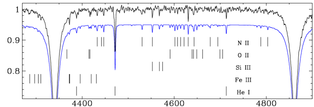
Figure 1: Top: zoom-in of the mean WHT spectrum with the NLTE fit and line identifications, demonstrating some of the stronger lines of heavier elements. The fit is offset for clarity.      Bottom: the mean spectrum from the WHT (bottom) and NOT, offset in flux for clarity.

From our new spectra of KIC 7668647 we solve the orbital radial-velocity amplitude, and derive a lower limit of the mass of the companion of the sdB star, which is most likely an unseen white dwarf. We use the average spectrum to study the atmospheric parameters in detail. We show that the orbital Doppler-boosting (or beaming) signal in the Kepler light curve as well as the light travel-time as probed by the sdB pulsations both lead to independent confirmations of the spectroscopic orbit solution. We extract 132 significant pulsational frequencies, and in the final sections of this paper we discuss pulsational period spacings and frequency splittings, aiming to identify the spherical-harmonic degree of the modes and to disclose the rotation period and inclination angle of the subdwarf in KIC 7668647.

2 Spectroscopic observations

Over the 2010, 2011, and 2013 observing seasons of the Kepler field we obtained altogether 30 spectra of KIC 7668647. Low-resolution spectra (R $\approx$ 2000 – 2500) have been collected using the 2.56-m Nordic Optical Telescope with ALFOSC, grism #16 and a 0.5 arcsec slit, and the 4.2-m William Herschel Telescope with ISIS, the R600B grating and 0.9–1.0 arcsec slit. Exposure times were 600 s at WHT, and ranging between 450 s and 900 s at the NOT. The resulting resolutions based on the width of arc lines is 1.7 Å for the WHT setup, and 2.2 Å for the setup at the NOT. See Table 6 for an observing log.

The data were homogeneously reduced and analysed. Standard reduction steps within IRAF include bias subtraction, removal of pixel-to-pixel sensitivity variations, optimal spectral extraction, and wavelength calibration based on arc-lamp spectra. The target spectra and the mid-exposure times were shifted to the barycentric frame of the solar system. The spectra were normalised to place the continuum at unity by comparing with a model spectrum for a star with similar physical parameters as we find for the target (see Sect. 2.2). The mean spectra from each of the telescopes are presented in Fig. 1.

2.1 Radial velocities and orbit solution

Radial velocities were derived with the FXCOR package in IRAF. We used the H$\gamma$, H$\delta$, H$\zeta$ and H$\eta$ lines to determine the radial velocities (RVs), and used the spectral model fit (see next section) as a template. For ALFOSC spectra the final RVs were adjusted for the position of the target in the slit, judged from slit images taken just before and just after the spectral exposure. See Table 6 for the results, with errors in the radial velocities as reported by FXCOR.

The errors reported by FXCOR are correct relative to each other, but may need scaling depending on, amongst other things, the parameter settings and the validity of the template as a model of the star. As our original orbital fit results in a $\chi^{2}$-value=0.48, the FXCOR errors seem to be overestimated by about 30%. This is consistent with the RMS found for the orbital fit of about 7.0 km s^-1. Therefore we scaled the FXCOR RV errors by a factor of 0.7 to derive the errors on the orbital parameters below.

Assuming a circular orbit we find an orbital period of 14.1742(42) d, with a radial-velocity amplitude of 38.9(1.9) km s^-1 for the subdwarf. See Table 1 for the complete parameter listing. The radial velocities and the derived solution are shown in Fig. 2. When fitting an eccentric radial-velocity curve the eccentricity is fit as $e$=0.056(64). We thus use a circular orbit throughout this paper.

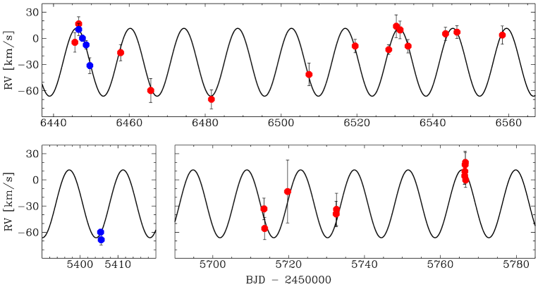
Figure 2: Radial-velocity curve from observations with the Nordic Optical (red dots) and William Herschel (blue dots) telescopes.

Given the solution presented in Table 1, the orbital radius of the sdB star can be approximated by $a_{\rm sdB}\sin i$ = 10.9(0.5) $R_{\sun}$, which corresponds to a light-travel time of 50.8(2.5) seconds between orbital phases corresponding to closest and furthest distance to the Sun.

The orbital solution combined with the mass function gives a lower limit for the mass of the companion of more than 0.40 $M_{\sun}$, if one assumes a canonical mass of 0.47 $M_{\sun}$ (see e.g. fontaine12) for the sdB star. The minimum distance between the two stars in this binary is then $a\sin i$ = 23 $R_{\sun}$. As the spectrum does not reveal clear evidence for light contribution from a companion, it should be either an unseen compact object, or an unseen M, K or G star. As the 2MASS J = 15.82(07) and H = 16.06(20) magnitudes do not indicate a rising infrared flux that would reveal the presence of a main-sequence star in this system, we conclude that the unseen companion is most likely a white dwarf. If the inclination of the system is smaller than $i$ $\la$ 30$\degr$ then the companion may be a neutron star or black hole ($i$ $\la$ 20$\degr$).

Table 1: Orbital solution of KIC 7668647 from RV measurements. $T_{\rm orb,RV}$ is the time at which the subdwarf is closest to the Sun in its orbit

system velocity [km s-1]	$-$27.4	(1.3)
radial-velocity amplitude $K$ [km s-1]	38.9	(1.9)
period $P$ [day]	14.1742	(0.0042)
$T_{\rm orb,RV}$ [BJD $-$ 2450000]	5974.76	(0.14)
reduced $\chi^{2}$	0.995
RMS [km s-1]	7.0

2.2 Atmospheric parameters

The spectra were shifted to remove the orbital motion, before being co-added to obtain high-S/N spectra (S/N $>$ 160) with minimal orbital line broadening, for both observatories. We derived the atmospheric parameters of the star from each of these mean spectra, and list average values of these parameters with errors as errors-in-mean, in Table 2. For this purpose we used the fitting procedure of edelmann03, with the metal-line blanketed local thermodynamic equilibrium (LTE) models of solar composition described in heber00. The errors on the final adopted values reflect the spread of the individual measurements rather than the formal errors. However, as the error-in-mean for the averaged helium/hydrogen abundance is unrealistically small we use the smaller of the two individual errors for our final value. Our final adopted LTE values are $T_{\rm{eff}}$ = 27700(300) K, $\log g$ = 5.50(3) dex and $\log\left(N_{\mathrm{He}}/N_{\mathrm{H}}\right)$ = $-$2.65(3) dex, which are quite consistent with the parameters $T_{\rm{eff}}$ = 27700 K, $\log g$ = 5.45 dex, $\log\left(N_{\mathrm{He}}/N_{\mathrm{H}}\right)$ = $-$2.5 dex found from an initial NOT survey spectrum in ostensen11b. Systematic errors related to model physics are typically of the order 500 K, 0.05 dex, and 0.05 dex, for $T_{\rm{eff}}$, $\log g$, and $\log\left(N_{\mathrm{He}}/N_{\mathrm{H}}\right)$, respectively.

Table 2: Atmospheric parameters of the subdwarf in KIC 7668647, derived from LTE spectral fits

Telescope	$T_{\rm{eff}}$	$\log g$	$\log\left(N_{\mathrm{He}}/N_{\mathrm{H}}\right)$
	K	cm s-2
NOT	27370(90)	5.470(13)	–2.654(28)
WHT	27990(70)	5.528(11)	–2.650(37)
adopted	27700(300)	5.50 (3)	–2.65(3)

Besides the lines of the hydrogen Balmer series and He i lines, clear lines of heavier elements are present. To quantify these, we fitted the mean WHT spectrum with the NLTE model atmosphere code Tlusty 204 (hubeny95) and performed spectral synthesis with Synspec 49 (lanz07). Our models included H, He, C, N, O, Si and Fe opacities consistently in the calculations for atmospheric structure and synthetic spectra. We fit the observed spectrum with the XTgrid fitting code (nemeth12). This procedure is a standard $\chi^{2}$-minimization technique, that starts with a detailed model and by successive approximations along the steepest gradient of the $\chi^{2}$ it converges on a solution. Instead of individual lines, the procedure fits the entire spectrum so as to account for line blanketing. However, the fit is still driven by the dominant Balmer lines with contributions from the strongest metal lines (listed in Table 7). We used a resolution of $\Delta\lambda=1.7$ Å and assumed a non-rotating sdB star.

The best NLTE fit was found with $T_{\rm{eff}}$ = 28 100 K and $\log g$ = 5.55 dex, using the Stark broadening tables of tremblay09. When using the line broadening tables from lemke97 alone we found a lower surface temperature and gravity, by about 860 K and 0.07 dex, respectively. A very similar systematic shift was found for the sdB star KIC 10553698 by ostensen14a.

Table 3: Parameters for the NLTE fit shown in Fig. 1, with solar abundance ratios from asplund2009 for comparison.

Parameter	Value	$+1\sigma$	$-1\sigma$	Unit	Solar
$T_{\rm{eff}}$	28100	1080	220	K
$\log g$	5.550	0.008	0.026	cm s-2
$\log n(\mathrm{He})/n(\mathrm{H})$	–2.57	0.03	0.07	dex	–1.07(1)
$\log n(\mathrm{C})/n(\mathrm{H})$	–5.00	0.40	0.40	dex	–3.57(5)
$\log n(\mathrm{N})/n(\mathrm{H})$	–4.14	0.09	0.13	dex	–4.17(5)
$\log n(\mathrm{O})/n(\mathrm{H})$	–4.59	0.24	0.30	dex	–3.31(5)
$\log n(\mathrm{Si})/n(\mathrm{H})$	–5.79	0.34	0.51	dex	–4.49(3)
$\log n(\mathrm{Fe})/n(\mathrm{H})$	–4.31	0.48	0.04	dex	–4.50(4)

Errors and abundances for the elements that were found to be significant are listed in Table 3. Statistical errors were determined by changing the model in one dimension until the critical $\chi^{2}$-value associated with the confidence limit at the given degree-of-freedom was reached. The resulting fit is shown together with the mean spectrum in Fig. 1.

Our NLTE model provides consistent parameters with the LTE analysis. We find that the abundances of Fe and N are about solar, whereas the other elements are depleted. This pattern agrees with the typical abundance profile of sdB stars (see e.g. geier13a). High depletion is normal in sdB stars due to gravitational settling, and large deviations from the solar mixture for individual elements are also common (heber00).

3 The orbital light curve from Kepler photometry

We analysed the Kepler light curve of KIC 7668647 as obtained in Kepler quarters Q06–Q17, totalling 2.88 year of data with 58.85 s sampling time ( i.e. short-cadence data; see gilliland10b). This photometric time series of 1.4 million data points spans BJD 2455372 to 2456424, which is roughly the same range as for our spectroscopic dataset. As for the similar sdBV+WD binary KIC 11558725 (telting12), we expect that part of the variability in the Kepler light curve could be due to orbital Doppler beaming.

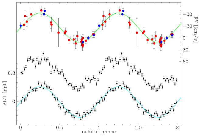
Figure 3: Bottom: the first half of the 2.8 year long Kepler light curve from quarters Q06 through Q16, folded on the orbital period and binned into 50 bins, with a model fit as listed in Table 4. Middle: folded second half of the light curve, offset by 0.3 ppt for clarity. The structure in this curve relates to imperfect detrending around gaps in the light curve. Top: phased radial velocities from the spectra from the Nordic Optical (red dots) and William Herschel (blue dots) telescopes

Table 4: Sine fits to parts of the orbital lightcurve of KIC 7668647 from Kepler measurements. $T_{\rm orb,B}$ is half an orbit before $T_{\rm orb}$ in Table 1. BJD values have 2450000 subtracted.

BJD range	# data	$A$ [ppt]	$P$ [d]	$T_{\rm orb,B}$ [BJD]	RMS [ppt]
5372.466 – 5626.812	330175	0.1658 (56)	14.081 (14)	5964.95 (47)	2.29
5626.813 – 5874.790	330178	0.1632 (55)	14.164 (15)	5967.84 (25)	2.20
5874.791 – 6139.383	330176	0.1514 (55)	14.234 (16)	5967.50 (09)	2.18
6139.384 – 6390.969	330179	0.1453 (56)	14.122 (16)	5968.88 (35)	2.25
5372.466 – 5874.790	660353	0.1625 (39)	14.1566 (52)	5967.61 (14)	2.25
5372.466 – 6390.969	1320708	0.1546 (28)	14.1666 (19)	5967.84 (04)	2.23

The 2.88 year coverage has 37 gaps in the data, with durations typically on the order of one day due to safing and repointing events, but including five prolonged periods ($\sim$5 to $\sim$15 days) void of data. The data typically needs detrending to account for instrumental offsets and drifts following data voids. Given that the binary period of KIC 7668647 is close to that of the spacing of the data gaps, we attempted to process the raw Kepler data in such a fashion to avoid any unnecessary loss of amplitude at the binary period.

First, we checked for possible contamination by neighbouring stars. Fortunately, the signal in the optimal aperture chosen by the standard pipeline is only slightly affected by that of other objects around our target (see the seasonal contamination described in the next subsection). This made the data processing less complex as we could avoid customization of the optimal aperture. Subsequently, we tried out fluxes from the pre-search data-conditioning (PDC) and simple aperture-photometry (SAP) apertures (jenkins10). The PDC fluxes were nicely detrended, however the data stitching implicitly removed the binary signal. As we could not use the PDC fluxes, we worked with SAP fluxes only, which however still needed to be corrected with some kind of detrending. For this purpose we used cotrending basis vectors (CBV). The PyKE (kinemuchi12) pipeline allows the implementation of a number of CBVs to approximate the systematics seen in the light curve. Often, we have to apply additional detrending by means of spline fitting to the residuals. In order not to affect the amplitude of the binary signal we skipped that step in this particular case, allowing some long-term instrumental variation to be present in our data. Finally, the data were 4.5$\sigma$ clipped to remove outliers and were transformed to fractional intensities $\Delta$I/I. The full light curve of 1.4 million points has a standard deviation $\sigma$=2245ppm . For the determination of the photometric orbital amplitude we only used the 1.32 million zero-flagged Kepler data points of Q06–Q16, with standard deviation $\sigma$=2235ppm .

We find that the applied trend correction works almost perfectly in the first half of the data set, but leaves obvious offsets around many data voids in the latter half of the data set. This may also be aggravated by possible deterioration of the CCDs over the lifetime of Kepler, and the lack of updated flatfields to account for this. In Fig. 3 we show the Kepler light curve folded on the orbital period into 50 phase bins, for both the first and second half of the data, showing that the latter folded curve shows significant deviations induced by imperfect detrending.

The level of detail to which this affects the determination of the photometric orbital amplitude is presented in Table 4, where we list the results of sine fits to parts of the processed Kepler data of KIC 7668647 . Here we divided the Q06–Q16 data set in 4 parts of equal number of data points. Whereas the amplitude at the orbital period is consistent for the first two quarters, it seems to decline in the last two quarters.

For this reason we use only the first half of the Kepler data to determine the photometric orbital parameters of KIC 7668647. A sine fit reveals the orbital period to be 14.1566(52) d, in agreement with the period found from spectroscopy, with amplitude of 162.5(3.9) ppm. We do not find orbital harmonics.

3.1 Doppler beaming

The high precision Kepler data permits us to accurately explore the low-amplitude Doppler beaming effect, something that is very hard to do with ground-based data. This effect is induced by stellar motion in a binary orbit and causes brightness modulation (RL79). The Doppler beaming effect permits an estimate of the radial velocity without resorting to spectroscopic data. A confirmation of the correspondence between Doppler beaming amplitudes, radial velocities, and the light-time effect, all in one object, was presented by telting12.

The light curve of KIC 7668647 displays a brightening of the sdB star at the orbital phases where the star is approaching us in its orbit (i.e. when its orbital radial velocities are negative, see Fig. 3), and this is exactly the effect expected by Doppler beaming. Note that unlike KPD 1946+4330 (bloemen11), KIC 7668647 does not show any sign of ellipsoidal deformation which in the closest sdB+WD binaries produces a strong signal at $P_{\rm{orb}}$/2 (see also e.g. silvotti12). This is consistent with the much longer orbital period of KIC 7668647 as opposed to the 0.4 d period of KPD 1946+4330.

In the case of Doppler beaming the observed flux from the target, $F_{\lambda}$, is related to the emitted spectrum, $F_{0,\lambda}$, and the projected orbital velocity, $v_{r},as$

$$F_{\lambda}=F_{0,\lambda}\left(1-B{v_{r}\over c}\right)$$ (1)

and the beaming amplitude relates to the orbital radial-velocity amplitude, $K$, as

$$A_{B}\leavevmode\nobreak\ D=B{K\over c}\leavevmode\nobreak\ ,$$ (2)

where $A_{B}$ is the amplitude of the beaming signal in the light curve (see Fig. 3), and $D$ the Kepler decontamination factor. The beaming factor $B$ is reflecting the relativistic aberration of the wavefront and the Doppler shift of the target spectrum within the Kepler wave band. It was computed for KIC 11558725 by telting12, following the procedure described in bloemen11. Here we adopt the same value $B$= 1.403(20), since KIC 11558725 and KIC 7668647 have very similar effective temperature and surface gravity.

The Kepler pixels onto which our target is imaged suffer from contamination from neighbouring objects, and from passing charge from brighter sources when clocking out the CCD. According to the Kepler Archive Handbook, the seasonal contamination factors for KIC 7668647 are 0.048, 0.067, 0.066, 0.041 or 0.0555 on average, implying that all periodic amplitudes derived from these Kepler fluxes should be multiplied by $D$ = 1/(1$-$0.0555) = 1.059 to get the intrinsic amplitudes of KIC 7668647.

We find that the photometric amplitude of the Doppler beaming as seen by Kepler and corrected for contamination, is consistent with the spectroscopically derived radial-velocity amplitude within the errors of the data. Given the observed amplitude $A_{B}$=163(4) ppm (Table 4), we use Eq. (2) to derive a value of $K$=36.8(1.1) km s^-1 for the orbital radial-velocity amplitude, from Doppler beaming.

The fact that this value is consistent with that of the spectroscopic value proves that the companion of the sdB does not significantly contribute to the observed Doppler beaming, consistent with a compact nature of the companion. Similarly, as the beaming fully accounts for the photometric variability at $P_{\rm orb}$, and no reflection-effect variability is observed, the companion must be of a compact nature.

4 The orbit derived from the light travel-time probed by the pulsations

In analogy to the effect that the Earth’s orbit has on arrival times of a variational signal, and on the apparent frequencies of that signal, the orbit of the sdB alters the phases and frequencies of its pulsations as perceived by a distant observer.

For the similar sdB+WD system KIC 11558725 (telting12) we have shown that it is possible to derive an independent orbital solution by using the pulsations as clocks to exploit the orbital light travel-time delays, equivalent to the method used by hulse75 for pulsars. If the orbit is not known, one can use the pulsations as clocks to derive the light-travel time that corresponds to the radius of the orbit, which relates to the radial-velocity amplitude $K$ that can be obtained from spectroscopy or the Doppler-beaming curve as

$$\Delta t_{\rm R}=\frac{a_{\rm sdB}\sin i}{c}=\frac{K}{c}\frac{P_{\rm orb}}{2\pi}\sqrt{1-e^{2}}\leavevmode\nobreak\ ,$$ (3)

where we introduce the Rømer delay, $\Delta t_{\rm R}$, to represent the light-travel time. For a circular orbit, the light-travel delay as a function of the subdwarf’s position in its orbit can be written as

$$T_{\rm delay}(t)=\Delta t_{\rm R}\leavevmode\nobreak\ \cos\left(\frac{2\pi}{P_{\rm orb}}(t-T_{\rm orb,R})\right)\leavevmode\nobreak\ ,$$ (4)

where $T_{\rm orb,R}$ is the time at which the subdwarf is closest to the Sun in its orbit, corresponding to that listed in Table 1.

We did not detect any second- or third-harmonic peaks, neither for the orbit nor for the pulsations. Hence, for sinusoidal signals the Kepler light curve of KIC 7668647 can be approximated by

$$\frac{\Delta I(t)}{I} = A_{B}\sin\left(\frac{2\pi}{P_{\rm orb}}(t-T_{\rm orb,B})\right)$$ (5)

$$+ \sum_{i}A_{\rm i,puls}\sin\left(2\pi F_{\rm i,puls}(t-T_{\rm i,puls}+T_{\rm delay}(t))\right)\leavevmode\nobreak\ ,$$

where the first term describes the orbital beaming effect, and where all individual pulsations are affected by the same orbital light-travel delay $T_{\rm delay}(t)$. Here, the phase of the individual pulsations, $T_{\rm i,puls}$, is expressed in the time domain rather than as an angle. Note that the above sum of sine curves is equivalent to the model that we fit as part of the prewhitening procedure described in the next section, with the addition of a phase delay that introduces just two extra parameters, i.e. the amplitude $\Delta t_{\rm R}$ and timing reference $T_{\rm orb,R}$ of the light-travel delay.

We apply the above Eq. (5) to derive a third independent measurement of the radial-velocity amplitude of the subdwarf in KIC 7668647. For this purpose we fitted the above model to the Kepler Q06–Q17 light curve. For the light-travel delay and corresponding timing zero point we use separate parameters from those representing the Doppler-boosting amplitude and timing zero point in the first term of Eq. (5), in order to make this determination of the orbital parameters truly independent from the Doppler-boosting value. In the model we included the 70 strongest frequencies of the subdwarf, with amplitude threshold of S/N $>$ 6.4. We repeated this using only the strongest 30 (S/N $>$ 9.4), and only the strongest 10 pulsations (S/N $>$ 38).

Table 5: Orbital light travel-time delay in KIC 7668647 from timing the pulsations

# of pulsations	$\Delta t_{\rm R}$	$T_{\rm orb,R}$
10	23.8 (3.8)	5975.31 (0.37)
30	25.6 (2.7)	5974.89 (0.24)
70	26.5 (2.5)	5974.95 (0.21)

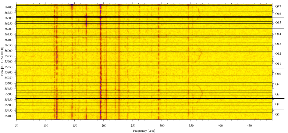
Figure 4: Dynamic Fourier spectrum from quarters Q06 through Q17 computed for 10 day stretches of data, versus BJD – 2400000. The frequency-variable feature at 365 $\mu$Hz is a spacecraft artefact (baran13). The dark horizontal lines reflect data gaps.

Simultaneously fitting all 70 pulsational amplitudes, frequencies and phases, together with the Rømer timing zero point and delay as free parameters, we find $T_{\rm orb,R}$=5974.95(21) [BJD – 2450000] and $\Delta t_{\rm R}$=26.5(2.5) s. The latter is equivalent to a value of $K$=40.8(3.8) km s^-1 for the orbital radial-velocity amplitude. Both the Rømer timing zero point and delay are in excellent agreement with the spectroscopic values in Table 1, and with those derived from the Doppler beaming. We note that the accuracy of the light-travel delay can be improved by using many pulsations in the model, even if they have amplitudes with only moderate S/N, as can be judged from Table 5.

5 The pulsation spectrum

After having used the pulsations as clocks to confirm the orbit, we here present the pulsation frequencies in KIC 7668647 in detail. We thereafter proceed to present mode identifications that will be useful input for a possible seismic study of KIC 7668647. In this paper we specifically aim to derive the rotation period of the star as a first seismic result.

For the determination of the pulsational signal in the Kepler light curve of KIC 7668647 we used the full Q06–17 data set described in Sect. 3, of in total 1.4 million points. The orbital light-time effect generates orbital sidelobes in the pulsational frequency spectrum (see e.g. SK12; telting12); for KIC 7668647 the amplitude of the orbital sidelobes are at the level of the noise in Fourier space. We opted to first transform the observation timings to remove the orbit, equivalent to the removal of Earth’s motion in the heliocentric timing correction. While this transformation removes the orbital sidelobes from the frequency peaks, it will also focus all power of the sidelobes into that of the main frequency peak, slightly enhancing the S/N of the intrinsic frequencies.

An iterative prewhitening process, involving an implementation of the fast-Fourier transform that allows for unevenly sampled data (see press1992, page 574) to find peaks, and subsequent non-linear least-squares (NLLS) sine-curve fits to subtract the pulsational content mode by mode from the original data, was used to derive the frequency list of Table 8. We extracted 132 significant frequencies, in addition to the orbital frequency.

We use the mean value of the Fourier amplitude spectrum of the original data to approximate the standard deviation on the amplitudes in Fourier space, $\sigma_{\rm FT}$=3.2 ppm. The mean value of the Fourier amplitude spectrum after removing the orbital and pulsational variations is still 3.2 ppm, which shows that the variance of the original data is dominated by measurement errors, and not by signal from our target. We adopt 4.5$\sigma_{\rm FT}$=14.4 ppm as the threshold of significance of the peaks in the Fourier amplitude spectrum. At the level of this 4.5$\sigma$ threshold we expect about 5 spurious peaks below the Nyquist frequency of 8500 $\mu$Hz, given the 1/$T$ resolution of 0.011 $\mu$Hz. Table 8 lists the 132 significant pulsation frequencies, with 16 other lower-significance frequencies that seem convincing-enough multiplet members to be listed (3.4 $<$ S/N $<$ 4.5).

The errors on the pulsational parameters as listed in Table 8 were obtained by fitting a non-linear multi-sine model, while using the standard deviation $\sigma$=2245 ppm of the Kepler data as an estimate of the measurement errors. This results in a reduced $\chi^{2}$ value of 0.94, with an RMS of 2180 ppm, and an estimate of the formal errors on the pulsation amplitudes of 2.6 ppm. The latter is somewhat smaller than our error estimate of 3.2 ppm based on the mean (residual) Fourier amplitude spectrum, and we have used the more conservative of the two error estimates to test the significance of individual peaks, and for the S/N column in Table 8. We stress that for many of the modes the amplitude variability is larger than the formal errors on their fitted amplitude.

We note that the observed amplitudes in Table 8 have neither been corrected for the Kepler decontamination factor $D$=1.059 (see Sect. 3), nor for amplitude smearing due to the effective exposure time of 58.85 seconds. Both effects cause the observed amplitudes to be smaller than the intrinsic amplitudes. The latter affects mostly the shortest periods ($p$-modes): for the shortest detected periods of 211 seconds the observed amplitude is reduced by 12%.

It is clear from Table 8 that most pulsation frequencies lie in the $g$-mode domain, while only few low-amplitude $p$ modes are present in KIC 7668647. Most pulsations are not stable over time, which causes prewhitening to be difficult, and which otherwise manifests itself as a bunch of narrow peaks around most of the pulsation peaks in the Fourier spectrum (see Figs. 5, 6, 9). To investigate for each pulsation the magnitude of any amplitude or frequency variations, we list the amplitudes of the pulsations for the first and second half of the data set, fitted while keeping fixed frequencies. The resulting amplitudes are listed in Table 8.

To illustrate the fact that most strong pulsation modes are present throughout the Kepler run, we show a section of the Fourier transform in a dynamic form in Fig. 4. The multiplets show clear beating patterns in this figure. It appears that some modes are relatively stable throughout the 3 years of Kepler monitoring, while other modes show significant amplitude variability on timescales comparable to or even longer than the duration of the Kepler run. This is in contrast with the much shorter $\sim$60 day timescale of the amplitude variability of the stochastic pulsations seen in KIC 2991276 (ostensen14b).

On the other hand there are many modes in KIC 7668647 that show amplitude variability with prolonged periods where the mode is not excited. Some modes are of short-lived nature, with life times comparable to the rotation period (see Sect. 6); some permanently present modes have short-lived episodes of high amplitude.

6 Pulsational period spacings and multiplet splittings, rotation and inclination

Recently, reed11c have revealed that $g$-modes in sdB stars show sequences with near-constant period spacings. As the period spacings follow the asymptotic relation for $g$-modes, the spacings relate to the value of the spherical-harmonic degree $\ell$ of the modes, and hence allow us to determine the $\ell$-value of the modes directly. reed11c already identified $\ell$ values for the $\sim$20 pulsations that could be resolved in the Kepler survey data of KIC 7668647. They identified an $\ell$=1 sequence with period spacing $\Delta\Pi_{\ell=1}$=248 s, and an $\ell$=2 sequence with period spacing $\Delta\Pi_{\ell=2}$=145 s, with a ratio close to the theoretically expected $\sqrt{3}$. For the modes identified through the period sequence the radial order $n$ can be determined directly, save for a zero-point offset that has to be modelled. For our identification of the radial order $n$ of the modes in Table 8 we set the zero-point to modes with periods that satisfy $P\sqrt{\ell(\ell+1))}\sim$800 s (see charpinet02).

To the first order in the rotation frequency $\Omega$, the observed frequencies of the modes are altered by $m\Omega(1-C_{n\,\ell})$, with $m$ the azimuthal quantum number of the spherical harmonic. Hence, for non-radial modes of given degree $\ell$, we expect frequency multiplets of 2$\ell$+1 peaks to occur. In the asymptotic regime, the value of $C_{n\,\ell}$ can be approximated by 0 for $p$-modes, and by $1/(\ell(\ell+1))$ for high-$n$ $g$-modes. The latter implies a value of $C_{n\,\ell}$$\sim$0.5 and $C_{n\,\ell}$$\la$0.17 for $\ell$=1 and $\ell$¿1 $g$-modes, respectively.

The (multiplet) frequency splittings we discuss below are derived by taking the frequency difference of subsequent entries in the sorted frequency list in Table 8.

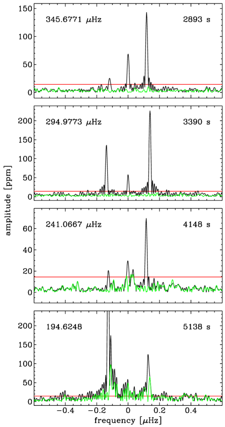
Figure 5: Top: DFT window function of the Q06–Q17 data set.     Bottom panels: Complete and resolved $\ell$=1 triplets in the Fourier Transform of the Q06–Q17 data set. The prewhitened FT is overdrawn (green); for the central mode in the lowest panel no prewhitening was attempted prompted by the amplitude-variable nature of this triplet. The red horizontal line marks the 4.5 $\sigma$ limit. The triplet spacings are 0.12–0.14 $\mu$Hz.

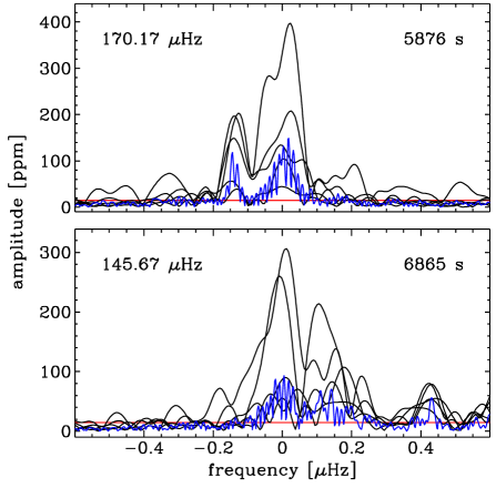
Figure 6: Wide-peaked $\ell$=1 doublets in the Fourier Transform of the Q06–Q17 data set (blue). The black curves are FTs of the five $\sim$210-day subsets of the data, which show the amplitude variability of these modes. The red horizontal line marks the 4.5 $\sigma$ limit. The doublet spacings are consistent with those in Fig. 5.

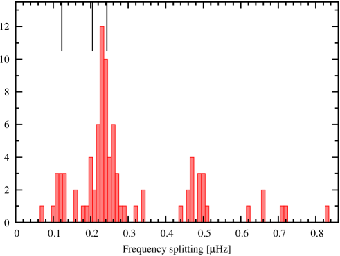
Figure 7: Histogram of frequency splittings listed in Table 8, that are determined by taking the frequency difference between subsequent entries in the sorted frequency list. The vertical indicators at 0.123 $\mu$Hz, 0.205 $\mu$Hz, and 0.243 $\mu$Hz, reflect expected $\ell$=1, 2, 8 splittings for a rotation period of 47 days. The splittings at 0.13 $\mu$Hz are identified as $\ell$=1, and the peak at 0.23 $\mu$Hz as $\ell$$\geq$2 modes.

6.1 Mode identification: $\ell$=1

As a base-line observation for mode identification in KIC 7668647 we use the set of four $g$-mode triplets with narrow frequency splittings of 0.12–0.14 $\mu$Hz, displayed in Fig. 5. These are the only triplets with such narrow splitting in KIC 7668647. All four triplets are consistent with the $\ell$=1 period spacing sequence, and all have at least one frequency peak that is among the strongest peaks in KIC 7668647.

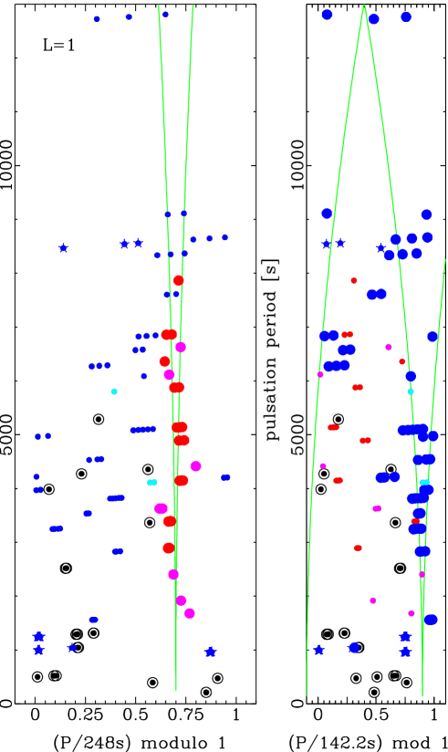
Figure 8: Echelle diagrams of the $\ell$ = 1 (left) and $\ell$ = 2 (right) period-spacing sequences. Green curves reflect the full width of $\ell$ = 1 (left) and $\ell$ = 2 (right) multiplets. Red dots are secure $\ell$=1 identifications from frequency splittings; magenta dots are likely $\ell$=1 identifications based on period spacing. All dark blue symbols reflect modes that have frequency splittings corresponding to $\ell$$\geq$2. Blue stars correspond to modes in $\ell$$\geq$3 multiplets. Cyan dots are likely $\ell$=2 identifications based on period spacings only. Ringed dots are modes that could not be classified with any certainty.

Accepting these triplets as $\ell$=1 modes, the frequency splitting immediately discloses a rotation period between 41 and 48 days, assuming $C_{n\,\ell}$=0.5 . The observed $\ell$=1 triplet frequency splitting also implies that multiplet splittings for modes with higher $\ell$ values can range between 0.20–0.28 $\mu$Hz assuming $C_{n\,\ell}$$\la$0.17 . In Fig. 7 we show a histogram of the multiplet splittings listed in Table 8; the histogram clearly shows an abundant presence of higher-$\ell$ splittings peaking at 0.23 $\mu$Hz, which is consistent with those implied by the observed $\ell$=1 splitting.

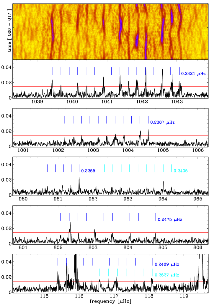
Figure 9: Selected regions in Fourier space where large multiplets occur, indicative of $\ell$$>$2. The Fourier amplitudes are given in units of ppt; the red line reflects our adopted detection limit. For each apparent sequence of modes, a grid of vertical lines is drawn with an indicated average splitting based on the frequencies of the first and last clear mode in the sequence. The bottom panel shows either a chance alignment of an $\ell$=2 and an $\ell$=3 multiplet, or a single multiplet of $\ell$$\geq$6. The 802–805 $\mu$Hz structure could be an $\ell$$\geq$6 multiplet. The 1002–1004 $\mu$Hz structure could be an $\ell$$\geq$5 multiplet. For the 1039–1043 $\mu$Hz structure, which is consistent with an $\ell$$\geq$8 multiplet, the dynamic Fourier transform as a function of time is shown; for this a sliding window of 200 days was used. Note that all frequency splittings of these $\ell$$>$2 modes are very similar in value.

In Table 8 we list more $\ell$=1 identifications, some among the highest-amplitude peaks in the Fourier spectrum, that were identified from the period-spacing sequence anchored by the 4 triplets in Fig. 5. Following the period-spacing sequence, we discovered in the FT a number of likely $\ell$=1 modes that have broad peaks that reflect short-lived episodes of very high amplitude. An example of such a mode is the 145.71 $\mu$Hz mode labelled f₅ in baran11b, which was the strongest mode in the initial 30 days of Kepler survey data, but is only seen at high amplitude in the very beginning and very end of the Q06-Q17 observations. In Fig. 6 we present examples of these extreme amplitude-variable $\ell$=1 modes, where the full data set has been divided into 5 near-equal chunks to bring out the Fourier amplitude variability. These wide $\ell$=1 peaks are found at low frequencies: strong ones at 145.67 and 170.17  $\mu$Hz (see Fig. 6), and weak but detectable ones at 127.14 and 157.23  $\mu$Hz.

The clear $\ell$=1 period spacing sequence is presented in echelle format in Fig. 8, where we used the spacing $\Delta\Pi_{\ell=1}$=248 s to fold the periods. Unlike for the sdB+WD binary KIC 10553698 (ostensen14a), the pulsations in KIC 7668647 are not excited for many subsequent values of the radial order $n$. Although for radial orders $\sim$4–25 (periods 1650–6900 s) the sequence is followed quite well, the longest continuous string of excited $\ell$=1 modes is only 5 orders long: orders $\sim$21–25 (see Table 8). Hence it is not feasible to conclusively identify trapped modes (charpinet02; ostensen14a), from the $\ell$=1 and $\ell$=2 period sequences in KIC 7668647. Note however, that there are modes that do not fall on either of these period sequences (see Fig. 8), and these may be either trapped $\ell$=1 or $\ell$=2 modes or modes with even higher degree $\ell$. The only high-amplitude modes among these are all shown in Fig. 9 and may all be part of high-degree multiplets.

6.2 Mode identification: $\ell$=2

As will be shown below, there is strong evidence for a few multiplets of more than 5 components in KIC 7668647. As the frequency splitting for all $\ell$$\geq$2 degree multiplets is expected to be similar, and because $\ell$$>$2 multiplets are observed, it is inconclusive to label a quintuplet with an $\ell$=2 origin, as it could be an incomplete multiplet of higher degree.

In the right-hand panel of Fig. 8 we show the echelle diagram for a folding period of 142.2 s, which is close to the theoreticaly expected $\Pi_{\ell=1}/\sqrt{3}$=143.2 s period spacing. In Table 8, we list the most likely $\ell$=2 modes, based on frequency splitting and period spacing. A group of 9 multiplets clearly matching the period spacing is found for periods between 2800–5100 s (radial orders 17–33), although the longest continuous string of excited $\ell$=2 modes is only 3 orders long. Note that in Figure 8 we denote the $\ell$$\geq$3 multiplets with star symbols.

6.3 Curiosity cabinet: modes with degree $\ell$$\geq$3

Even though high-degree modes have low visibility due to cancellation effects on the stellar disk, there is strong evidence that such modes are visible in KIC 7668647 to the sensitive eye of the Kepler spacecraft. dziem77 and SW81 list the cancellation factors as a function of $\ell$ for certain choices of the limb-darkening law. Photometric observability of modes with degrees 4$\leq$$\ell$$\leq$8 is expected to drop by two orders of magnitude with respect to that of $\ell$=1 modes. In case the photometric variability has a significant component due to surface-gravity effects, the drop may be only of one order of magnitude. As the highest $\ell$=1 amplitudes in KIC 7668647 are around 400 ppm, intrinsically strong high-$\ell$ modes may just be detectable by Kepler.

In Figure 9 we show 5 frequency ranges in which we find evidence for 3$\leq$$\ell$$\leq$8 multiplets in KIC 7668647. None of these multiplets is fully complete, but in some only few components are missing. All these high-$\ell$ multiplets show the frequency splitting of 0.239–0.253 $\mu$Hz. At 1002–1005 $\mu$Hz we find an $\ell$=6 multiplet, with most peaks barely at the detection limit, but which is nonetheless a convincing multiplet due to the distinct pattern of the peaks. At 1039–1043 $\mu$Hz we find an $\ell$=8 multiplet, with 11 clearly detected modes, and an average splitting of 0.242 $\mu$Hz. As for these high-$\ell$ modes the value of $C_{n\,\ell}$ is expected to be close to zero, the rotation period we derive from the splittings ranges between 45.7–48.4 d.

We also show a dynamic Fourier transform of the 1039–1043 $\mu$Hz region, based on 200-day chunks of Kepler data. This diagram shows that both amplitudes and frequencies are not stable over time. The individual splittings between subsequent components change over time, and only through the extensive length of the data set can accurate average splittings be determined. Like some of the $\ell$=1 modes, some modes in these high-$\ell$ multiplets are relatively short lived. It seems that to find the missing components of the multiplets Kepler should have performed on the same field for only a bit longer.

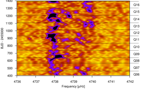
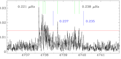
Figure 10: The $p$-mode complex at 4739 $\mu$Hz. Top: dynamic Fourier transform computed with a running window of 50 days. The colour cuts range from 0 to 0.08 ppt. Bottom: FT of the full Q06–Q17 Kepler light curve, with the 6 modes that are listed in Table 8 indicated by green vertical line segments, and the adopted detection threshold by the horizontal line. The typical 0.22-0.24 $\mu$Hz splitting is indicated for two pairs of these. Two more such splittings, involving less significant peaks, are indicated in blue. The broad power humps in the full-length FT reflect the short life times of these modes.

6.4 Radial rotation profile and $p$-modes

So far in this section we have assumed that the star has rigid rotation. In case of a non-rigid radial rotation profile, $\Omega(r)$, the multiplet splittings may be expected to vary along with the radial order of the pulsations, as different parts of the stellar interior are probed through pulsations of different radial order. Similarly, the splittings of $p$-modes reflect the rotation frequency in the outer envelope, whereas the $g$-mode splittings are a measure of the rotation frequency further inwards, probing all the way in to the base of the He mantle, outside the He-burning convective core. See e.g. charpinet00; charpinet14 for pulsation mode propagation as a function of stellar radius.

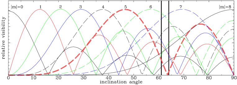
Figure 11: Relative visibility of $\ell$=8 modes as a function of inclination angle. Between $i$$\sim$61$\degr$ and $i$$\sim$64$\degr$ the $m$=0 and $|m|$=5 components have low visibility, while the other multiplet components are visible, similar to what is observed (see top panels of Fig. 9).

In the typical sdB $p$-mode region with periods shorter than 15 minutes we only find 5 scattered low but significant peaks in the region of 1900–2600 $\mu$Hz, and several more in a complex pattern of peaks at 4739 $\mu$Hz. For the modes in this complex pattern we present a dynamic Fourier diagram in Fig. 10, for which we have used chunks of 50 days to compute the running FTs. The figure shows that the modes in this pattern are short lived, with life times on the same order as the rotation period. Among the splittings between subsequent peaks, as listed in Table 8, we find two that have the usual values of 0.22–0.24 $\mu$Hz, and we find another two such splittings that involve two less-significant peaks (see Fig. 10). With a $p$-mode value of $C_{n\,\ell}$$\sim$0, the splittings as indicated in the figure correspond to a rotation-period range of 49–52 d, i.e. a similar but slightly longer rotation period as derived from the $g$-modes, implying a constant or slightly decreasing rotation frequency as a function of radius. We note, however, that the $p$-mode frequencies are few, and are difficult to interpret, with no observational anchor points such as clear multiplets to hold on to.

Another clue towards differential rotation may be presented by the different values of the rotational splitting of the $\ell$=1 triplets presented in Fig. 5. These triplets are placed in a narrow range of radial order, but their splittings differ from triplet to triplet. The largest difference is between the triplet at 345.7 $\mu$Hz, with radial order $n$=9 and splitting of 0.118 $\mu$Hz, and that at 295.0 $\mu$Hz, with radial order $n$=11 and splitting of 0.139 $\mu$Hz. When assuming rigid rotation, this difference corresponds to a difference in $C_{n\,\ell}$ values of almost 18%, which is large for what one may expect for high-$n$ $g$-modes (see e.g. charpinet00), and may in itself be evidence for non-rigid rotation.

6.5 Inclination angle

Even though many multiplets are incomplete, there are some that provide us information about the inclination angle of the star. In general, mode visibility is a function of inclination angle, and for some inclination angles that are close to modal node lines, particular modes in multiplets are not expected to be visible.

When taken all together, the $\ell$=1 triplets in Fig. 5 show that the central $m$=0 components are not as strong as the $|m|$=1 components, which points at an inclination angle larger than 45$\degr$, but not close to 90$\degr$.

Secondly, the $\ell$=8 multiplet shown in Fig. 9 can be interpreted as having a very low amplitude $m$=0 component at 1041.1 $\mu$Hz, and similarly low $|m|$=5 components. To simulate the expected visibility of an $\ell$=8 multiplet as a function of inclination angle we adapted the model described by schrijvers1999, that was originally used for modelling of pulsational line-profile variations. We assume that the brightness variation along the stellar surface can be described by a spherical harmonic with sinusoidal amplitude as a function of time. The result of this exercise is shown in Fig. 11, and one can infer that for an inclination angle close to $i$$\sim$62$\degr$ the $m$=0 and $|m|$=5 components have low visibility, while the other components are better visible. In case the observed structure reflects an $\ell$=9 multiplet instead, a similar constraint on the inclination angle can be derived: $i$$\sim$55$\degr$.

For an orbital inclination of $i$$\sim$62$\degr$ , which implies spin-orbit alignment, the orbital RV solution (Table 1) constrains the mass of the WD companion to 0.48 $M_{\sun}$, if one assumes a canonical mass of 0.47 $M_{\sun}$ for the sdB.

7 Summary and Conclusions

From our new low-resolution spectroscopy and the Kepler lightcurve we discovered that KIC 7668647 is a binary consisting of a B subdwarf and an unseen companion, likely a white dwarf. We found a circular orbit with $P_{\rm orb}$=14.2 d, and a radial-velocity amplitude of 39km s^-1.

The 2.88 years of short-cadence Kepler data of KIC 7668647 reveal Doppler beaming at the 163 ppm level. The light-travel delay measured by timing of the pulsations was derived at 27 s. Both the observed amplitude of the Doppler beaming and the measured light-travel delay are consistent with the spectroscopic orbital radial-velocity curve. The Doppler-beaming amplitude and the lack of the reflection effect both imply an unseen compact companion.

From the high signal-to-noise average spectrum we redetermined the atmospheric parameters of the subdwarf: $T_{\rm{eff}}$ = 27 700 K and $\log g$ = 5.50 dex (LTE values). Nitrogen and iron have abundances close to the solar values, while helium, carbon, oxygen and silicon are underabundant relative to the solar mixture.

We extracted 132 significant pulsation frequencies from the Kepler light curve, with strong evidence for additional pulsational content near the detection limit. We found several $p$-modes, and many frequencies in the $g$-mode domain, demonstrating the potential for a seismic analysis of this star. Many, if not all, of the pulsation modes show amplitude variability. For $\ell$=1 multiplets at low frequencies, 127–170 $\mu$Hz, some modes of high amplitude have short-lived epochs of very high amplitude, i.e. with a duration of a few times the rotation period. Many other modes of higher $\ell$ were found to be short lived, with the shortest life times comparable to the rotation period.

Long- and short-term amplitude variability has been observed in other sdB stars as well, see e.g. reed07b and ostensen14b who document also frequency and phase variability of sdB-star pulsations. These variations point at structural variability of the pulsation cavities and/or redistribution of pulsation energy over different modes. The above authors suggest that phase variability may originate in convective motions, which are somehow interacting with the Z-bump driving mechanism. The long time base observations of KIC 7668647 that we present here confirm that amplitude variability is indeed an important phenomenon in sdB-star pulsations.

We used four clear $\ell$=1 triplets to anchor the period-spacing sequences. We showed that many of the pulsation frequencies match period spacings of $\ell$=1 and $\ell$=2 sequences, with no obvious evidence for mode trapping. These period-spacing sequences will aid in the identification process of the modes in a future seismic study of this object. From these sequences we identify many $\ell$=1 $g$-modes in the range of radial orders $n$$\sim$4–29, and $\ell$=2 $g$-modes within $n$$\sim$17–61.

We find many multiplets, and many have amplitude-variable components. The long time base of the Kepler observations allows us to see many multiplet components, even though they are not all excited at the same time. Nevertheless, in spite of the extensive time coverage many multiplets remain incomplete.

There are several frequency regions that show multiplets of high-degree $\ell$$\geq$3 modes. As for the low-degree multiplets in KIC 7668647, all are incomplete or have low-amplitude components. Even though some of these components are below the 4.5-$\sigma$ detection limit, the patterns of equally-split frequencies are striking and make the detection of these high-$\ell$ multiplets quite reliable. The most convincing of these multiplets is indicative of modes with degree $\ell$=8, which is a novelty in observational sdB-star seismology.

Given that the surface cancellation effects in photometry are high, these high-degree modes must be intrinsically strong in KIC 7668647. For other types of pulsating stars with rapid rotation, high-degree modes are typically found from time-resolved spectroscopy: the stellar surface is resolved through rotational broadening of the absorption lines, which allows Doppler imaging. An example of a star with a dominant $\ell$=8 mode is the $\beta$ Cephei variable $\omega^{1}$ Sco (telting1998; berdyugina2003), showing clear spectroscopic variability, while because of its photometric stability the star was one of the prime standard stars of the Walraven photometric system. Although recent space missions have shown very dense pulsation spectra in different types of stars, we are unaware of any star for which an $\ell$=8 multiplet has been identified from photometry until now.

From mode-visibility considerations we derive that the inclination of the rotation axis of the sdBV in KIC 7668647 must have an intermediate value around $\sim$60$\degr$.

From the $g$-mode multiplet splitting we derive a rotation period of 46–48 d for KIC 7668647, at the inner depths of the He mantle sampled by these modes. The few, and difficult to interpret, $p$-mode splittings may point at a somewhat slower rotation rate further out in the envelope. Additional evidence for non-rigid rotation may come from the large difference between the splittings of the four main $\ell$=1 triplets. Detailed modelling of the observed splittings of the modes spanning almost 60 radial orders (e.g. beck2012), has the potential to reveal further evidence for non-rigid rotation in this star.

As in all sdBV binaries in the Kepler field studied so far, the rotation is subsynchronous with respect to the orbit. In this respect, and this holds also for the main atmospheric and the orbital parameters, KIC 7668647 lives in the same observable parameter space as KIC 11558725 (telting12).

KIC 7668647 is the third sdB pulsator in the Kepler sample with a confirmed compact stellar-mass companion. KIC 7668647 has the fifth-longest orbital period of all known sdB stars with compact companions, which is at the long end of the period range of the $\sim$100 known sdB binaries that have periods compatible with the common-envelope ejection scenario.

Assuming a canonical sdB mass of 0.47 $M_{\sun}$, we derived a lower limit for the mass of the companion of 0.40 $M_{\sun}$. The distance between the two companions is $\ga$23 $R_{\sun}$, which implies that if the sdB is a result of a common-envelope phase the progenitor must have been close to the maximum radius for a red giant, near the tip of the red-giant branch.

Appendix A Tables: measured radial velocities, fitted metal lines, and extracted frequencies with mode identifications

Table 6: Log of the low-resolution spectroscopy of KIC 7668647 and the RV measurements

Mid-exposure Date	Barycentric JD	S/N	RV	RVerr	Telescope	Observer/PI
	–2450000		km s-1	km s-1
2010-07-27T22:33:49.8	5405.44261	85.4	$-$59.9	2.4	WHT	JHT,CA
2010-07-28T01:46:03.9	5405.57610	84.0	$-$68.6	6.0	WHT	JHT,CA
2011-06-01T00:09:55.7	5713.50851	62.7	$-$33.2	12.4	NOT	JHT
2011-06-01T04:32:37.3	5713.69094	50.7	$-$55.7	12.8	NOT	JHT
2011-06-07T05:38:55.6	5719.73717	18.9	$-$13.3	35.9	NOT	JHT
2011-06-20T00:47:24.7	5732.53504	48.9	$-$39.0	14.6	NOT	JHT
2011-06-20T03:04:04.2	5732.62995	42.7	$-$33.8	18.5	NOT	JHT
2011-07-23T21:41:22.0	5766.40619	61.6	4.6	9.6	NOT	JHT
2011-07-23T23:11:50.8	5766.46902	49.1	9.8	13.6	NOT	JHT
2011-07-24T00:52:21.8	5766.53883	48.3	17.4	15.3	NOT	JHT
2011-07-24T02:32:25.2	5766.60831	58.2	20.1	11.1	NOT	JHT
2011-07-24T03:52:13.3	5766.66373	52.4	$-$0.0	8.4	NOT	JHT
2013-06-02T03:40:12.2	6445.65459	76.5	$-$4.6	11.3	NOT	JHT
2013-06-03T03:32:11.5	6446.64906	60.4	10.2	6.9	WHT	SM,TK
2013-06-03T03:45:30.7	6446.65831	60.9	16.5	8.0	NOT	JHT
2013-06-04T03:30:49.1	6447.64814	67.5	0.1	3.6	WHT	SM,TK
2013-06-05T03:01:42.6	6448.62795	77.9	$-$7.4	4.9	WHT	SM,TK
2013-06-06T02:07:07.8	6449.59008	69.6	$-$31.2	9.0	WHT	SM,TK
2013-06-14T05:02:21.6	6457.71198	78.0	$-$16.4	9.2	NOT	JHT
2013-06-22T03:19:35.4	6465.64078	61.0	$-$59.7	13.6	NOT	JHT
2013-07-08T03:33:28.0	6481.65065	60.3	$-$69.9	10.7	NOT	JHT
2013-08-02T20:57:10.9	6507.37547	37.5	$-$41.4	12.8	NOT	JHT
2013-08-15T00:49:00.7	6519.53630	61.6	$-$8.8	7.7	NOT	JHT
2013-08-23T20:58:37.2	6528.37614	46.9	$-$12.9	5.4	NOT	JHT
2013-08-25T20:51:56.3	6530.37145	75.0	13.9	12.9	NOT	JHT
2013-08-26T21:00:01.3	6531.37704	75.8	9.7	10.0	NOT	JHT
2013-08-28T23:26:33.5	6533.47875	70.1	$-$8.9	7.6	NOT	JHT
2013-09-07T20:30:43.9	6543.35638	47.2	5.2	7.5	NOT	JHT
2013-09-10T21:02:03.8	6546.37804	62.9	7.1	7.4	NOT	JHT
2013-09-22T20:10:49.5	6558.34205	67.6	3.8	10.3	NOT	JHT

Table 7: Fitted metal lines with equivalent widths larger than 50 mÅ.

Ion	Wavelength	$W_{\lambda}$	Ion	Wavelength	$W_{\lambda}$
	[Å]	[mÅ]		[Å]	[mÅ]
He i	3819.603	123.7	N ii	4227.736	77.1
He i	3819.614	54.5	N ii	4237.047	66.3
He i	3888.605	106.1	N ii	4241.755	59.8
He i	3888.646	126.1	N ii	4241.786	79.7
He i	3888.649	150.6	N ii	4432.736	64.8
He i	3964.729	61.6	N ii	4442.015	65.6
He i	4026.187	144.1	N ii	4447.030	91.9
He i	4026.187	53.2	N ii	4530.410	72.1
He i	4026.198	53.2	N ii	4552.522	64.1
He i	4026.199	98.9	N ii	4601.478	74.5
He i	4026.358	73.1	N ii	4607.153	66.6
He i	4143.761	76.5	N ii	4621.393	65.7
He i	4387.929	89.0	N ii	4630.539	114.0
He i	4471.473	207.5	N ii	4643.086	82.9
He i	4471.473	102.7	N ii	4678.135	83.7
He i	4471.485	102.7	N ii	4803.287	52.1
He i	4471.488	177.1	N ii	5001.134	93.9
He i	4471.682	127.0	N ii	5001.474	107.9
He i	4713.139	88.3	N ii	5005.150	117.0
He i	4713.156	52.2	N ii	5007.328	78.4
He i	4921.931	188.2	N ii	5045.099	75.3
He i	5015.678	151.3	O ii	4072.153	68.1
N ii	3955.851	59.3	O ii	4349.426	63.8
N ii	3994.997	109.0	O ii	4641.810	55.8
N ii	4035.081	73.7	O ii	4649.135	55.3
N ii	4041.310	89.2	Si iii	4552.622	66.8
N ii	4043.532	82.2	Si iii	4567.840	55.0
N ii	4082.270	53.2	Fe iii	4164.731	51.6
N ii	4176.159	71.4	Fe iii	5156.111	55.7

Table 8: Extracted pulsation frequencies. Three amplitudes are listed, based on multi-sine fits: the full Q06–17 amplitude, with errors of 2.6 ppm , and the amplitudes A and B of the first and second halves of the data, with error 3.8 ppm. For the S/N column we used the error estimate of 3.2 ppm based on the mean (residual) Fourier amplitude. Frequency differences, or splittings, between subsequent table entries are listed when smaller than 4.5 $\mu$Hz. Radial orders are listed for modes belonging to the $\ell$=1 and $\ell$=2 period sequences. Vertical arrows and horizontal delimiters indicate the multiplet ranges, with the radial order listed for the multiplet component that best matches the central component.

Frequency			Period		Ampl	S/N	Ampl A, B		Splitting	$n_{\ell=1}$	$n_{\ell=2}$
$\mu$Hz			s		ppm		ppm		$\mu$Hz
4.	8378	0.0007	206705	30	23	7.3	14	32
35.	0779	0.0011	28507.9	0.9	15	4.8	11	19
40.	1130	0.0011	24929.6	0.7	14	4.5	17	11	0.239
40.	3524	0.0007	24781.67	0.43	23	7.2	20	25
78.	0709	0.0009	12808.87	0.14	19	6.0	18	19	0.276
78.	3471	0.0006	12763.71	0.10	27	8.6	27	27	0.244
78.	5909	0.0007	12724.13	0.11	23	7.3	32	14
109.	7497	0.0010	9111.64	0.08	16	5.2	12	21	0.241		$\uparrow$
109.	9911	0.0008	9091.65	0.06	21	6.7	25	17			61
115.	3917	0.0006	8666.132	0.048	25	8.0	26	24	0.254		$\uparrow$
115.	64534	0.00042	8647.128	0.031	39	12.3	26	52	0.267
115.	91265	0.00012	8627.186	0.009	139	43.5	128	151	0.920		58
116.	8322	0.0008	8559.29	0.06	19	6.2	20	20	0.233
117.	0650	0.0008	8542.26	0.06	21	6.6	27	14	1.043
118.	1078	0.0008	8466.84	0.06	20	6.3	28	15	1.389
119.	49731	0.00008	8368.389	0.006	202	63.3	228	176	0.246		56
119.	74315	0.00009	8351.208	0.007	174	54.4	98	252	0.236
119.	97911	0.00011	8334.784	0.008	144	45.2	158	130			$\downarrow$
127.	1452	0.0006	7865.024	0.036	27	8.7	27	27	4.192	29
131.	33672	0.00048	7614.017	0.028	33	10.5	41	27	0.196
131.	5328	0.0008	7602.664	0.047	20	6.3	18	22
145.	67445	0.00014	6864.622	0.007	116	36.4	70	162	0.138	25
145.	81287	0.00019	6858.105	0.009	87	27.3	102	63	0.289	$\downarrow$
146.	10222	0.00027	6844.523	0.013	61	19.1	65	53	0.236		$\uparrow$
146.	33824	0.00046	6833.484	0.021	35	11.1	43	27	0.211
146.	5493	0.0008	6823.642	0.038	19	6.2	10	22	4.337		45
150.	88592	0.00042	6627.524	0.019	38	12.1	42	36	1.073	24
151.	9591	0.0007	6580.720	0.030	23	7.5	32	14	0.208
152.	1670	0.0007	6571.726	0.032	22	6.9	16	28
157.	23424	0.00049	6359.938	0.020	33	10.3	25	40	1.768	23
159.	0026	0.0006	6289.206	0.024	26	8.3	39	14	0.254		$\uparrow$
159.	2571	0.0006	6279.156	0.025	25	8.1	26	24	0.237
159.	4943	0.0010	6269.816	0.037	17	5.4	21	13	3.975		41
163.	4696	0.0010	6117.347	0.036	17	5.3	23	10	0.837	22
164.	3066	0.0006	6086.183	0.023	26	8.2	12	41			40
170.	02516	0.00015	5881.482	0.005	112	35.2	71	159	0.163	21
170.	18782	0.00011	5875.8610	0.0038	150	47.1	110	195	2.179	$\downarrow$
172.	3668	0.0007	5801.583	0.023	23	7.5	37	11			38
189.	1709	0.0006	5286.226	0.017	27	8.5	20	34
194.	498567	0.000039	5141.4260	0.0010	420	131.4	450	386	0.125	$\uparrow$
194.	62319	0.00048	5138.134	0.013	34	10.7	49	22	0.128	18
194.	75097	0.00012	5134.7627	0.0033	131	41.2	169	93	1.118	$\downarrow$
195.	86917	0.00015	5105.4487	0.0038	112	35.1	143	81	0.243		$\uparrow$
196.	11181	0.00012	5099.1319	0.0033	130	40.7	171	90	0.231
196.	3424	0.0007	5093.145	0.019	22	7.0	9	37	0.225		33
196.	56709	0.00042	5087.322	0.011	38	12.1	39	37	0.242
196.	8089	0.0007	5081.071	0.019	22	6.9	8	36	4.159		$\downarrow$
200.	9686	0.0010	4975.913	0.024	16	5.3	21	11	0.504		32
201.	4718	0.0006	4963.475	0.014	28	8.9	26	31	2.781		$\downarrow$
204.	2523	0.0007	4895.907	0.016	24	7.6	30	21	0.261	$\uparrow$
204.	51310	0.00007	4889.6623	0.0017	235	73.6	318	152		17
219.	99408	0.00027	4545.577	0.005	61	19.2	79	46	0.227		$\uparrow$
220.	22068	0.00038	4540.900	0.008	42	13.4	52	33	0.498		29
220.	7187	0.0007	4530.655	0.015	22	6.9	27	15			$\downarrow$
226.	539838	0.000043	4414.2346	0.0008	376	117.7	418	335	3.064	15

Table 8: Extracted pulsation frequencies, continued.

Frequency			Period		Ampl	S/N	Ampl A, B		Splitting	$n_{\ell=1}$	$n_{\ell=2}$
$\mu$Hz			s		ppm		ppm		$\mu$Hz
229.	6037	0.0008	4355.330	0.014	21	6.8	25	18	4.409
234.	0129	0.0011	4273.268	0.020	14	4.7	14	14	3.084
237.	0972	0.0013	4217.680	0.023	12	4.0	13	11	0.713
237.	8106	0.0013	4205.028	0.023	12	4.0	19	5	0.238
238.	0490	0.0008	4200.815	0.015	19	6.1	22	18	2.894
240.	9432	0.0008	4150.357	0.015	19	6.1	21	19	0.124	$\uparrow$
241.	0667	0.0006	4148.230	0.010	28	9.0	44	16	0.115	14
241.	18186	0.00024	4146.2489	0.0041	68	21.5	69	67	1.841	$\downarrow$
243.	0232	0.0012	4114.833	0.020	14	4.4	23	0	0.296		$\uparrow$
243.	3197	0.0009	4109.820	0.016	17	5.5	23	14			26
250.	9339	0.0010	3985.113	0.017	15	4.9	19	11	0.660
251.	5939	0.0012	3974.660	0.018	14	4.4	13	15	0.328		$\uparrow$
251.	9216	0.0011	3969.489	0.017	15	4.8	12	18			25
261.	32394	0.00043	3826.668	0.006	38	11.9	52	24	0.233		$\uparrow$
261.	55671	0.00041	3823.263	0.006	39	12.5	57	25	0.262
261.	8184	0.0006	3819.441	0.009	26	8.3	29	22	0.244		24
262.	0623	0.0008	3815.887	0.011	21	6.6	19	24	0.231
262.	2929	0.0009	3812.532	0.013	18	5.7	21	15			$\downarrow$
275.	5585	0.0005	3628.993	0.007	30	9.4	26	33	0.263	12
275.	8218	0.0005	3625.530	0.007	30	9.5	25	34		$\downarrow$
282.	6156	0.0009	3538.375	0.012	17	5.5	14	20	0.071		$\uparrow$
282.	6866	0.0008	3537.486	0.010	20	6.3	15	24	0.169		22
282.	8558	0.0007	3535.371	0.008	25	7.8	25	26			$\downarrow$
294.	83926	0.00012	3391.6785	0.0014	135	42.3	142	127	0.138	$\uparrow$
294.	97727	0.00027	3390.0918	0.0031	60	19.0	55	66	0.139	11
295.	11652	0.00007	3388.4921	0.0008	224	70.2	232	216	2.027	$\downarrow$
297.	1435	0.0008	3365.378	0.009	21	6.7	26	16
307.	2303	0.0009	3254.887	0.010	17	5.6	19	16	0.238		$\uparrow$
307.	4684	0.0008	3252.366	0.009	19	6.2	17	22	0.443		20
307.	9111	0.0007	3247.691	0.007	24	7.7	37	12	0.217
308.	1280	0.0007	3245.405	0.007	23	7.3	23	23			$\downarrow$
345.	5599	0.0006	2893.8534	0.0049	27	8.7	25	29	0.117	$\uparrow$
345.	67714	0.00022	2892.8728	0.0019	73	22.8	68	77	0.118	9
345.	79480	0.00011	2891.8885	0.0009	146	45.7	149	142		$\downarrow$
352.	9717	0.0006	2833.0881	0.0044	29	9.2	24	34	0.626		$\uparrow$
353.	5973	0.0008	2828.076	0.006	21	6.7	24	18	0.188		17
353.	7854	0.0008	2826.572	0.007	19	6.1	27	11			$\downarrow$
397.	0302	0.0009	2518.700	0.005	19	5.9	20	17	0.205
397.	2352	0.0011	2517.401	0.007	15	4.7	16	14
416.	21056	0.00042	2402.6300	0.0024	39	12.2	42	35		7
521.	9249	0.0007	1915.9846	0.0027	21	6.9	24	18		5
595.	73729	0.00040	1678.5923	0.0011	40	12.6	43	37		4
640.	1668	0.0006	1562.0928	0.0016	25	8.0	21	29	0.493
640.	6593	0.0010	1560.8919	0.0024	16	5.1	25	8	0.493
641.	1522	0.0009	1559.6922	0.0021	18	5.9	22	15	0.505
641.	6571	0.0012	1558.4648	0.0029	13	4.3	16	11
761.	9312	0.0007	1312.4544	0.0011	24	7.7	27	21	0.349
762.	2799	0.0012	1311.8541	0.0020	13	4.4	18	9
773.	8073	0.0010	1292.3115	0.0017	16	5.1	25	7	0.961
774.	7687	0.0011	1290.7077	0.0019	14	4.5	11	17	0.201
774.	9700	0.0009	1290.3725	0.0015	18	5.8	21	16
802.	3472	0.0006	1246.3433	0.0010	26	8.2	30	22	0.235
802.	5823	0.0012	1245.9781	0.0018	13	4.3	13	14	0.465
803.	0469	0.0009	1245.2573	0.0015	17	5.4	13	21	0.507
803.	5542	0.0011	1244.4712	0.0017	14	4.5	8	20	0.512
804.	0662	0.0012	1243.6787	0.0018	13	4.4	19	8	0.729
804.	7949	0.0011	1242.5525	0.0018	14	4.5	20	8

Table 8: Extracted pulsation frequencies, continued.

Frequency			Period		Ampl	S/N	Ampl A, B		Splitting	$n_{\ell=1}$	$n_{\ell=2}$
$\mu$Hz			s		ppm		ppm		$\mu$Hz
956.	5266	0.0012	1045.449181	0.0013	13	4.2	17	9	1.149
957.	6754	0.0012	1044.195166	0.0013	13	4.1	13	13	3.927
961.	6021	0.0007	1039.931223	0.0008	21	6.8	27	17	2.408
964.	0104	0.0010	1037.333208	0.0010	17	5.4	23	10
1002.	6649	0.0012	997.342223	0.0011	14	4.4	15	12	0.479
1003.	1440	0.0015	996.865830	0.0015	10	3.4	11	9	0.241
1003.	3846	0.0012	996.626810	0.0012	13	4.3	17	10	0.266
1003.	6503	0.0011	996.362973	0.0011	15	4.7	16	14	0.245
1003.	8955	0.0012	996.119590	0.0012	14	4.4	12	16	0.462
1004.	3573	0.0008	995.661598	0.0008	20	6.4	25	15	0.223
1004.	5804	0.0008	995.440511	0.0008	20	6.5	24	16
1039.	4329	0.0007	962.063094	0.0007	22	7.0	21	23	0.248
1039.	6813	0.0010	961.833247	0.0010	15	5.0	13	18	0.472
1040.	1534	0.0010	961.396636	0.0009	16	5.3	13	20	0.269
1040.	4225	0.0010	961.147952	0.0009	16	5.2	9	23	0.229
1040.	6512	0.0014	960.936735	0.0013	11	3.7	10	12	0.251
1040.	9019	0.0006	960.705371	0.0005	28	9.0	25	32	0.472
1041.	3738	0.0005	960.269967	0.00048	31	9.9	19	44	0.244
1041.	6181	0.0007	960.044737	0.0006	24	7.7	29	19	0.223
1041.	8412	0.0007	959.839199	0.0006	24	7.7	27	20	0.273
1042.	11420	0.00042	959.587735	0.00039	38	12.1	55	20	0.476
1042.	59031	0.00047	959.149522	0.00043	35	11.0	31	38	0.274
1042.	8648	0.0006	958.897105	0.0005	28	8.9	25	32	0.201
1043.	0654	0.0007	958.712639	0.0007	21	6.9	10	33
1916.	3004	0.0006	521.838850	0.00017	27	8.4	21	32
1925.	6155	0.0006	519.314482	0.00017	26	8.3	25	28
2004.	2215	0.0009	498.946840	0.00022	18	5.7	13	26
2113.	1778	0.0009	473.220938	0.00020	18	5.7	19	16
2543.	7726	0.0014	393.116898	0.00021	12	3.8	13	10	0.343
2544.	1159	0.0009	393.063859	0.00014	18	5.8	18	18
4737.	7062	0.0005	211.072607	0.000023	31	10.0	26	36	0.221
4737.	9277	0.0007	211.062740	0.000030	24	7.6	13	33	0.106
4738.	0338	0.0008	211.058012	0.000034	21	6.7	21	19	0.669
4738.	7024	0.0008	211.028233	0.000035	21	6.6	18	23	0.907
4739.	6097	0.0009	210.987837	0.000040	18	5.6	9	26	0.238
4739.	8480	0.0010	210.977229	0.000046	15	5.0	12	17