A nonparametric two-sample hypothesis testing problem for random graphs

Abstract

We consider the problem of testing whether two independent finite-dimensional random dot product graphs have generating latent positions that are drawn from the same distribution, or distributions that are related via scaling or projection. We propose a test statistic that is a kernel-based function of the estimated latent positions obtained from the adjacency spectral embedding for each graph. We show that our test statistic using the estimated latent positions converges to the test statistic obtained using the true but unknown latent positions and hence that our proposed test procedure is consistent across a broad range of alternatives. Our proof of consistency hinges upon a novel concentration inequality for the suprema of an empirical process in the estimated latent positions setting.

arXiv:1409.2344

, , ,
and

1 Introduction

The nonparametric two-sample hypothesis testing problem involves

$$\{X_{i}\}_{i=1}^{n}\overset{\mathrm{i.i.d}}{\sim}F,\quad\{Y_{k}\}_{k=1}^{m}\overset{\mathrm{i.i.d}}{\sim}G;\quad\mathbb{H}_{0}\colon F=G\quad\text{against}\quad\mathbb{H}_{A}\colon F\not=G$$

where $F$ and $G$ are two distributions taking values in $\mathbb{R}^{d}$. This is a classical problem and there exist a large number of test statistics $T(\{X_{i}\}_{i=1}^{n},\{Y_{k}\}_{k=1}^{m})$ that are consistent for any arbitrary distributions $F$ and $G$.

In this paper, we consider a related problem that arises naturally in the context of inference on random graphs. That is, suppose that the $\{X_{i}\}_{i=1}^{n}$ and $\{Y_{k}\}_{k=1}^{m}$ are unobserved, and we observe instead adjacency matrices $\mathbf{A}$ and $\mathbf{B}$ corresponding to random dot product graphs on $n$ and $m$ vertices with latent positions $\{X_{i}\}_{i=1}^{n}$ and $\{Y_{k}\}_{k=1}^{m}$, respectively. Denoting by $\{\hat{X}_{i}\}_{i=1}^{n}$ and $\{\hat{Y}_{k}\}_{k=1}^{m}$ the adjacency spectral embedding of $\mathbf{A}$ and $\mathbf{B}$ (see Definition 2), we construct test statistics $T(\{\hat{X}\}_{i=1}^{n},\{\hat{Y}_{k}\}_{k=1}^{m})$ for testing $F=G$ (and related hypotheses) that are consistent for a broad collection of distributions.

In other words, we construct a test for the hypothesis that two random dot product graphs have the same underlying distribution of latent positions, or underlying distributions that are related via scaling or projection. This problem may be viewed as the nonparametric analogue of the semiparametric inference problem considered in Tang et al. [2014], in which a valid test is given for the hypothesis that two random dot product graphs have the same fixed latent positions. This formulation also includes, as a special case, a test for the parametric problem of whether two graphs come from the same stochastic blockmodel (where the block probability matrix is positive semidefinite) or from the same degree-corrected stochastic blockmodel. Determining whether two random graphs are “similar” in an appropriate sense is a problem that arises naturally in neuroscience, network analysis, and machine learning. Examples include the comparison of graphs in a time series, such as email correspondence among a group over time, the comparison of neuroimaging scans of patients under varying conditions, or the comparison of user behavior on different social media platforms.

While it might seem like there are only minor differences between the nonparametric setting of the current paper and the semiparametric setting of Tang et al. [2014], the implications with regard to inference are quite significant. Indeed, in the semiparametric setting, the graphs are on the same vertex set with known vertex alignment; in the nonparametric setting we consider herein, the graphs need not be on the same vertex set or even have the same number of vertices. This difference implies that the nonparametric testing procedure of the current paper is applicable in more general and diverse settings; on the other hand, when the vertex correspondences exist and are known, the semiparametric testing procedure has more power. Secondly, in the semiparametric setting, the dimensionality of the hypotheses (the number of parameters) increases with $n$, the number of vertices, while in the current setup the hypotheses are fixed for all $n$. As such, the notion of a consistent test procedure in [Tang et al., 2014] is considerably more subtle. Finally, while rejection regions can be theoretically derived for the test procedures in both the nonparametric setting and the semiparametric setting, in practice they are usually estimated via some bootstrap resampling procedure. For the nonparametric setting wherein the null hypothesis is fixed as the size of the graphs changes, bootstrap resampling is straightforward. A feasible bootstrapping procedure in the semiparametric setting is much more involved.

The test statistic we construct is an empirical estimate of the maximum mean discrepancy of Gretton et al. [2012]. The maximum mean discrepancy in this context is equivalent to an $L_{2}$-distance between kernel density estimates of distributions of the latent positions (see e.g. Anderson et al. [1994]). The test statistic can also be framed as a weighted $L_{2}$-distance between empirical estimates of characteristic functions similar to those of Hall et al. [2013], Fernández et al. [2008], Baringhaus and Henze [1988]. Indeed, techniques for the estimation and comparison of densities or characteristic functions given i.i.d data are well-known. We strongly emphasize, however, that in our case, the observed data are not the true latent positions—which are themselves random and drawn from the unknown distributions whose equality we wish to test—but rather the adjacency matrices of the resulting random dot product graphs. Thus one of our main technical contributions is the demonstration that functions of the true latent positions are well-approximated by functions of the adjacency spectral embeddings.

The results of this paper are mainly for dense graphs, i.e., those graphs for which the average degree scale linearly with the number of vertices. Analogous results for non-dense graphs, e.g., those for which the average degree of the vertices grows at order $\Omega(\log^{4}n)$ – $n$ being the number of vertices in the graph – are more subtle and we touch upon this briefly in Section 5.

We organize the paper as follows. In Section 2, we recall the definition of a random dot product graph and the adjacency spectral embedding; we review the relevant background in kernel-based hypothesis testing; and we formulate a nonparametric two-sample test of equality of distributions for the latent positions of a pair of random dot product graphs. In Section 3, we propose a test procedure for the two-sample test of equality up to orthogonal transformation in which the test statistics are a function of the adjacency spectral embedding. We note that our hypotheses of equality are purely a function of the non-identifiability of the random dot product graph model. This non-identifiability also restricts our consideration of kernel-based hypothesis testing to radial kernels. We establish the consistency of our test procedure by deriving a novel concentration inequality for the suprema of an empirical process using the estimated latent positions. In Section 4, we illustrate our test procedure with experimental results on simulated and real data. Section 5 extends the test procedure in Section 3 to consider looser notions of equality between the two distributions as well as sparsity in the underlying graphs model.

2 Background and Setting

We first recall the notion of a random dot product graph [Young and Scheinerman, 2007].

Definition 1.

Let $\Omega$ be a subset of $\mathbb{R}^{d}$ such that, for all $\omega_{1},\omega_{2}\in\Omega$, the inner product $\langle\omega_{1},\omega_{2}\rangle=\omega_{1}^{\top}\omega_{2}$ is contained in the interval $[0,1]$. For any given $n\geq 1$, let $\mathbf{X}=[X_{1},X_{2}\dots,X_{n}]^{\top}$ be a $n\times d$ matrix whose rows are arbitrary elements of $\Omega$. Given ${\bf X}$, suppose $\mathbf{A}$ is a random $n\times n$ adjacency matrix with probability

$$\mathbb{P}[\mathbf{A}|\{X_{i}\}_{i=1}^{n}]=\prod_{i<j}(X_{i}^{\top}X_{j})^{\mathbf{A}_{ij}}(1-X_{i}^{\top}X_{j})^{1-\mathbf{A}_{ij}}.$$

$\mathbf{A}$ is then said to be the adjacency matrix of a random dot product graph (RDPG) with latent positions $\mathbf{X}$ and we denote this by $\mathbf{A}\sim\mathrm{RDPG}(\mathbf{X})$. Now suppose that the rows of $\mathbf{X}$ are not fixed, but are instead independent random variables sampled according to some distribution $F$ on $\Omega$. Then $\mathbf{A}$ is said to be the adjacency matrix of a random dot product graph with latent positions $\mathbf{X}$ sampled according to $F$ and we denote this by writing $(\mathbf{X},\mathbf{A})\sim\mathrm{RDPG}(F)$. We shall also write $\mathbf{A}\sim\mathrm{RDPG}(F)$ when the dependency of $\mathbf{A}$ on $\mathbf{X}$ is integrated out.

As an example of random dot product graphs, one could take $\Omega$ to be the unit simplex in $\mathbb{R}^{d}$ and let $F$ be a mixture of Dirichlet distributions. Given a matrix of latent positions ${\bf X}$, the random dot product model generates a symmetric adjacency matrix ${\bf A}$ whose edges $\{\mathbf{A}_{ij}\}_{i<j}$ are independent Bernoulli random variables with parameters $\{\mathbf{P}_{ij}\}_{i<j}$, where $\mathbf{P}={\bf XX}^{T}$. Random dot product graphs are a specific example of latent position graphs [Hoff et al., 2002], in which each vertex is associated with a latent position and, conditioned on the latent positions, the presence or absence of the edges in the graph are independent. The edge presence probability between two vertices is given by a symmetric link function of the latent positions of the associated vertices. A random dot product graph with i.i.d latent positions on $n$ vertices is also, when viewed as an induced subgraph of an infinite graph, an example of an exchangeable random graph [Diaconis and Janson, 2008]. Random dot product graphs are related to stochastic block model graphs [Holland et al., 1983] and degree-corrected stochastic block model graphs [Karrer and Newman, 2011], as well as mixed membership block models [Airoldi et al., 2008]; for example, a stochastic block model graph with $K$ blocks and a positive semidefinite block probability matrix $\mathbf{B}$ corresponds to a random dot product graph whose latent positions are drawn from a mixture of $K$ point masses.

Remark.

We note that non-identifiability is a property of nearly all exchangeable random graph models, and specifically, it is an intrinsic property of random dot product graphs. Indeed, for any matrix $\mathbf{X}$ and any orthogonal matrix $\mathbf{W}$, the inner product between any rows $i,j$ of $\mathbf{X}$ is identical to that between the rows $i,j$ of $\mathbf{XW}$. Hence, for any probability distribution $F$ on $\Omega$ and unitary operator $U$, the adjacency matrices $\mathbf{A}\sim\mathrm{RDPG}(F)$ and $\mathbf{B}\sim\mathrm{RDPG}(F\circ U)$ are identically distributed (here, for a random variable $X\sim F$, we write $F\circ U$ to denote the distribution of $Y=U^{\top}X$).

We now define the notion of adjacency spectral embedding; this is the key intermediate step in our subsequent two-sample hypothesis testing procedures.

Definition 2.

Let $\mathbf{A}$ be a $n\times n$ adjacency matrix. Suppose the eigendecomposition of $|\mathbf{A}|=(\mathbf{A}^{\top}\mathbf{A})^{1/2}$ is given by

$$|\mathbf{A}|=\sum_{i=1}^{n}\lambda_{i}\bm{u}_{i}\bm{u}_{i}^{\top}$$

with $\lambda_{1}\geq\lambda_{2}\geq\dots\geq\lambda_{n}$ being the eigenvalues of $|\mathbf{A}|$ and $\bm{u}_{1},\dots,\bm{u}_{n}$ the corresponding eigenvectors. Given a positive integer $d\leq n$, denote by $\mathbf{S}_{\mathbf{A}}=\mathrm{diag}(\lambda_{1},\dots,\lambda_{d})$ the diagonal matrix whose diagonal entries are $\lambda_{1},\dots,\lambda_{d}$ and denote by $\mathbf{U}_{\mathbf{A}}$ the $n\times d$ matrix whose columns are the corresponding eigenvectors $\bm{u}_{1},\dots,\bm{u}_{d}$. The adjacency spectral embedding $\mathbf{A}$ into $\mathbb{R}^{d}$ is then the $n\times d$ matrix $\hat{{\bf X}}={\bf U}_{\mathbf{A}}{\bf S}_{\mathbf{A}}^{1/2}$.

Remark.

The intuition behind the notion of adjacency spectral embedding is as follows. We note that if $(\mathbf{A},\mathbf{X})\sim\mathrm{RDPG}(F)$, then the upper triangular entries of $\mathbf{A}-\mathbf{X}\mathbf{X}^{\top}$ are independent random variables. Let $\|\cdot\|$ denote the spectral norm of a matrix. Then one can show that $\|\mathbf{A}-\mathbf{X}\mathbf{X}^{\top}\|=O(\|\mathbf{X}\|)=o(\|\mathbf{X}\mathbf{X}^{\top}\|)$ with high probability [Oliveira, 2009]. That is to say, $\mathbf{A}$ can be viewed as a “small” perturbation of $\mathbf{X}\mathbf{X}^{\top}$. If we now assume that $\mathbf{X}$ is of rank $d$ for some $d$ – an assumption that is justified in the random dot product graphs model – then the Davis-Kahan theorem [Davis and Kahan, 1970] implies that the subspace spanned by the top $d$ eigenvectors of $\mathbf{X}\mathbf{X}^{\top}$ is well-approximated by the subspace spanned by the top $d$ eigenvectors of $\mathbf{A}$. In particular, the eigendecomposition of $\mathbf{X}\mathbf{X}^{\top}$ recovers the matrix $\mathbf{X}$ up to an orthogonal transformation; hence the adjacency spectral embedding of $\mathbf{A}$ is expected to yield a consistent estimate of $\mathbf{X}$ up to an orthogonal transformation (see Lemma 2).

2.1 Two-sample hypothesis testing

In this paper we propose a nonparametric version of the two-sample hypothesis test examined in Tang et al. [2014]. To wit, Tang et al. [2014] presents a two-sample random dot product graph hypothesis test as follows. Let ${\bf X}_{n}$ and ${\bf Y}_{n}$ be $n\times d$ matrices of fixed (non-random) latent positions, and $\mathcal{O}(d)$ the collection of orthogonal matrices in $\mathbb{R}^{d\times d}$. Suppose ${\bf A}\sim\mathrm{RDPG}(\mathbf{X}_{n})$ and $\mathbf{B}\sim\mathrm{RDPG}(\mathbf{Y}_{n})$ are the adjacency matrices of random dot product graphs with latent positions ${\bf X}_{n}$ and ${\bf Y}_{n}$, respectively. Consider the sequence of hypothesis tests

$$H^{n}_{0}\colon{\bf X}_{n}\upVdash{\bf Y}_{n}\quad\text{against}\quad H^{n}_{A}\colon{\bf X}_{n}\nupVdash{\bf Y}$$

where $\upVdash$ denotes that there exists an ${\bf W}\in\mathcal{O}(d)$ such that ${\bf X}_{n}={\bf Y}_{n}{\bf W}$. In Tang et al. [2014], it is shown that rejecting for large values of the test statistic $T_{n}$ defined by

$$T_{n}=\min\limits_{{\bf W}\in\mathcal{O}(d)}\|\hat{{\bf X}}_{n}{\bf W}-\hat{{\bf Y}}_{n}\|_{F},$$

yields a consistent test procedure for any sequence of latent positions $\{\mathbf{X}_{n}\}$, $\{\mathbf{Y}_{n}\}$ for which $\min_{\mathbf{W}\in\mathcal{O}(d)}\|\mathbf{X}_{n}-\mathbf{Y}_{n}\mathbf{W}\|$ diverges as $n\rightarrow\infty$.

Our main point of departure in this work is the assumption that, for each $n$, the rows of the latent positions $\mathbf{X}_{n}$ and $\mathbf{Y}_{n}$ are independent samples from some fixed distributions $F$ and $G$, respectively. The corresponding tests are therefore tests of equality between $F$ and $G$. More formally, we consider the following two-sample nonparametric testing problems for random dot product graphs. Let $F$ and $G$ be probability distributions on $\Omega\subset\mathbb{R}^{d}$ for some $d$. Given $\mathbf{A}\sim\mathrm{RDPG}(F)$ and $\mathbf{B}\sim\mathrm{RDPG}(G)$, we consider the tests:

1. (Equality, up to orthogonal transformation)

   $$H_{0}\colon F\upVdash G\quad\text{against}\quad H_{A}\colon F\nupVdash G,$$

   where $F\upVdash G$ denotes that there exists a unitary operator $U$ on $\mathbb{R}^{d}$ such that $F=G\circ U$ and $F\nupVdash G$ denotes that $F\not=G\circ U$ for any unitary operator $U$ on $\mathbb{R}^{d}$.

2. (Equality, up to scaling)

   $$H_{0}\colon F\upVdash G\circ c\quad\text{for some $c>0$}\quad\text{against}\quad H_{A}\colon F\nupVdash G\circ c\quad\text{for any $c>0$},$$

   where $Y\sim F\circ c$ if $cY\sim F$.

3. (Equality, up to projection)

   $$\quad H_{0}\colon F\circ\pi^{-1}\upVdash G\circ\pi^{-1}\quad\text{against}\quad H_{A}\colon F\circ\pi^{-1}\nupVdash G\circ\pi^{-1},$$

   where $\pi$ is the projection $x\mapsto x/\|x\|$; hence $Y\sim F\circ\pi^{-1}$ if $\pi^{-1}(Y)\sim F$.

We note that the above null hypothesis are nested; $F\upVdash G$ implies $F\upVdash G\circ c$ for $c=1$ while $F\upVdash G\circ c$ for some $c>0$ implies $F\circ\pi^{-1}\upVdash G\circ\pi^{-1}$.

2.2 Maximum mean discrepancy

We now introduce the notion of the maximum mean discrepancy between two distribution Gretton et al. [2012]. The maximum mean discrepancy is a distance measure for probability distributions and hence can be used to construct a non-parametric two-sample hypothesis testing procedure (see Theorem 1 below). The maximum mean discrepancy is just one of several examples of kernel-based testing procedures; see Harchaoui et al. [2013] for a recent survey of the literature and for a more detailed discussion.

Let $\Omega$ be a compact metric space and $\kappa\,\colon\,\Omega\times\Omega\mapsto\mathbb{R}$ a continuous, symmetric, and positive definite kernel on $\Omega$. Denote by $\mathcal{H}$ the reproducing kernel Hilbert space associated with $\kappa$. Now let $F$ be a probability distribution on $\Omega$. Under mild conditions on $\kappa$, the map $\mu[F]$ defined by

$$\mu[F]:=\int_{\Omega}\kappa(\omega,\cdot)\,\mathrm{d}F(\omega)$$

belongs to $\mathcal{H}$. Now, for given probability distributions $F$ and $G$ on $\Omega$, the maximum mean discrepancy between $F$ and $G$ with respect to $\mathcal{H}$ is the measure

$$\mathrm{MMD}(F,G;\mathcal{H}):=\|\mu[F]-\mu[G]\|_{\mathcal{H}}.$$

We summarize some important properties of the maximum mean discrepancy from Gretton et al. [2012]. In particular, if $\kappa$ is chosen so that $\mu$ is an injective map, then $\|\mu[F]-\mu[G]\|_{\mathcal{H}}$ yields a consistent test for testing the hypothesis $\mathbb{H}_{0}\colon F=G$ against the hypothesis $\mathbb{H}_{A}\colon F\not=G$ for any two arbitrary but fixed distributions $F$ and $G$ on $\Omega$.

Theorem 1.

Let $\kappa\,\colon\,\mathcal{X}\times\mathcal{X}\mapsto\mathbb{R}$ be a positive definite kernel and denote by $\mathcal{H}$ the reproducing kernel Hilbert space associated with $\kappa$. Let $F$ and $G$ be probability distributions on $\Omega$; $X$ and $X^{\prime}$ independent random variables with distribution $F$, $Y$ and $Y^{\prime}$ independent random variables with distribution $G$, and $X$ is independent of $Y$. Then

$$\begin{split}\|\mu[F]-\mu[G]\|^{2}_{\mathcal{H}}&=\sup_{h\in\mathcal{H}\colon\|h\|_{\mathcal{H}}\leq 1}|\mathbb{E}_{F}[h]-\mathbb{E}_{G}[h]|^{2}\\ &=\mathbb{E}[\kappa(X,X^{\prime})]-2\mathbb{E}[\kappa(X,Y)]+\mathbb{E}[\kappa(Y,Y^{\prime})].\end{split}$$ (2.1)

Given $\mathbf{X}=\{X_{i}\}_{i=1}^{n}$ and $\mathbf{Y}=\{Y_{k}\}_{k=1}^{m}$ with $\{X_{i}\}\overset{\mathrm{i.i.d}}{\sim}F$ and $\{Y_{i}\}\overset{\mathrm{i.i.d}}{\sim}G$, the quantity $U_{n,m}({\bf X},{\bf Y})$ defined by

$$\begin{split}U_{n,m}({\bf X},{\bf Y})&=\frac{1}{n(n-1)}\sum_{j\not=i}\kappa(X_{i},X_{j})-\frac{2}{mn}\sum_{i=1}^{n}\sum_{k=1}^{m}\kappa(X_{i},Y_{k})\\ &+\frac{1}{m(m-1)}\sum_{l\not=k}\kappa(Y_{k},Y_{l})\end{split}$$ (2.2)

is an unbiased consistent estimate of $\|\mu[F]-\mu[G]\|_{\mathcal{H}}^{2}$. Denote by $\tilde{\kappa}$ the kernel

$$\begin{split}\tilde{\kappa}(x,y)&=\kappa(x,y)-\mathbb{E}_{z}\kappa(x,z)-\mathbb{E}_{z^{\prime}}\kappa(z^{\prime},y)+\mathbb{E}_{z,z^{\prime}}\kappa(z,z^{\prime})\end{split}$$

where the expectation is taken with respect to $z,z^{\prime}\sim F$. Suppose that $\tfrac{m}{m+n}\rightarrow\rho\in(0,1)$ as $m,n\rightarrow\infty$. Then under the null hypothesis of $F=G$,

$$(m+n)U_{n,m}(\mathbf{X},\mathbf{Y})\overset{d}{\longrightarrow}\frac{1}{\rho(1-\rho)}\sum_{l=1}^{\infty}\lambda_{l}(\chi^{2}_{1l}-1)$$ (2.3)

where $\{\chi^{2}_{1l}\}_{l=1}^{\infty}$ is a sequence of independent $\chi^{2}$ random variables with one degree of freedom, and $\{\lambda_{l}\}$ are the eigenvalues of the integral operator $\mathcal{I}_{F,\tilde{\kappa}}:\mathcal{H}\mapsto\mathcal{H}$ defined as

$$I_{F,\tilde{\kappa}}(\phi)(x)=\int_{\Omega}\phi(y)\tilde{\kappa}(x,y)dF(y).$$

Finally, if $\kappa$ is a universal or characteristic kernel [Sriperumbudur et al., 2011, Steinwart, 2001], then $\mu$ is an injective map, i.e., $\mu[F]=\mu[G]$ if and only if $F=G$.

Remark.

A kernel $\kappa\colon\mathcal{X}\times\mathcal{X}\mapsto\mathbb{R}$ is universal if $\kappa$ is a continuous function of both its arguments and if the reproducing kernel Hilbert space $\mathcal{H}$ induced by $\kappa$ is dense in the space of continuous functions on $\mathcal{X}$ with respect to the supremum norm. Let $\mathcal{M}$ be a family of Borel probability measures on $\mathcal{X}$. A kernel $\kappa$ is characteristic for $\mathcal{M}$ if the map $\mu\in\mathcal{M}\mapsto\int\kappa(\cdot,z)\mu(dz)$ is injective. If $\kappa$ is universal, then $\kappa$ is characteristic for any $\mathcal{M}$ [Sriperumbudur et al., 2011]. As an example, let $\mathcal{X}$ be a finite dimensional Euclidean space and define, for any $q\in(0,2)$, $k_{q}(x,y)=\tfrac{1}{2}(\|x\|^{q}+\|y\|^{q}-\|x-y\|^{q})$. The kernels $k_{q}$ are then characteristic for the collection of probability distributions with finite second moments [Lyons, 2013, Sejdinovic et al., 2013]. In addition, by Eq. (2.1), the maximum mean discrepancy with reproducing kernel $k_{q}$ can be written as

$$\mathrm{MMD}^{2}(F,Q;k_{q})=2\mathbb{E}\|X-Y\|^{q}-\mathbb{E}\|X-X^{\prime}\|^{q}-\mathbb{E}\|Y-Y^{\prime}\|^{q}.$$

where $X,X^{\prime}$ are independent with distribution $F$, $Y,Y^{\prime}$ are independent with distribution $G$, and $X,Y$ are independent. This coincides with the notion of the energy distances of Székely and Rizzo [2013], or, when $q=1$, a special case of the one-dimensional interpoint comparisons of Maa et al. [1996].

Remark.

The limiting distribution of $(m+n)U_{n,m}(\mathbf{X},\mathbf{Y})$ under the null hypothesis of $F=G$ in Theorem 1 depends on the $\{\lambda_{l}\}$ which, in turn, depend on the distribution $F$; thus the limiting distribution is not distribution-free. Moreover the eigenvalues $\{\lambda_{l}\}$ can, at best, be estimated; for finite $n$, they cannot be explicitly determined when $F$ is unknown. In practice, generally the critical values are estimated through a bootstrap resampling or permutation test.

3 Main Results

We now address the nonparametric two-sample hypothesis tests of § 2.1 using the methodology described in § 2.2. Throughout, we shall always assume that the distributions of the latent positions satisfy the following distinct eigenvalues assumption. The assumption implies that the estimates of the latent position obtained by the adjacency spectral embedding in Definition 2 will, in the limit, be uniquely determined.

Assumption 1.

The distribution $F$ for the latent positions $X_{1},X_{2},\dots,\sim F$ is such that the second moment matrix $\mathbb{E}[X_{1}X_{1}^{\top}]$ has $d$ distinct eigenvalues and $d$ is known.

The motivation behind this assumption is as follows: the matrix $\mathbb{E}[X_{1}X_{1}^{\top}]$ is of rank $d$ with $d$ known so that given a graph $\mathbf{A}\sim\mathrm{RDPG}(F)$, one can construct the adjacency spectral embedding of $\mathbf{A}$ into the “right” Euclidean space. The requirement that $\mathbb{E}[X_{1}X_{1}^{\top}]$ has $d$ distinct eigenvalues is due to the intrinsic property of non-identifiability of random dot product graphs, i.e., for any random dot product graph $\mathbf{A}$, the latent position $\mathbf{X}$ associated with $\mathbf{A}$ can only be estimated up to some true but unknown orthogonal transformation. Because we are concerned with two-sample hypothesis testing, we must guard against the scenario in which we have two graphs $\mathbf{A}$ and $\mathbf{B}$ with latent positions $\mathbf{X}=\{X_{i}\}_{i=1}^{n}\overset{\mathrm{i.i.d}}{\sim}F$ and $\mathbf{Y}=\{Y_{k}\}_{k=1}^{m}\overset{\mathrm{i.i.d}}{\sim}F$ but their estimates $\hat{\mathbf{X}}$ and $\hat{\mathbf{Y}}$ lie in different, incommensurate subspaces of $\mathbb{R}^{d}$. That is to say, the estimates $\hat{\mathbf{X}}$ and $\hat{\mathbf{Y}}$ satisfy $\hat{\mathbf{X}}\approx\mathbf{X}\mathbf{W}_{1}$ and $\hat{\mathbf{Y}}\approx\mathbf{Y}\mathbf{W}_{2}$, but $\|\mathbf{W}_{1}-\mathbf{W}_{2}\|_{F}$ does not converge to $0$ as $n,m\rightarrow\infty$. See also Fishkind et al. [2015] for exposition of a related so-called “incommensurability phenomenon.”

Indeed, we recognize that Assumption 1 is restrictive; in particular, it is not satisfied by the stochastic block model with $K>2$ blocks of equal size and edge probabilities $p$ within communities and $q$ between communities. However, we are not aware of any two-sample nonparametric inference procedure in which the incommensurability problem is resolved, and Assumption 1 still permits two-sample nonparametric inference on a wide class of random graphs.

Remark.

This issue of incommensurability is an intrinsic feature of many dimension reduction techniques, and is not simply an artificial complication that arises in graph estimation. Consider, for example, principal component analysis in the following setting. Let $\mathbf{X},\mathbf{Y}\in\mathbb{R}^{n\times d}$ and suppose that the rows of $\mathbf{X}$ and $\mathbf{Y}$ are i.i.d from some distribution $F$. Furthermore, suppose that $\mathbf{X}$ and $\mathbf{Y}$ are unobserved, but instead $\mathbf{X}$ and $\mathbf{Y}$ are to be estimated or recovered from some higher dimension data $\mathbf{X}^{*}=[\mathbf{X}\mid\mathbf{Z}]\in\mathbb{R}^{n\times D},$ and $\mathbf{Y}^{*}=[\mathbf{Y}\mid\mathbf{Z}^{\prime}]\in\mathbb{R}^{n\times D}$, say via principal component analysis, where $\mathbf{Z}$ and $\mathbf{Z}^{\prime}$ are $n\times(D-d)$ matrices whose rows are i.i.d from some other distribution $H$. That is to say, $\mathbf{X}$ is recovered via principal component analysis of $\mathbf{X}^{*}$ into $\mathbb{R}^{d}$ and similarly for $\mathbf{Y}$. Then depending on the covariance structure of $F$ and $H$, the recovered $\mathbf{X}$ and $\mathbf{Y}$ could lie in incommensurate subspaces.

3.1 Two technical lemmas

We now state two technical lemmas. The first lemma is the culmination of results from Lyzinski et al. [2014] and Tang et al. [2014]. The second lemma lays the foundation for an empirical process result and is also a central ingredient for showing the convergence to zero of a suitably scaled version of our test statistic in the two-sample setting.

Lemma 2.

Let $(\mathbf{X},\mathbf{A})\sim\mathrm{RDPG}(F)$be a $d$-dimensional random dot product graph on $n$ vertices with latent position distributions $F$ satisfying the conditions in Assumption 1. Let $c>0$ be arbitrary but fixed. There exists $n_{0}(c)$ such that if $n\geq n_{0}$ and $\eta$ satisfies $n^{-c}<\eta<1/4$, then there exists an orthogonal matrix $\mathbf{W}$dependent on $\mathbf{X}$ such that, with probability at least $1-4\eta$,

$$\|\hat{\mathbf{X}}-\mathbf{XW}\|_{F}\leq C_{1},$$ (3.1)

$$\|\hat{\mathbf{X}}-\mathbf{XW}\|_{2\rightarrow\infty}\leq C_{2}\sqrt{\frac{\log{(n/\eta)}}{n}},$$ (3.2)

where $C_{1}$ and $C_{2}$ are constants depending only on $F$ and $n_{0}(c)$.

Lemma 2 bounds the difference between $\hat{\mathbf{X}}$ and $\mathbf{X}$ namely the Frobenius norm $\|\cdot\|_{F}$ and the maximum of the $l_{2}$ norms of the rows $\|\cdot\|_{2\rightarrow\infty}$. The norm $\|\cdot\|_{2\rightarrow\infty}$ is induced by the vector norms $\|\cdot\|_{2}$ and $\|\cdot\|_{\infty}$ via $\|\mathbf{A}\|_{2\rightarrow\infty}=\max_{\|\bm{x}\|_{2}=1}\|\mathbf{A}\bm{x}\|_{\infty}$. Eq. (3.2) follows from Lemma 2.5 in Lyzinski et al. [2014] while Eq. (3.1) follows from Theorem 2.3 in Tang et al. [2014].

As a quick application of Lemma 2, suppose $(\mathbf{X},\mathbf{A})\sim\mathrm{RDPG}(F)$ and $(\mathbf{Y},\mathbf{B})\sim\mathrm{RDPG}(G)$ where the latent position distributions $F$ and $G$ satisfy the distinct eigenvalues assumption and consider the hypothesis test of $\mathbb{H}_{0}\colon F\upVdash G$. Let $\kappa$ be a differentiable radial kernel and $U_{n,m}(\hat{\mathbf{X}},\hat{\mathbf{Y}})$ is defined as

$$\begin{split}U_{n,m}(\hat{\mathbf{X}},\hat{\mathbf{Y}})&=\frac{1}{n(n-1)}\sum_{j\not=i}\kappa(\hat{X}_{i},\hat{X}_{j})-\frac{2}{mn}\sum_{i=1}^{n}\sum_{k=1}^{m}\kappa(\hat{X}_{i},\hat{Y}_{k})+\frac{1}{m(m-1)}\sum_{l\not=k}\kappa(\hat{Y}_{k},\hat{Y}_{l}).\end{split}$$

Then there exists a deterministic unitary matrix $\mathbf{W}_{0}$ such that

$$U_{n,m}(\hat{\mathbf{X}},\hat{\mathbf{Y}})-U_{n,m}(\mathbf{X},\mathbf{Y}\mathbf{W}_{0})\rightarrow 0$$

almost surely as $n,m\rightarrow\infty$. This can be seen as follows. Let $\mathbf{W}_{n}$ and $\mathbf{V}_{m}$ be orthogonal matrices in the eigendecomposition $\mathbf{W}_{n}\mathbf{S}_{1}\mathbf{W}_{n}=\mathbf{X}^{\top}\mathbf{X}$, $\mathbf{V}_{m}\mathbf{S}_{2}\mathbf{V}_{m}=\mathbf{Y}^{\top}\mathbf{Y}$, respectively. Then

$$\begin{split}U_{n,m}(\hat{\mathbf{X}},\hat{\mathbf{Y}})-U_{n,m}(\mathbf{X}\mathbf{W}_{n},\mathbf{Y}\mathbf{V}_{m})&=\frac{1}{n(n-1)}\sum_{j\not=i}(\kappa(\hat{X}_{i},\hat{X}_{j})-\kappa(\mathbf{W}_{n}X_{i},\mathbf{W}_{n}X_{j}))\\ &-\frac{2}{mn}\sum_{i=1}^{n}\sum_{k=1}^{m}(\kappa(\hat{X}_{i},\hat{Y}_{k})-\kappa(\mathbf{W}_{n}X_{i},\mathbf{V}_{m}Y_{k}))\\ &+\frac{1}{m(m-1)}\sum_{l\not=k}\kappa(\hat{Y}_{k},\hat{Y}_{l})-\kappa(\mathbf{V}_{m}Y_{k},\mathbf{V}_{m}Y_{l})).\end{split}$$

By differentiability of $\kappa$ and compactness of $\Omega$, we have

$$|\kappa(\hat{X}_{i},\hat{X}_{j})-\kappa(\mathbf{W}_{n}X_{i},\mathbf{W}_{n}X_{j})|\leq C\max\{\|\hat{X}_{i}-\mathbf{W}_{n}X_{i}\|,\|\hat{X}_{j}-\mathbf{W}_{n}X_{j}\|\}\leq C\|\hat{\mathbf{X}}-\mathbf{X}\mathbf{W}_{n}\|_{2\to\infty}.$$

for some constant $C$ independent of $i$ and $j$. Similarly

$$|\kappa(\hat{Y}_{k},\hat{Y}_{l})-\kappa(\mathbf{V}_{m}Y_{k},\mathbf{V}_{m}Y_{l})|\leq C\|\hat{\mathbf{Y}}-\mathbf{Y}\mathbf{V}_{m}\|_{2\to\infty},$$

$$|\kappa(\hat{X}_{i},\hat{Y}_{k})-\kappa(\mathbf{W}_{n}X_{i},\mathbf{V}_{m}Y_{k})|\leq C(\|\hat{\mathbf{X}}-\mathbf{X}\mathbf{W}_{n}\|_{2\to\infty}+\|\hat{\mathbf{Y}}-\mathbf{Y}\mathbf{V}_{m}\|_{2\to\infty}).$$

Thus

$$|U_{n,m}(\hat{\mathbf{X}},\hat{\mathbf{Y}})-U_{n,m}(\mathbf{X}\mathbf{W}_{n},\mathbf{Y}\mathbf{V}_{m})|\leq 2C(\|\hat{\mathbf{X}}-\mathbf{X}\mathbf{W}_{n}\|_{2\to\infty}+\|\hat{\mathbf{Y}}-\mathbf{Y}\mathbf{V}_{m}\|_{2\to\infty})$$

which converges, by Lemma 2, to zero almost surely as $n,m\rightarrow\infty$. Furthermore,

$$U_{n,m}(\mathbf{X}\mathbf{W}_{n},\mathbf{Y}\mathbf{V}_{m})=U_{n,m}(\mathbf{X},\mathbf{Y}\mathbf{V}_{m}\mathbf{W}_{n}^{\top})$$

as $\kappa$ is a radial kernel. We have that

$$n^{-1}\mathbf{X}^{\top}\mathbf{X} =n^{-1}\mathbf{W}_{1}^{\top}\mathbf{S}_{1}\mathbf{W}_{1}\textrm{ and }$$

$$m^{-1}\mathbf{Y}^{\top}\mathbf{Y} =m^{-1}\mathbf{W}_{2}^{\top}\mathbf{S}_{2}\mathbf{W}_{2}$$

are $\sqrt{n}$-consistent and $\sqrt{m}$-consistent estimators of $\mathbb{E}[X_{1}X_{1}^{\top}]$ and $\mathbb{E}[Y_{1}Y_{1}^{\top}]$, respectively. Since $F$ and $G$ satisfy the distinct eigenvalues condition, we can apply the Davis-Kahan theorem to each individual eigenvectors of $\mathbb{E}[X_{1}X_{1}^{\top}]$ and $\mathbb{E}[Y_{1}Y_{1}^{\top}]$, thereby showing that $\mathbf{W}_{n}$ and $\mathbf{V}_{m}$ are $\sqrt{n}$-consistent and $\sqrt{m}$-consistent estimator of the corresponding orthogonal matrices in the eigendecomposition of $\mathbb{E}[X_{1}X_{1}^{\top}]$ and $\mathbb{E}[Y_{1}Y_{1}^{\top}]$, respectively. If $F\upVdash G$, i.e., $F=G\circ\mathbf{W}_{0}$ for $\mathbf{W}_{0}$ orthogonal, then $\mathbf{V}_{m}\mathbf{W}_{n}^{\top}=\mathbf{W}_{0}+O(\max\{n^{-1/2},m^{-1/2}\})$ and hence

$$|U_{n,m}(\hat{\mathbf{X}},\hat{\mathbf{Y}})-U_{n,m}(\mathbf{X},\mathbf{Y}\mathbf{W}_{0})|= |U_{n,m}(\hat{\mathbf{X}},\hat{\mathbf{Y}})-U_{n,m}(\mathbf{X},\mathbf{Y}\mathbf{V}_{m}\mathbf{W}_{n}^{\top})|$$

$$+O(\max\{n^{-1/2},m^{-1/2}\})$$

which also converges to zero almost surely. That is to say, the test statistic based on the estimated latent position converges to the statistic based on the true but unknown latent positions. Thus one can construct, using the test statistics $U_{n,m}(\hat{\mathbf{X}},\hat{\mathbf{Y}})$, a test procedure for $\mathbb{H}_{0}\colon F\upVdash G$ that is consistent against all fixed alternatives $F\not\upVdash G$. This is in essence a first order result; in this regard, it is similar in spirit to first order consistency results for spectral clustering [Sussman et al., 2012] and vertex classification [Sussman et al., 2014]. However, as we recall from Theorem 1, in order to obtain a non-degenerate limiting distribution, we want to consider the scaled statistics $(m+n)U_{n,m}(\mathbf{X},\mathbf{Y})$. Showing the convergence to zero of $(m+n)(U_{n,m}(\hat{\mathbf{X}},\hat{\mathbf{Y}})-U_{n,m}(\mathbf{X},\mathbf{Y}\mathbf{V}_{m}\mathbf{W}_{n}^{\top}))$ is much more involved and is the main impetus behind the following lemma.

Lemma 3.

Let $\kappa$ be a twice continuously differentiable kernel. Let $\mathcal{F}_{\Phi}=\{\Phi(Z)\colon Z\in\Omega\}$ where $\Phi(Z)=\kappa(\cdot,Z)$ is the feature map of $\kappa$, i.e., $f\in\mathcal{F}_{\Phi}$ if $f(X)=\kappa(X,Z)$ for some $Z$. Suppose $(\mathbf{X}_{n},\mathbf{A}_{n})\sim\mathrm{RDPG}(F)$ for $n=1,2,\dots$ is a sequence of $d$-dimensional random dot product graphs and the latent positions distribution $F$ satisfies the distinct eigenvalues condition in Assumption 1. Denote by $\mathbf{W}_{n}$ the orthogonal matrix in the eigendecomposition $\mathbf{W}_{n}\mathbf{S}_{n}\mathbf{W}_{n}^{\top}=\mathbf{X}_{n}^{\top}\mathbf{X}_{n}$. Then as $n\rightarrow\infty$, the sequence $\mathbf{W}_{n}$ satisfies

$$\sup_{f\in\mathcal{F}_{\Phi}}\Bigl{|}\frac{1}{\sqrt{n}}\sum_{i=1}^{n}\Bigl{(}f(\mathbf{W}_{n}\hat{X}_{i})-f(X_{i})\Bigr{)}\Bigr{|}\rightarrow 0$$

almost surely, where $\hat{\mathbf{X}}_{n}=\{\hat{X}_{i}\}_{i=1}^{n}$ is the adjacency spectral embedding of $\mathbf{A}_{n}$.

Lemma 3 is the main technical result of this paper. Using the bound on $\|\hat{\mathbf{X}}-\mathbf{X}\mathbf{W}\|_{2\to\infty}$ from Lemma 2 implies that for some class of continuous functions $\mathcal{F}$, e.g., continuous functions of the form $\phi(\|\cdot-c\|)$ for all $c$ in a compact subset of $\mathbb{R}^{d}$ , there exists a sequence of orthogonal matrices $\mathbf{W}_{n}$ such that

$$\sup_{f\in\mathcal{F}}\Bigl{|}\frac{1}{n}\sum_{i=1}^{n}(f(\mathbf{W}_{n}\hat{X}_{i})-f(X_{i}))\Bigr{|}\rightarrow 0$$

almost surely as $n\rightarrow\infty$ [Lyzinski et al., 2014, Theorem 15]. Lemma 3 improves upon this; for some special class $\mathcal{F}$, the above also holds with the factor $1/n$ replaced by a factor of $1/\sqrt{n}$.

The proof of Lemma 3 is given in the appendix. A rough sketch of the proof is as follows. For fixed $f\in\mathcal{F}_{\Phi}$, a Taylor expansion allows one to write $n^{-1/2}\sum_{i=1}^{n}\Bigl{(}f(\mathbf{W}_{n}\hat{X}_{i})-f(X_{i})\Bigr{)}$ in terms of $\sum_{i}\lambda_{i}^{-1/2}\bm{v}_{i}^{\top}(\mathbf{A}-\mathbf{P})\bm{u}_{i}$ for unit vectors $\bm{v}_{i}$ depending on $f$ and $\bm{u}_{i}$ depending on $\{X_{i}\}$; here $\lambda_{i}$ are the eigenvalues of $\mathbf{P}$. Hoeffding’s inequality applied to the sum $\sum_{i}\lambda_{i}^{-1/2}\bm{u}_{i}^{\top}(\mathbf{A}-\mathbf{P})\bm{v}_{i}$ provides an exponential tail bound for each $f\in\mathcal{F}_{\Phi}$. A chaining argument similar to that in van de Geer [2000, Section 3.2] and bounds for the so-called covering number of $\mathcal{F}_{\Phi}$ (again, see van de Geer [2000, § 2.3] for a precise definition) lead to an exponential tail bound that is uniform over all $f\in\mathcal{F}_{\Phi}$.

The application of Lemma 3 to our nonparametric two-sample hypothesis testing problem is presented in § 3.3. Another interesting consequence of Lemma 3 is a functional central limit theorem for $\hat{\mathbf{X}}$, which is the topic of the following subsection.

3.2 A functional central limit theorem for $\hat{\mathbf{X}}$

By replacing the class of functions $\mathcal{F}_{\Phi}$ in Lemma 3 with a more general class of functions $\mathcal{F}$ whose covering numbers are still “small,” a similar chaining argument can be adapted to yield the following functional central limit theorem. (For a comprehensive discussion of functional central limit theorems, see, for example, Dudley [1999], van der Vaart and Wellner [1996] and the references therein.) We first recall certain definitions, which we reproduce from van der Vaart and Wellner [1996]. Let $X_{i},1\leq i\leq n$ be identically distributed random variables on a measure space $(\mathcal{X},\mathcal{B})$, and let $\mathbb{P}_{n}$ be their associated empirical measure; that is, $\mathbb{P}_{n}$ is the discrete random measure defined, for any $E\in\mathcal{B}$, by

$$\mathbb{P}_{n}(E)=\frac{1}{n}\sum_{i=1}^{n}1_{E}(X_{i}).$$

Let $P$ denote the common distribution of the random variables $X_{i}$, and suppose that $\mathcal{F}$ is a class of measurable, real-valued functions on $\mathcal{X}$. The $\mathcal{F}$-indexed empirical process $\mathbb{G}_{n}$ is the stochastic process

$$f\mapsto\mathbb{G}_{n}(f)=\sqrt{n}(\mathbb{P}_{n}-P)f=\frac{1}{\sqrt{n}}\sum_{i=1}^{n}\Bigl{(}f(X_{i})-\mathbb{E}[f(X_{i})]\Bigr{)}.$$

Under certain conditions, the empirical process $\{\mathbb{G}_{n}(f):f\in\mathcal{F}\}$ can be viewed as a map into $\ell^{\infty}(\mathcal{F})$, the collection of all uniformly bounded real-valued functionals on $\mathcal{F}$. In particular, let $\mathcal{F}$ be a class of functions for which the empirical process $\mathbb{G}_{n}=\sqrt{n}(\mathbb{P}_{n}-P)$ converges to a limiting process $\mathbb{G}$ where $\mathbb{G}$ is a tight Borel-measurable element of $\ell^{\infty}(\mathcal{F})$ (more specifically a Brownian bridge). Then $\mathcal{F}$ is said to be a $P$-Donsker class, or for brevity, $P$-Donsker [van der Vaart and Wellner, 1996, § 2.1]. A sufficient condition, albeit a rather strong one, for $\mathcal{F}$ to be $P$-Donsker is via the entropy for the supremum norm. That is, let $N_{\infty}(\delta,\mathcal{F})$ be the smallest value of $N$ such that there exists $\{f_{j}\}_{j=1}^{N}$ with $\sup_{f\in\mathcal{F}}\min_{j}\|f-f_{j}\|_{\infty}\leq\delta$. Then $\mathcal{F}$ is $P$-Donsker for any $P$ if [van der Vaart and Wellner, 1996, § 2.5.2]

$$\int_{0}^{\infty}\sqrt{\log{N_{\infty}(\delta,\mathcal{F})}}\,\,\mathrm{d}\delta<\infty.$$ (3.3)

As an example, let $\mathcal{F}$ be the unit ball associated with a kernel $\kappa$ on a compact $\Omega\subset\mathbb{R}^{d}$. Then $\mathcal{F}$ is $P$-Donsker provided $\kappa$ is $m$-times continuously differentiable on $\Omega$ for some $m\geq 2d+1$ [van der Vaart and Wellner, 1996, Theorem 2.7.1 & Theorem 2.5.6]. The unit ball associated with the Gaussian kernel on $\mathbb{R}^{d}$ is thus $P$-Donsker for all $d$.

Theorem 4.

Let $({\bf X}_{n},{\bf A}_{n})$ for $n=1,2,\dots,$ be a sequence of $d$-dimensional $\mathrm{RDPG}(P)$ where the latent position distribution $P$ satisfies the distinct eigenvalues condition in Assumption 1. Let $\mathcal{F}$ be a collection of (at least) twice continuously differentiable functions on $\Omega$ with

$$\sup_{f\in\mathcal{F},X\in\Omega}\|(\partial f)(X)\|<\infty;\qquad\sup_{f\in\mathcal{F},X\in\Omega}\|(\partial^{2}f)(X)\|<\infty.$$

Furthermore, suppose $\mathcal{F}$ satisfies Eq. (3.3) so that $\mathbb{G}_{n}=\sqrt{n}(\mathbb{P}_{n}-P)$ converges to $\mathbb{G}$, a $P$-Brownian bridge on $\ell^{\infty}(\mathcal{F})$. Denote by $\mathbf{W}_{n}$ the orthogonal matrices in the eigendecomposition $\mathbf{W}_{n}\mathbf{S}_{n}\mathbf{W}_{n}^{\top}=\mathbf{X}_{n}^{\top}\mathbf{X}_{n}$. Then as $n\rightarrow\infty$, the $\mathcal{F}$-indexed empirical process

$$f\in\mathcal{F}\mapsto\hat{\mathbb{G}}_{n}f=\frac{1}{\sqrt{n}}\sum_{i=1}^{n}\Bigl{(}f(\mathbf{W}_{n}\hat{X}_{i})-\mathbb{E}[f(X_{i})]\Bigr{)}$$ (3.4)

also converges to $\mathbb{G}$ on $\ell^{\infty}(\mathcal{F})$.

Theorem 4 is in essence a functional central limit theorem for the estimated latent positions $\{\hat{X}_{i}\}$ in the random dot product graph setting. We emphasize that for any $n$, the $\{\hat{X}_{i}\}_{i=1}^{n}$ are not jointly independent random variables, i.e., Theorem 4 is a functional central limit theorem for dependent data. Due to the non-identifiability of random dot product graphs, there is an explicit dependency on the sequence of orthogonal matrices $\mathbf{W}_{n}$; note, however, that $\mathbf{W}_{n}$ depends solely on $\mathbf{X}_{n}$ and not on the $\{\hat{X}_{i}\}$.

3.3 Consistent Testing

We now consider testing the hypothesis $\mathbb{H}_{0}\colon F\upVdash G$ using the kernel-based framework of § 2.2. For our purpose, we shall assume henceforth that $\kappa$ is a twice continuously-differentiable radial kernel and that $\kappa$ is also universal. Examples of such kernels are the Gaussian kernels and the inverse multiquadric kernels $\kappa(x,y)=(c^{2}+\|x-y\|^{2})^{-\beta}$ for $c,\beta>0$.

To justify this assumption on our kernel, we remark that in Theorem 5 below, we show that the test statistic $U_{n,m}(\hat{\mathbf{X}},\hat{\mathbf{Y}})$ based on the estimated latent positions converges to the corresponding statistic $U_{n,m}(\mathbf{X},\mathbf{Y})$ for the true but unknown latent positions. Due to the non-identifiability of the random dot product graph under unitary transformation, any estimate of the latent positions is close, only up to an appropriate orthogonal transformations, to $\mathbf{X}$ and $\mathbf{Y}$. We have seen in § 3.1 that for a radial kernel, this implies the approximations $\kappa(\hat{X}_{i},\hat{X}_{j})\approx\kappa(X_{i},X_{j})$, $\kappa(\hat{Y}_{k},\hat{Y}_{l})\approx\kappa(Y_{k},Y_{l})$ and the convergence of $U_{n,m}(\hat{\mathbf{X}},\hat{\mathbf{Y}})$ to $U_{n,m}(\mathbf{X},\mathbf{Y})$. If $\kappa$ is not a radial kernel, the above approximations might not hold and $U_{n,m}(\hat{\mathbf{X}},\hat{\mathbf{Y}})$ need not converge to $U_{n,m}(\mathbf{X},\mathbf{Y})$. The assumption that $\kappa$ is twice continuously-differentiable is for the technical conditions of Lemma 3. Finally, the assumption that $\kappa$ is universal allows the test procedure to be consistent against a large class of alternatives.

Theorem 5.

Let $(\mathbf{X},\mathbf{A})\sim\mathrm{RDPG}(F)$ and $(\mathbf{Y},\mathbf{B})\sim\mathrm{RDPG}(G)$ be independent random dot product graphs with latent position distributions $F$ and $G$. Furthermore, suppose that both $F$ and $G$ satisfies the distinct eigenvalues condition in Assumption 1. Consider the hypothesis test

$$H_{0}\colon F\upVdash G\quad\text{against}\quad H_{A}\colon F\nupVdash G.$$

Denote by $\hat{\mathbf{X}}=\{\hat{X}_{1},\dots,\hat{X}_{n}\}$ and $\hat{\mathbf{Y}}=\{\hat{Y}_{1},\dots,\hat{Y}_{m}\}$ the adjacency spectral embedding of $\mathbf{A}$ and $\mathbf{B}$, respectively. Let $\mathbf{W}_{1}$ and $\mathbf{W}_{2}$ be $d\times d$ orthogonal matrices in the eigendecomposition $\mathbf{W}_{1}\mathbf{S}_{1}\mathbf{W}_{1}^{\top}=\mathbf{X}^{\top}\mathbf{X}$, $\mathbf{W}_{2}\mathbf{S}_{2}\mathbf{W}_{2}=\mathbf{Y}^{\top}\mathbf{Y}$, respectively. Suppose that $m,n\rightarrow\infty$ and $m/(m+n)\rightarrow\rho\in(0,1)$. Then under the null hypothesis of $F\upVdash G$, the sequence of matrices $\mathbf{W}_{n,m}=\mathbf{W}_{2}\mathbf{W}_{1}^{\top}$ satisfies

$$(m+n)(U_{n,m}(\hat{\mathbf{X}},\hat{\mathbf{Y}})-U_{n,m}(\mathbf{X},\mathbf{Y}\mathbf{W}_{n,m}))\overset{\mathrm{a.s.}}{\longrightarrow}0.$$ (3.5)

Under the alternative hypothesis of $F\nupVdash G$, the sequence of matrices ${\bf W}_{n,m}$ satisfies

$$\frac{m+n}{\log^{2}{\!(m+n)}}(U_{n,m}(\hat{\mathbf{X}},\hat{\mathbf{Y}})-U_{n,m}(\mathbf{X},\mathbf{Y}\mathbf{W}_{n,m}))\overset{\mathrm{a.s.}}{\longrightarrow}0.$$ (3.6)

Proof.

We first define the statistic $V_{n,m}(\mathbf{X},\mathbf{Y})$

$$\begin{split}V_{n,m}(\mathbf{X},\mathbf{Y})&=\Bigl{\|}\frac{1}{n}\sum_{i=1}^{n}\Phi(X_{i})-\frac{1}{m}\sum_{k=1}^{m}\Phi(Y_{k})\Bigr{\|}_{\mathcal{H}}^{2}\\ &=\frac{1}{n^{2}}\sum_{i=1}^{n}\sum_{j=1}^{n}\kappa(X_{i},X_{j})-\frac{2}{mn}\sum_{i=1}^{n}\sum_{k=1}^{m}\kappa(X_{i},Y_{k})+\frac{1}{m^{2}}\sum_{k=1}^{m}\sum_{l=1}^{m}\kappa(Y_{k},Y_{l}).\end{split}$$ (3.7)

We shall prove that the difference

$$(m+n)(V_{n,m}(\hat{\mathbf{X}},\hat{\mathbf{Y}})-V_{n,m}(\mathbf{X},\mathbf{Y}\mathbf{W}_{n,m}))\overset{\mathrm{a.s}}{\longrightarrow}0$$ (3.8)

under the hypothesis $F\upVdash G$. The claim $(m+n)(U_{n,m}(\hat{\mathbf{X}},\hat{\mathbf{Y}})-U_{n,m}(\mathbf{X},\mathbf{Y}\mathbf{W}_{n,m}))\overset{\mathrm{a.s.}}{\longrightarrow}0$ in Theorem 5 follows from Eq. (3.8) and the following expression

$$(m+n)(V_{n,m}(\hat{\mathbf{X}},\hat{\mathbf{Y}})-V_{n,m}(\mathbf{X},\mathbf{Y}\mathbf{W}_{n,m}))=(m+n)(U_{n,m}(\hat{\mathbf{X}},\hat{\mathbf{Y}})-U_{n,m}(\mathbf{X},\mathbf{Y}\mathbf{W}_{n,m}))+r_{1}+r_{2}$$

where $r_{1}$ and $r_{2}$ are defined as (recall that $\kappa$ is a radial kernel)

$$r_{1}=\frac{m+n}{n(n-1)}\sum_{i=1}^{n}\Bigl{(}\kappa(X_{i},X_{i})-\kappa(\hat{X}_{i},\hat{X}_{i})\Bigr{)}+\frac{m+n}{m(m-1)}\sum_{k=1}^{m}\Bigl{(}\kappa(Y_{k},Y_{k})-\kappa(\hat{Y}_{k},\hat{Y}_{k})\Bigr{)},$$

$$r_{2}=\frac{m+n}{n^{2}(n-1)}\sum_{i=1}^{n}\sum_{j=1}^{n}\Bigl{(}\kappa(X_{i},X_{j})-\kappa(\hat{X}_{i},\hat{X}_{j})\Bigr{)}+\frac{m+n}{m^{2}(m-1)}\sum_{k=1}^{m}\sum_{l=1}^{m}\Bigl{(}\kappa(Y_{k},Y_{l})-\kappa(\hat{Y}_{k},\hat{Y}_{l})\Bigr{)}.$$

As $\kappa$ is twice continuously differentiable, we can show, by the compactness of $\Omega$ and the bounds in Lemma 2 that both $r_{1}$ and $r_{2}$ converges to $0$ almost surely. In particular, there exists a constant $L$ such that both $|r_{1}|$ and $|r_{2}|$ is bounded from above by

$$L(m+n)\biggl{\{}\frac{\|\hat{\mathbf{X}}-\mathbf{X}\mathbf{W}_{1}\|_{2\rightarrow\infty}}{n-1}+\frac{\|\hat{\mathbf{Y}}-\mathbf{Y}\mathbf{W}_{2}\|_{2\rightarrow\infty}}{m-1}\biggr{\}}.$$

We thus proceed to establishing Eq. (3.8). Define $\xi_{W},\hat{\xi}\in\mathcal{H}$ by

$$\xi_{W}=\frac{\sqrt{m+n}}{n}\sum_{i=1}^{n}\kappa(\mathbf{W}_{1}X_{i},\cdot)-\frac{\sqrt{m+n}}{m}\sum_{k=1}^{m}\kappa(\mathbf{W}_{2}Y_{k},\cdot);$$

$$\hat{\xi}=\frac{\sqrt{m+n}}{n}\sum_{i=1}^{n}\kappa(\hat{X}_{i},\cdot)-\frac{\sqrt{m+n}}{m}\sum_{k=1}^{m}\kappa(\hat{Y}_{k},\cdot).$$

Note that

$$\Bigl{|}(m+n)(V_{n,m}(\hat{\mathbf{X}},\hat{\mathbf{Y}})-V_{n,m}(\mathbf{X},\mathbf{Y}\mathbf{W}_{n,m}))\Bigr{|} =\Bigl{|}\|\xi_{W}\|_{\mathcal{H}}^{2}-\|\hat{\xi}\|_{\mathcal{H}}^{2}\Bigr{|}$$

$$\leq\|\xi_{W}-\hat{\xi}\|_{\mathcal{H}}\Bigl{(}2\|\xi_{W}\|_{\mathcal{H}}+|\xi_{W}-\hat{\xi}\|_{\mathcal{H}}\Bigr{)}.$$

We now bound the terms $\|\xi_{W}-\hat{\xi}\|_{\mathcal{H}}$ and $\|\xi_{W}\|_{\mathcal{H}}$. We first bound $\|\xi_{W}\|_{\mathcal{H}}$. Let $\mathbf{T}_{1}$ and $\mathbf{T}_{2}$ be the orthogonal matrices in the eigendecomposition of $\mathbb{E}[X_{1}X_{1}^{\top}]$ and $\mathbb{E}[Y_{1}Y_{1}^{\top}]$. The distinct eigenvalues condition in Assumption 1 implies, by the Davis-Kahan theorem, that $\mathbf{W}_{1}=\mathbf{T}_{1}+O(n^{-1/2})$ and $\mathbf{W}_{2}=\mathbf{T}_{2}+O(m^{-1/2})$. When $F\upVdash G$, $F\circ\mathbf{T}_{1}=G\circ\mathbf{T}_{2}$ and hence by adding and subtracting terms, we have

$$\xi_{W}=\sqrt{\frac{m+n}{n}}\sum_{i=1}^{n}\frac{\kappa(\mathbf{T}_{1}X_{i},\cdot)-\mu[F\circ\mathbf{T}_{1}]}{\sqrt{n}}-\sqrt{\frac{m+n}{m}}\sum_{k=1}^{m}\frac{\kappa(\mathbf{T}_{2}Y_{k},\cdot)-\mu[G\circ\mathbf{T}_{2}]}{\sqrt{m}}+O(1).$$

That is, $\xi_{W}-O(1)$ is a sum of independent mean zero random elements of $\mathcal{H}$. In addition $\|\kappa(Z,\cdot)-\mu[F]\|_{\mathcal{H}}\leq 2$ for any $Z\in\mathbb{R}^{d}$. Using a Hilbert space concentration inequality [Pinelis, 1994, Theorem 3.5], we obtain that

$$\mathbb{P}[\|\xi_{W}\|_{\mathcal{H}}\geq\sqrt{m+n}(s/\sqrt{n}+t/\sqrt{m})]\leq 2\Bigl{(}\exp(-(1+m/n)s^{2}/8)+\exp(-(1+n/m)t^{2}/8)\Bigr{)},$$

which implies that $\|\xi_{W}\|_{\mathcal{H}}$ is bounded in probability. We now bound $\|\xi_{W}-\hat{\xi}\|_{\mathcal{H}}$. We have

$$\xi_{W}-\hat{\xi}=\sqrt{\frac{m+n}{n}}\sum_{i=1}^{n}\frac{\kappa(\mathbf{W}_{1}X_{i},\cdot)-\kappa(\hat{X}_{i},\cdot)}{\sqrt{n}}-\sqrt{\frac{m+n}{n}}\sum_{k=1}^{m}\frac{\kappa(\mathbf{W}_{2}Y_{k},\cdot)-\kappa(\hat{Y}_{k},\cdot)}{\sqrt{m}}$$

and Lemma 3 implies (as $\kappa$ is radial)

$$\sqrt{\frac{m+n}{n}}\sum_{i=1}^{n}\frac{\kappa(\mathbf{W}_{1}X_{i},\cdot)-\kappa(\hat{X}_{i},\cdot)}{\sqrt{n}}\overset{\mathrm{a.s.}}{\longrightarrow}0;\qquad\sqrt{\frac{m+n}{n}}\sum_{k=1}^{m}\frac{\kappa(\mathbf{W}_{2}Y_{k},\cdot)-\kappa(\hat{Y}_{k},\cdot)}{\sqrt{m}}\overset{\mathrm{a.s.}}{\longrightarrow}0$$

as $m,n\rightarrow\infty$, $m/n\rightarrow\rho\in(0,1)$. Thus $\|\xi_{W}-\hat{\xi}\|_{\mathcal{H}}\rightarrow 0$ and Eq. (3.8) and Eq. (3.5) are established.

We now derive Eq. (3.6). We note that in the case when $F\nupVdash G$, one still has

$$\Bigl{|}(m+n)(V_{n,m}(\hat{\mathbf{X}},\hat{\mathbf{Y}})-V_{n,m}(\mathbf{X},\mathbf{Y}\mathbf{W}_{n,m}))\Bigr{|}\leq\|\xi_{W}-\hat{\xi}\|_{\mathcal{H}}\Bigl{(}2\|\xi_{W}\|_{\mathcal{H}}+\|\xi_{W}-\hat{\xi}\|_{\mathcal{H}}\Bigr{)}$$

where $\hat{\xi}$ and $\xi_{W}$ are defined identically to the case when $F\upVdash G$. However, when $F\nupVdash G$, the bound $\|\xi_{W}\|_{\mathcal{H}}=O(1)$ with high probability no longer holds. Indeed, when $F\nupVdash G$,

$$\xi_{W}-O(1)=\frac{\sqrt{m+n}}{n}\sum_{i=1}^{n}\kappa(\mathbf{T}_{1}X_{i},\cdot)-\frac{\sqrt{m+n}}{m}\sum_{k=1}^{m}\kappa(\mathbf{T}_{2}Y_{k},\cdot)$$

is not a sum of mean $0$ random variables. We thus bound $\|\xi_{W}\|_{\mathcal{H}}=O(\sqrt{n\log{n}})$ with high probability. The proof of Lemma 3 yields $\|\hat{\xi}-\xi_{W}\|_{\mathcal{H}}=O(n^{-1/2}\log{n})$ with high probability (see Eq. (A.7) in the appendix). Hence $\Bigl{|}(m+n)(V_{n,m}(\hat{\mathbf{X}},\hat{\mathbf{Y}})-V_{n,m}(\mathbf{X},\mathbf{Y}\mathbf{W}_{n,m}))\Bigr{|}$ is of order $\log^{3/2}{n}$ with high probability and Eq. (3.6) follows. ∎

Eq.(3.5) and Eq.(3.6) state that the test statistic $U_{n,m}(\hat{\mathbf{X}},\hat{\mathbf{Y}})$ using the estimated latent positions is almost identical to the statistic $U_{n,m}(\mathbf{X},\mathbf{Y}\mathbf{W}_{n,m})$ defined in Eq. (2.2) using the true latent positions, under both the null and alternative hypothesis. Because $\kappa$ is a universal kernel, $U_{n,m}(\mathbf{X},\mathbf{Y}\mathbf{W}_{n,m})$ converges to $0$ under the null and converges to a positive number under the alternative. The test statistic $U_{n,m}(\hat{\mathbf{X}},\hat{\mathbf{Y}})$ therefore yields a test procedure that is consistent against any alternative, provided that both $F$ and $G$ satisfy Assumption 1, namely that the second moment matrices have $d$ distinct eigenvalues.

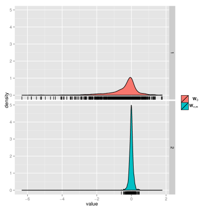
(a)

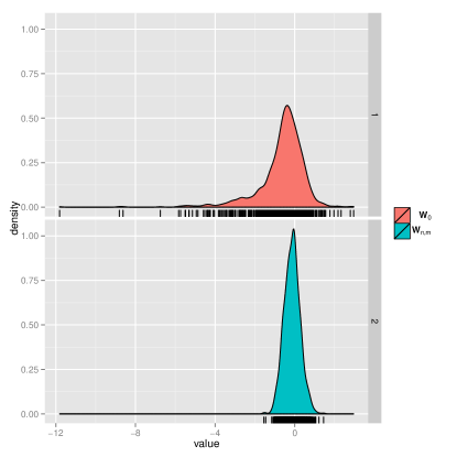
(b)

Figure 1: Comparison between the random $\mathbf{W}_{n,m}$ and fixed but unknown $\mathbf{W}_{0}$. The empirical distributions of $(m+n)(U_{n,m}(\hat{\mathbf{X}},\hat{\mathbf{Y}})-U_{n,m}(\mathbf{X},\mathbf{Y}\mathbf{W}_{0}))$ (in red) and $(m+n)(U_{n,m}(\hat{\mathbf{X}},\hat{\mathbf{Y}})-U_{n,m}(\mathbf{X},\mathbf{Y}\mathbf{W}_{n,m})$ (in blue) under (a) the null setting of $(\mathbf{X},\mathbf{A})\sim F,(\mathbf{Y},\mathbf{B})\sim F$ and (b) the alternative setting of $(\mathbf{X},\mathbf{A})\sim F,(\mathbf{Y},\mathbf{B})\sim G$.

We note that a subtle point in the statement and argument of the theorem is that $\mathbf{W}_{n,m}$ is a random quantity depending on $\mathbf{X}_{n}$ and $\mathbf{Y}_{m}$. There does exist a deterministic matrix $\mathbf{W}_{0}$ depending only on $F$ and $G$ such that $\mathbf{W}_{n,m}\rightarrow\mathbf{W}_{0}$ almost surely as $m,n\rightarrow\infty$. Indeed, from the proof of the theorem, we have that $\mathbf{W}_{1}$ is a $\sqrt{n}$-consistent estimator of $\mathbf{T}_{1}$ where $\mathbf{T}_{1}$ is the orthogonal matrix in the eigendecomposition of $\mathbb{E}[X_{1}X_{1}^{\top}]$ and that $\mathbf{W}_{2}$ is a $\sqrt{m}$-consistent estimator of $\mathbf{T}_{2}$ where $\mathbf{T}_{2}$ is the orthogonal matrix in the eigendecomposition of $\mathbb{E}[Y_{1}Y_{1}^{\top}]$. Under the null hypothesis, $F\circ\mathbf{T}_{1}=G\circ\mathbf{T}_{2}$; hence if we define $\mathbf{W}_{0}$ as $\mathbf{T}_{2}\mathbf{T}_{1}^{\top}$, then $\mathbf{W}_{2}\mathbf{W}_{1}^{\top}$ is a $\sqrt{n}$-consistent estimator of $\mathbf{W}_{0}$. This convergence of order $O(n^{-1/2})$ is, however, not sufficiently fast to guarantee that $(m+n)(U_{n,m}(\hat{\mathbf{X}},\hat{\mathbf{Y}})-U_{n,m}(\mathbf{X},\mathbf{Y}\mathbf{W}_{0}))$ converges to zero almost surely when $F\upVdash G$. For example, let $F$ be a mixture of two multivariate logit-normal distributions with mean parameters $(0,0),(4,4)$, identity covariance matrices and mixture components $(0.4,0.6)$; let $G$ be a multivariate logit-normal distribution with mean parameter $(2,2)$ and identity covariance matrix. Figure 1 illustrates that the difference $(m+n)(U_{n,m}(\hat{\mathbf{X}},\hat{\mathbf{Y}})-U_{n,m}(\mathbf{X},\mathbf{Y}\mathbf{W}_{n,m}))$ is in general smaller compared to the difference $(m+n)(U_{n,m}(\hat{\mathbf{X}},\hat{\mathbf{Y}})-U_{n,m}(\mathbf{X},\mathbf{Y}\mathbf{W}_{0}))$, thereby complicating the derivation of the exact nondegenerate limiting distribution for $(m+n)U_{m,n}(\hat{{\bf X}},\hat{{\bf Y}})$. Nevertheless, since the nondegenerate limiting distribution for $(m+n)U_{m,n}(\hat{{\bf X}},\hat{{\bf Y}})$ will not be distribution-free, the fact that it is currently unknown is, for all practical purposes, irrelevant. Indeed, the proposed test statistic still yields a consistent test procedure whose critical values can be obtained through a simple bootstrapping procedure.

Remark.

The computational cost for implementing the test procedure in Theorem 5 consist mainly of two parts, namely computing the adjacency spectral embedding of the graphs $\mathbf{A}$ and $\mathbf{B}$, and computing the test statistic $U_{n,m}(\hat{\mathbf{X}},\hat{\mathbf{Y}})$. Assuming $n\geq m$, the adjacency spectral embedding of $\mathbf{A}$ and $\mathbf{B}$ into $\mathbb{R}^{d}$ is a (partial) singular value decomposition of $\mathbf{A}$ and $\mathbf{B}$ and thus can be computed in $O(n^{2}d)$ time. The test statistic $U_{n,m}(\hat{\mathbf{X}},\hat{\mathbf{Y}})$ can be evaluated in $O(n^{2})$ time.

Remark.

The proof of Theorem 5 can be adapted to show that data-adaptive bandwidth selections behave similarly for $\hat{\mathbf{X}}$ and $\hat{\mathbf{Y}}$ as for $\mathbf{X}$ and $\mathbf{Y}$. That is to say, we can show that under the null hypothesis, $\Delta_{\theta}=(m+n)(U_{n,m}(\hat{\mathbf{X}},\hat{\mathbf{Y}})-U_{n,m}(\mathbf{X},\mathbf{Y}\mathbf{W}_{n,m}))$ converges to $0$ uniformly over some family of kernels $\{\kappa_{\theta}\colon\theta\in\Theta\}$. For example, $\{\kappa_{\theta}\colon\theta\in\Theta\}$ could be the set of Gaussian kernels with bandwidth $\theta\in\Theta$ for some bounded set $\Theta\subset\mathbb{R}_{+}$.

4 Experimental Results

In this section we illustrate our test statistic and procedure with two examples. The first example investigates the comparison of distinct two-block stochastic blockmodels. The second example considers graphs from a protein network dataset and uses our proposed test statistic to build a classifier.

4.1 Stochastic Blockmodel Example

We illustrate the hypothesis tests through several simulated and real data examples. For our first example, let $F_{\epsilon}$ for a given $\epsilon>0$ be mixture of point masses corresponding to a two-block stochastic block model with block membership probabilities $(0.4,0.6)$ and block probabilities $\mathbf{B}_{\epsilon}=\Bigl{[}\begin{smallmatrix}0.5+\epsilon&0.2\\ 0.2&0.5+\epsilon\end{smallmatrix}\Bigr{]}$. We then test, for a given $\epsilon>0$, the hypothesis $H_{0}\colon F_{0}\upVdash F_{\epsilon}$ against the alternative $H_{A}\colon F_{0}\nupVdash F_{\epsilon}$ using the kernel-based testing procedure of § 3. The kernel is chosen to be the Gaussian kernel with bandwidth $\sigma=0.5$. We first evaluate the performance through simulation using $1000$ Monte Carlo replicates; in each replicate we sample two graphs on $n$ vertices from $\mathrm{RDPG}(F_{0})$ and one graph on $n$ vertices from $\mathrm{RPDG}(F_{\epsilon})$. We then perform an adjacency spectral embedding on the graphs, in which we embed the graphs into $\mathbb{R}^{2}$, and we proceed to compute the kernel-based test statistic. We evaluate the performance of the test procedures for both $U_{n,m}(\mathbf{X},\mathbf{Y})$ and $U_{n,m}(\hat{\mathbf{X}},\hat{\mathbf{Y}})$ by estimating the power of the test statistic for various choices of $n\in\{100,200,500,1000\}$ and $\epsilon\in\{0.02,0.05,0.1\}$ through Monte Carlo simulation. The significance level is set to $\alpha=0.05$ and the rejection regions are specified via $B=200$ bootstrap permutation using either the true latent positions $\mathbf{X}$ and $\mathbf{Y}$ or the estimated latent positions $\hat{\mathbf{X}}$ and $\hat{\mathbf{Y}}$. These estimates are given in Table 1.

	$\epsilon=0.02$		$\epsilon=0.05$		$\epsilon=0.1$
$n$	$\{\mathbf{X},\mathbf{Y}\}$	$\{\hat{\mathbf{X}},\hat{\mathbf{Y}}\}$	$\{\mathbf{X},\mathbf{Y}\}$	$\{\hat{\mathbf{X}},\hat{\mathbf{Y}}\}$	$\{\mathbf{X},\mathbf{Y}\}$	$\{\hat{\mathbf{X}},\hat{\mathbf{Y}}\}$
$100$	$0.07$	$0.06$	$0.07$	$0.09$	$0.21$	$0.27$
$200$	$0.06$	$0.09$	$0.11$	$0.17$	$0.89$	$0.83$
$500$	$0.08$	$0.1$	$0.37$	$0.43$	$1$	$1$
$1000$	$0.1$	$0.14$	$1$	$1$	$1$	$1$

Table 1: Power estimates for testing the null hypothesis $F\upVdash G$ at a significance level of $\alpha=0.05$ using bootstrap permutation tests for the $U$-statistics $U_{n,m}(\hat{\mathbf{X}},\hat{\mathbf{Y}})$ and $U_{n,m}(\mathbf{X},\mathbf{Y})$. In each bootstrap test, $B=200$ bootstrap samples were generated. Each estimate of power is based on $1000$ Monte Carlo replicates of the corresponding bootstrap test.

4.2 Classification of protein networks

For our last example, we show how the statistics $U_{n,m}(\hat{\mathbf{X}},\hat{\mathbf{Y}})$ can also be adapted for use in graphs classification. More concretely, we consider the problem of classifying proteins network into enzyme versus non-enzymes. We use the dataset of Dobson and Doig [2003], which consists of $1178$ protein networks labeled as enzymes ($691$ networks) and non-enzymes ($487$ networks). For our classification procedure, we first embed each of the protein networks into $\mathbb{R}^{5}$ using adjacency spectral embedding. The choice of $d=5$ is chosen from among the choices of embedding dimensions ranging from $d=2$ through $d=15$ to minimize the classification error rate. We then compute a $1178\times 1178$ matrix $\mathbf{S}$ of pairwise dissimilarity between the adjacency spectral embedding of the protein networks using a Gaussian kernel with bandwidth $h=1$. The classifier is a $k$-NN classifier using the dissimilarities in $\mathbf{S}$ in place of the Euclidean distance. We evaluate the classification accuracy using a $10$-fold cross validation. The results are presented in Table 2. For the purpose of comparison, we also include the accuracy of several other classifiers that were previously applied on this data set, see Dobson and Doig [2003], Borgwardt et al. [2005]. The results of Dobson and Doig [2003] are based on modeling the proteins using various features such as secondary-structure content, surface properties, ligands, and amino acid propensities, and then training a SVM using a radial basis kernel on these feature vectors. The results of Borgwardt et al. [2005] are based on representing the proteins as graphs, using their secondary-structure content, and then training a SVM classifier using a random walk kernel on the result graphs. The accuracy of our straightforward classifier, which does not use any information about associated secondary structure, is comparable to that obtained from using SVM with a well-designed features kernel or well-designed graph kernels.

Classifier	Accuracy ($\%$)
SVM with optimized feature vector kernel [Dobson and Doig, 2003]	80.17
SVM with random walk kernel with secondary structure [Borgwardt et al., 2005]	77.30
$k$-NN with dissimilarities based on $U_{n,m}$	78.20

Table 2: Classification accuracy on the enzyme dataset.

5 Extensions

In this section we will consider extensions to alternative hypothesis tests that consider looser notions of equality between the two distributions. These notions may be quite useful in practice due to variations in graph properties that one may want to ignore in a comparison of the graphs. We do not formally state results for these extensions but we note that they can be derived in a similar manner to Theorem 5; see § A.1 and § A.2 in the appendix.

5.1 Scaling case

We now consider the case of testing the hypothesis that the distributions $F$ and $G$ are equal up to scaling. In particular the test

$$\quad H_{0}\colon F\upVdash G\circ c\quad\text{for some $c>0$}\quad\text{against}\quad H_{A}\colon F\nupVdash G\circ c\quad\text{for any $c>0$},$$

where $Y\sim F\circ c$ if $cY\sim F$. The test statistic is now a simple modification of the one in Theorem 5, i.e., we first scale the adjacency spectral embeddings by the norm of the empirical means before computing the kernel test statistic. In particular if we let

$$\hat{s}_{X}=n^{-1/2}\|\hat{\mathbf{X}}\|_{F},\quad\hat{s}_{Y}=m^{-1/2}\|\hat{\mathbf{Y}}\|_{F},\quad s_{X}=n^{-1/2}\|\mathbf{X}\|_{F},\quad s_{Y}=m^{-1/2}\|\mathbf{Y}\|_{F},$$

then the conclusions of Theorem 5 hold where we use $U_{n,m}(\hat{\mathbf{X}}/\hat{s}_{X},\hat{\mathbf{Y}}/\hat{s}_{Y})$ as the test statistic in comparison to $U_{n,m}(\mathbf{X}/s_{X},\mathbf{Y}\mathbf{W}_{n,m}/s_{Y})$. Note that we must restrict $c$ so that $G\circ c$ is still a valid distribution for an RDPG.

As an example let $F_{\epsilon}$ be the uniform distribution on $[\epsilon,1/\sqrt{2}]^{2}$ where $\epsilon\geq 0$ and let $G$ be the uniform distribution on $[0,1/\sqrt{3}]^{2}$. For a given $\epsilon$, we test the hypothesis $H_{0}\colon F_{\epsilon}\upVdash G\circ c$ for some constant $c>0$ against the alternative $H_{A}\colon F_{\epsilon}\nupVdash G\circ c$ for any constant $c>0$. The testing procedure is based on the test statistic $(m+n)U_{n,m}(\hat{\mathbf{X}}/\hat{s}_{X},\hat{\mathbf{Y}}/\hat{s}_{Y})$ using a Gaussian kernel with bandwidth $\sigma=0.5$. Table 3 is the analogue of Table 1 and presents estimates of the size and power for $U_{n,m}(\mathbf{X}/s_{X},\mathbf{Y}/s_{Y})$ and $U_{n,m}(\hat{\mathbf{X}}/\hat{s}_{X},\hat{\mathbf{Y}}/\hat{s}_{Y})$ for various choices of $n$ and $\epsilon$.

	$\epsilon=0$		$\epsilon=0.05$		$\epsilon=0.1$		$\epsilon=0.2$
$n$	$\{\mathbf{X},\mathbf{Y}\}$	$\{\hat{\mathbf{X}},\hat{\mathbf{Y}}\}$	$\{\mathbf{X},\mathbf{Y}\}$	$\{\hat{\mathbf{X}},\hat{\mathbf{Y}}\}$	$\{\mathbf{X},\mathbf{Y}\}$	$\{\hat{\mathbf{X}},\hat{\mathbf{Y}}\}$	$\{\mathbf{X},\mathbf{Y}\}$	$\{\hat{\mathbf{X}},\hat{\mathbf{Y}}\}$
$100$	$0.05$	$0.04$	$0.184$	$0.02$	$0.79$	$0.16$	1	0.91
$200$	$0.06$	$0.1$	$0.39$	$0.11$	$0.98$	$0.7$	1	1
$500$	$0.07$	$0.07$	$0.83$	$0.66$	$1$	$1$	1	1
$1000$	$0.06$	$0.03$	$1$	$0.98$	$1$	$1$	1	1

Table 3: Power estimates for testing the null hypothesis $F\upVdash G\circ c$ at a significance level of $\alpha=0.05$ using bootstrap permutation tests for the $U$-statistics $U_{n,m}(\hat{\mathbf{X}}/\hat{s}_{X},\hat{\mathbf{Y}}/\hat{s}_{Y})$ and $U_{n,m}(\mathbf{X}/s_{X},\mathbf{Y}/s_{Y})$. In each bootstrap test, $B=200$ bootstrap samples were generated. Each estimate of power is based on $1000$ Monte Carlo replicates of the corresponding bootstrap test. The entries for $\epsilon=0$ coincides with bootstrap estimate for the size of the test.

5.2 Projection case

We next consider the case of testing

$$\quad H_{0}\colon F\circ\pi^{-1}\upVdash G\circ\pi^{-1}\quad\text{against}\quad H_{A}\colon F\circ\pi^{-1}\nupVdash G\circ\pi^{-1},$$

where $\pi$ is the projection $x\mapsto x/\|x\|$ that maps $x$ onto the unit sphere in $\mathbb{R}^{d}$. In an abuse of notation we will also write $\pi(\mathbf{X})$ to denote the row-wise projection of the rows of $\mathbf{X}$ onto the unit sphere.

We shall assume that $0$ is not an atom of either $F$ or $G$, i.e., $F(0)=G(0)=0$, for otherwise the problem is possibly ill-posed: specifically, $\pi(0)$ is undefined. In addition, for simplicity in the proof, we shall also assume that the support of $F$ and $G$ is bounded away from $0$, i.e., there exists some $\epsilon>0$ such that $F(\{x\colon\|x\|\leq\epsilon\})=G(\{x\colon\|x\|\leq\epsilon\})=0$. A truncation argument with $\epsilon\rightarrow 0$ allows us to handle the general case of distributions on $\Omega$ where $0$ is not an atom.

To contextualize the test of equality up to projection, consider the very specific case of the degree-corrected stochastic blockmodel [Karrer and Newman, 2011]. A degree-corrected stochastic blockmodel can be view as a random dot product graph whose latent position $X_{v}$ for an arbitrary vertex $v$ is of the form $X_{v}=\theta_{v}\nu_{v}$ where $\nu_{v}$ is sampled from a mixture of point masses and $\theta_{v}$ (the degree-correction factor) is sampled from a distribution on $(0,1]$. Thus, given two degree-corrected stochastic blockmodel graphs, equality up to projection tests whether the underlying mixture of point masses (that is, the distribution of the $\nu_{v}$) are the same modulo the distribution of the degree-correction factors $\theta_{v}$.

For this test, under the assumption that both $F$ and $G$ have supports bounded away from the origin, the conclusions of Theorem 5 hold where we use $U_{n,m}(\pi(\hat{\mathbf{X}}),\pi(\hat{\mathbf{Y}}))$ as the test statistic and compare it to $U_{n,m}(\pi(\mathbf{X}),\pi(\mathbf{Y})\mathbf{W}_{n,m})$.

5.3 Local alternatives and sparsity

We now consider the test procedure of Theorem 5 in the context of (1) local alternatives and (2) sparsity. It is not hard to show that the test statistic $U_{n,m}(\hat{\mathbf{X}},\hat{\mathbf{Y}})$ is also consistent against local alternatives, in particular the setting $(\mathbf{X}_{n},\mathbf{A}_{n})\sim\mathrm{RDPG}(F_{n})$, $(\mathbf{Y}_{n},\mathbf{B}_{n})\sim\mathrm{RDPG}(G_{n})$ with $\|\mu[F_{n}]-\mu[G_{n}]\|_{\mathcal{H}}\rightarrow 0$. In this setting, the accuracy of $\hat{\mathbf{X}}_{n}$ and $\hat{\mathbf{Y}}_{n}$ as estimates for $\mathbf{X}_{n}$ and $\mathbf{Y}_{n}$ is unchanged; the only difference is that the distance between $F_{n}$ and $G_{n}$ is shrinking. Thus Eq. (3.5) and Eq. (3.6) continue to hold and the test procedure is consistent against all local alternatives for which $\|\mu[F]-\mu[G]\|_{\mathcal{H}}=\omega(n^{-1/2}\log^{K}(n))$ for some integer $K\geq 2$ (c.f. Gretton et al. [2012, Theorem 13]).

Another related setting is that of sparsity, in which $(\mathbf{X}_{n},\mathbf{A}_{n})\sim\mathrm{RDPG}(\alpha_{n}^{1/2}F)$, $(\mathbf{Y}_{n},\mathbf{B}_{n})\sim\mathrm{RDPG}(\alpha_{n}^{1/2}G)$, with $F$ and $G$ being fixed distributions but the sparsity factor $\alpha_{n}\rightarrow 0$. That is to say, $(\mathbf{X}_{n},\mathbf{A}_{n})\sim\mathrm{RDPG}(\alpha_{n}^{1/2}F)$ for $\alpha_{n}\leq 1$ if the rows of $\mathbf{X}_{n}$ are sampled i.i.d from $F$ and, conditioned on $\mathbf{X}_{n}$, $\mathbf{A}_{n}$ is a random $n\times n$ adjacency matrix with probability

$$\mathbb{P}[\mathbf{A}|\{X_{i}\}_{i=1}^{n}]=\prod_{i\leq j}(\alpha_{n}X_{i}^{\top}X_{j})^{\mathbf{A}_{ij}}(1-\alpha_{n}X_{i}^{\top}X_{j})^{1-\mathbf{A}_{ij}}.$$

Now the accuracy of $\hat{\mathbf{X}}_{n}$ and $\hat{\mathbf{Y}}_{n}$ as estimates for $\mathbf{X}_{n}$ and $\mathbf{Y}_{n}$ decreases with $\alpha_{n}$ due to increasing sparsity. More specifically, if $\hat{\mathbf{X}}_{n}$ denotes the adjacency spectral embedding of $\mathbf{A}_{n}$ where $(\mathbf{X}_{n},\mathbf{A}_{n})\sim\mathrm{RDPG}(\alpha_{n}F)$, then Lemma 2 can be extended to yield that, with probability at least $1-4\eta$, there exists an orthogonal matrix $\mathbf{W}_{n}$ such that

$$\|\alpha_{n}^{-1/2}\hat{\mathbf{X}}_{n}-\mathbf{X}_{n}\mathbf{W}_{n}\|_{F}\leq\alpha_{n}^{-1/2}C_{1}$$ (5.1)

for some constant $C_{1}$. We note that there are $n$ rows in $\hat{\mathbf{X}}_{n}$ and hence, on average, we have that for each index $i$, $\|\alpha_{n}^{-1/2}\hat{X}_{i}-\mathbf{W}_{n}X_{i}\|\leq(n\alpha_{n})^{-1/2}C_{1}$ with high probability. Thus, if $n\alpha_{n}\rightarrow\infty$, we have that, on average, each $\alpha_{n}^{-1/2}\hat{X}_{i}$ is a consistent estimate of the corresponding $X_{i}$. Thus we should expect that there exists some sequence of orthogonal matrices $\mathbf{V}_{n}$ such that $|U_{n,m}(\alpha_{n}^{-1/2}\hat{\mathbf{X}}_{n},\alpha_{n}^{-1/2}\hat{\mathbf{Y}}_{n})-U_{n,m}(\mathbf{X}_{n},\mathbf{Y}_{n}\mathbf{V}_{n})|\rightarrow 0$ as $n\rightarrow\infty$. More formally, we have the following.

Proposition 6.

Let $(\mathbf{X}_{n},\mathbf{A}_{n})\sim\mathrm{RDPG}(\alpha_{n}^{1/2}F)$ and $(\mathbf{Y}_{m},\mathbf{B}_{m})\sim\mathrm{RDPG}(\beta_{m}^{1/2}G)$ be independent random dot product graphs with latent position distributions $F$ and $G$ and sparsity factor $\alpha_{n}$ and $\beta_{m}$, respectively. Furthermore, suppose that both $F$ and $G$ satisfies the distinct eigenvalues condition in Assumption 1 and that $\alpha_{n}$ and $\beta_{m}$ are known. Consider the hypothesis test

$$H_{0}\colon F\upVdash G\quad\text{against}\quad H_{A}\colon F\nupVdash G.$$

Denote by $\hat{\mathbf{X}}_{n}=\{\hat{X}_{1},\dots,\hat{X}_{n}\}$ and $\hat{\mathbf{Y}}_{m}=\{\hat{Y}_{1},\dots,\hat{Y}_{m}\}$ the adjacency spectral embedding of $\mathbf{A}_{n}$ and $\mathbf{B}_{m}$, respectively. Let $\mathbf{W}_{1}$ and $\mathbf{W}_{2}$ be $d\times d$ orthogonal matrices in the eigendecomposition $\mathbf{W}_{1}\mathbf{S}_{1}\mathbf{W}_{1}^{\top}=\mathbf{X}_{n}^{\top}\mathbf{X}_{n}$, $\mathbf{W}_{2}\mathbf{S}_{2}\mathbf{W}_{2}=\mathbf{Y}_{m}^{\top}\mathbf{Y}_{m}$, respectively. Suppose that $m,n\rightarrow\infty$, $\tfrac{m}{m+n}\rightarrow\rho\in(0,1)$ and furthermore that $n\alpha_{n}=\omega(\log^{4}{n})$ and $m\beta_{m}=\omega(\log^{4}m)$. Then the sequence of matrices $\mathbf{W}_{n,m}=\mathbf{W}_{2}\mathbf{W}_{1}^{\top}$ satisfies

$$U_{n,m}(\alpha_{n}^{-1/2}\hat{\mathbf{X}}_{n},\beta_{m}^{-1/2}\hat{\mathbf{Y}}_{m})-U_{n,m}(\mathbf{X}_{n},\mathbf{Y}_{m}\mathbf{W}_{n,m})\overset{\mathrm{a.s.}}{\longrightarrow}0.$$ (5.2)

Proof Sketch.

Let $\psi=U_{n,m}(\alpha_{n}^{-1/2}\hat{\mathbf{X}}_{n},\beta_{m}^{-1/2}\hat{\mathbf{Y}}_{m})-U_{n,m}(\mathbf{X}_{n},\mathbf{Y}_{m}\mathbf{W}_{n,m})$. We have

$$\begin{split}\psi&=\frac{1}{n(n-1)}\sum_{j\not=i}(\kappa(\alpha_{n}^{-1/2}\hat{X}_{i},\alpha_{n}^{-1/2}\hat{X}_{j})-\kappa(\mathbf{W}_{1}X_{i},\mathbf{W}_{1}X_{j}))\\ &-\frac{2}{mn}\sum_{i=1}^{n}\sum_{k=1}^{m}(\kappa(\alpha_{n}^{-1/2}\hat{X}_{i},\beta_{m}^{-1/2}\hat{Y}_{k})-\kappa(\mathbf{W}_{1}X_{i},\mathbf{W}_{2}Y_{k}))\\ &+\frac{1}{m(m-1)}\sum_{l\not=k}\kappa(\beta_{m}^{-1/2}\hat{Y}_{k},\beta_{m}^{-1/2}\hat{Y}_{l})-\kappa(\mathbf{W}_{2}Y_{k},\mathbf{W}_{2}Y_{l})).\end{split}$$

Let $\mathcal{S}_{X}\subset\{1,2,\dots,n\}$ and $\mathcal{S}_{Y}\subset\{1,2,\dots,m\}$ be defined by

$$\mathcal{S}_{X}=\{i\,\,\colon\,\,\|\alpha_{n}^{-1/2}\hat{X}_{i}-\mathbf{W}_{1}X_{i}\|\leq C_{1}(n\alpha_{n})^{-1/2}\log{n}\},$$

$$\mathcal{S}_{Y}=\{k\,\,\colon\,\,\|\beta_{m}^{-1/2}\hat{Y}_{k}-\mathbf{W}_{2}Y_{k}\|\leq C_{2}(m\beta_{m})^{-1/2}\log{m}\}.$$

From Eq. (5.1), the number of indices $i\not\in S_{X}$ is of order $o(n)$, with high probability. Similarly, the number of indices $k\not\in S_{Y}$ is of order $o(m)$ with high probability. Therefore,

$$\begin{split}\psi&=\frac{1}{n(n-1)}\sum_{i\in S_{X}}\sum_{j\in S_{X}}(\kappa(\alpha_{n}^{-1/2}\hat{X}_{i},\alpha_{n}^{-1/2}\hat{X}_{j})-\kappa(\mathbf{W}_{1}X_{i},\mathbf{W}_{1}X_{j}))\\ &-\frac{2}{mn}\sum_{i\in S_{X}}\sum_{k\in S_{Y}}(\kappa(\alpha_{n}^{-1/2}\hat{X}_{i},\beta_{m}^{-1/2}\hat{Y}_{k})-\kappa(\mathbf{W}_{1}X_{i},\mathbf{W}_{2}Y_{k}))\\ &+\frac{1}{m(m-1)}\sum_{k\in S_{Y}}\sum_{l\in S_{Y}}\kappa(\beta_{m}^{-1/2}\hat{Y}_{k},\beta_{m}^{-1/2}\hat{Y}_{l})-\kappa(\mathbf{W}_{2}Y_{k},\mathbf{W}_{2}Y_{l}))+o(1).\end{split}$$

We consider the term $1/(n(n-1))\sum_{i\in S_{X}}\sum_{j\in S_{X}}(\kappa(\alpha_{n}^{-1/2}\hat{X}_{i},\alpha_{n}^{-1/2}\hat{X}_{j})-\kappa(\mathbf{W}_{1}X_{i},\mathbf{W}_{1}X_{j}))$. By the differentiability of $\kappa$ and compactness of $\Omega$, we have

$$|\kappa(\alpha_{n}^{-1/2}\hat{X}_{i},\alpha_{n}^{-1/2}\hat{X}_{j})-\kappa(\mathbf{W}_{1}X_{i},\mathbf{W}_{1}X_{j})|\leq C\max\{\|\alpha_{n}^{-1/2}\hat{X}_{i}-\mathbf{W}_{1}X_{i}\|,\|\alpha_{n}^{-1/2}\hat{X}_{j}-\mathbf{W}_{1}X_{j}\|\}$$

for some constant $C$ independent of $i$ and $j$. Thus,

$$\Bigl{|}\frac{1}{n(n-1)}\sum_{i\in S_{X}}\sum_{j\in S_{X}}(\kappa(\alpha_{n}^{-1/2}\hat{X}_{i},\alpha_{n}^{-1/2}\hat{X}_{j})-\kappa(\mathbf{W}_{1}X_{i},\mathbf{W}_{n}X_{j}))\Bigr{|}\leq\max_{i\in S_{X}}C\|\alpha_{n}^{-1/2}\hat{X}_{i}-\mathbf{W}_{1}X_{i}\|.$$

Similar reasoning yields

$$\begin{split}|\psi|&\leq 2C(\max_{i\in S_{X}}\|\alpha_{n}^{-1/2}\hat{X}_{i}-\mathbf{W}_{1}X_{i}\|+\max_{k\in S_{Y}}\|\beta_{m}^{-1/2}\hat{Y}_{k}-\mathbf{W}_{2}Y_{k}\|)+o(1)\\ &\leq 2C(C_{1}(n\alpha_{n})^{-1/2}\log n+C_{2}(m\beta_{m})^{-1/2}\log m)+o(1)\end{split}$$

with high probability. As $n\alpha_{n}=\omega(\log^{4}n)$ and $m\beta_{m}=\omega(\log^{4}m)$, we have $\psi\overset{\mathrm{a.s.}}{\longrightarrow}0$ as $m,n\rightarrow\infty$. ∎

We assume in the statement of Proposition 6 that the sparsity factors $\alpha_{n}$ and $\beta_{m}$ are known. If $\alpha_{n}$ and $\beta_{m}$ are unknown, then they can be estimated from the adjacency spectral embedding of $\mathbf{A}_{n}$ and $\mathbf{B}_{m}$, but only up to some constant factor. Hence the hypothesis test of

$$H_{0}\colon F\upVdash G\quad\text{against}\quad H_{A}\colon F\nupVdash G$$

is no longer meaningful (as the sparsity factors $\alpha_{n}$ and $\beta_{m}$ cannot be determined uniquely) and one should consider instead the hypothesis test of equality up to scaling of § 5.1.

We note that the conclusion of Proposition 6, namely Eq. (5.2), is weaker than that of Theorem 5 due to the lack of the $m+n$ factor in Eq. (5.2) as compared to Eq. (3.5) and Eq. (3.6). The more difficult question, and one which we will not address in this paper, is to refine the rate of convergence to zero of Eq. (5.2) in the sparse setting. We suspect, however, that Eq. (3.5) will not hold in the case where $\alpha_{n}=o(n^{-1/2})$ and $\beta_{m}=o(m^{-1/2})$. Nevertheless, Proposition 6 still yields yields a test procedure that is consistent against any alternative, provided that both $F$ and $G$ satisfy Assumption 1, and that the sparsity factors $\alpha_{n}$ and $\beta_{m}$ do not converge to $0$ too quickly.

6 Discussion

In summary, we show in this paper that the adjacency spectral embedding can be used to generate simple and intuitive test statistics for the nonparametric inference problem of testing whether two random dot product graphs have the same or related distribution of latent positions. The two-sample formulations presented here and the corresponding test statistics are intimately related. Indeed, for random dot product graphs, the adjacency spectral embedding yields a consistent estimate of the latent positions as points in $\mathbb{R}^{d}$; there then exist a wide variety of classical and well-studied testing procedures for data in Euclidean spaces.

New results on stochastic blockmodels suggest that they can be regarded as a universal approximation to graphons in exchangeable random graphs, see e.g., Yang et al. [2014], Wolfe and Olhede [2013]. There is thus potential theoretical value in the formulation of two-sample hypothesis testing for latent position models in terms of a random dot product graph model on $\mathbb{R}^{d}$ with possibly varying $d$. However, because the link function and the distribution of latent positions are intertwined in the context of latent position graphs, any proposed test procedure that is sufficiently general might also possess little to no power.

The two-sample hypothesis testing we consider here is also closely related to the problem of testing goodness-of-fit; the results in this paper can be easily adapted to address the latter question. In particular, we can test, for a given graph, whether the graph is generated from some specified stochastic blockmodel. A more general problem is that of testing whether a given graph is generated according to a latent position model with a specific link function. This problem has been recently studied; see Yang et al. [2014] for a brief discussion, but much remains to be investigated. For example, the limiting distribution of the test statistic in Yang et al. [2014] is not known.

Finally, two-sample hypothesis testing is also closely related to testing for independence; given a random sample $\{(X_{i},Y_{i})\}$ with joint distribution $F_{XY}$ and marginal distributions $F_{X}$ and $F_{Y}$, $X$ and $Y$ are independent if the $F_{XY}$ differs from the product $F_{X}F_{Y}$. For example, the Hilbert-Schmidt independence criterion is a measure for statistical dependence in terms of the Hilbert-Schmidt norm of a cross-covariance operator. It is based on the maximum mean discrepancy between $F_{XY}$ and $F_{X}F_{Y}$. Another example is Brownian distance covariance of Székely and Rizzo [2009], a measure of dependence based on the energy distance between $F_{XY}$ and $F_{X}F_{Y}$. In particular, consider the test of whether two given two random dot product graphs $(\mathbf{X},\mathbf{A})\sim\mathrm{RDPG}(F_{X})$ and $(\mathbf{Y},\mathbf{B})\sim\mathrm{RDPG}(F_{Y})$ on the same vertex set have independent latent position distributions $F_{X}$ and $F_{Y}$. While we surmise that it may be possible to adapt our present results to this question, we stress that the conditional independence of $\mathbf{A}$ given $\mathbf{X}$ and of $\mathbf{B}$ given $\mathbf{Y}$ suggests that independence testing may merit a more intricate approach.

Appendix A Additional Proofs

Proof of Lemma 3: As $\kappa$ is twice continuously differentiable, $\mathcal{F}$ is also twice continuously differentiable [Steinwart and Christmann, 2008, Corollary 4.36]. Denote by $\mathbf{W}$ the orthogonal matrix such that $\mathbf{X}=\mathbf{U}_{\mathbf{P}}\mathbf{S}_{\mathbf{P}}^{1/2}\mathbf{W}$.

Let $f\in\mathcal{F}_{\Phi}$, a Taylor expansion of $f$ then yields

$$\begin{split}\frac{1}{\sqrt{n}}\sum_{i=1}^{n}\Bigl{(}f(\mathbf{W}\hat{X}_{i})-f(X_{i})\Bigr{)}&=\frac{1}{\sqrt{n}}\sum_{i=1}^{n}(\partial f)(X_{i})^{\top}(\mathbf{W}\hat{X}_{i}-X_{i})\\ &+\frac{1}{2\sqrt{n}}\sum_{i}(\mathbf{W}\hat{X}_{i}-X_{i})^{\top}(\partial^{2}f)(X_{i}^{*})(\mathbf{W}\hat{X}_{i}-X_{i})\end{split}$$

where, for any $i$, $X_{i}^{*}\in\mathbb{R}^{d}$ is such that $\|X_{i}^{*}-X_{i}\|\leq\|\mathbf{W}\hat{X}_{i}-X_{i}\|$. We first bound the quadratic terms, i.e. those depending on $\partial^{2}f$. We note that since $\kappa$ is twice continuously differentiable, $\sup_{f\in\mathcal{F}_{\Phi},X\in\Omega}\|(\partial^{2}f)(X)\|$ is bounded (the norm under consideration is the spectral norm on matrices). Therefore,

$$\begin{split}\sup_{f\in\mathcal{F}_{\Phi}}\Big{|}\sum_{i=1}^{n}\frac{(\mathbf{W}\hat{X}_{i}-X_{i})^{\top}(\partial^{2}f)(X_{i}^{*})(\mathbf{W}\hat{X}_{i}-X_{i})}{\sqrt{n}}\Big{|}&\leq\sup_{f\in\mathcal{F},X\in\Omega}\frac{\|(\partial^{2}f)(X)\|\|\hat{\mathbf{X}}\mathbf{W}-\mathbf{X}\|_{F}^{2}}{\sqrt{n}}.\end{split}$$

Hence, by applying Lemma 2 to bound $\|\hat{\mathbf{X}}\mathbf{W}-\mathbf{X}\|_{F}^{2}$ in the above expression, we have

$$\sup_{f\in\mathcal{F}_{\Phi}}\Big{|}\sum_{i=1}^{n}\frac{(\mathbf{W}\hat{X}_{i}-X_{i})^{\top}(\partial^{2}f)(X_{i}^{*})(\mathbf{W}\hat{X}_{i}-X_{i})}{\sqrt{n}}\Big{|}\overset{\mathrm{a.s.}}{\longrightarrow}0$$

as $n\rightarrow\infty$.

We now bound the linear terms, i.e., those depending on $\partial f$. For any $f\in\mathcal{F}_{\Phi}$, and any $X_{1},\dots,X_{n}$, let $\mathbf{M}(\partial f)=\mathbf{M}(\partial f;X_{1},\cdots,X_{n})\in\mathbb{R}^{n\times d}$ be the matrix whose rows are the vectors $(\partial f)(X_{i})$. We then have

$$\begin{split}\zeta(f)&:=\frac{1}{\sqrt{n}}\sum_{i=1}^{n}(\partial f)(X_{i})^{\top}(\mathbf{W}\hat{X}_{i}-X_{i})\\ &=\frac{1}{\sqrt{n}}\mathrm{tr}\Bigl{(}(\hat{\mathbf{X}}\mathbf{W}-\mathbf{X})[\mathbf{M}(\partial f)]^{\top}\Bigr{)}=\frac{1}{\sqrt{n}}\mathrm{tr}\Bigl{(}(\mathbf{U}_{\mathbf{A}}\mathbf{S}_{\mathbf{A}}^{1/2}-\mathbf{U}_{\mathbf{P}}\mathbf{S}_{\mathbf{P}}^{1/2})\mathbf{W}[\mathbf{M}(\partial f)]^{\top}\Bigr{)}.\end{split}$$

Now $\mathbf{A}=\mathbf{U}_{\mathbf{A}}\mathbf{S}_{\mathbf{A}}\mathbf{U}_{\mathbf{A}}^{\top}+\mathbf{E}$ where, as we recall in Definition 2, $\mathbf{S}_{\mathbf{A}}$ is the diagonal matrix containing the $d$ largest eigenvalues of $|\mathbf{A}|$ (which coincides, with high probability, with the eigenvalues of $A$) and $\mathbf{U}_{\mathbf{A}}$ is the matrix whose columns are the corresponding eigenvectors. The eigendecomposition of $\mathbf{E}$ can be written in terms of the eigenvalues and eigenvectors that are not included in $\mathbf{S}_{\mathbf{A}}$ and $\mathbf{U}_{\mathbf{A}}$. Thus $\mathbf{E}\mathbf{U}_{\mathbf{A}}=\bm{0}$ and $\mathbf{U}_{\mathbf{A}}\mathbf{S}_{\mathbf{A}}^{1/2}=\mathbf{U}_{\mathbf{A}}\mathbf{S}_{\mathbf{A}}\mathbf{U}_{\mathbf{A}}^{\top}\mathbf{U}_{\mathbf{A}}\mathbf{S}_{\mathbf{A}}^{-1/2}=(\mathbf{U}_{\mathbf{A}}\mathbf{S}_{\mathbf{A}}\mathbf{U}_{\mathbf{A}}^{\top}+\mathbf{E})\mathbf{U}_{\mathbf{A}}\mathbf{S}_{\mathbf{A}}^{-1/2}=\mathbf{A}\mathbf{U}_{\mathbf{A}}\mathbf{S}_{\mathbf{A}}^{-1/2}$. Similarly, $\mathbf{P}=\mathbf{U}_{\mathbf{P}}\mathbf{S}_{\mathbf{P}}\mathbf{U}_{\mathbf{P}}^{\top}$ (because $\mathbf{P}$ is rank $d$) and $\mathbf{U}_{\mathbf{P}}\mathbf{S}_{\mathbf{P}}^{1/2}=\mathbf{P}\mathbf{U}_{\mathbf{P}}\mathbf{S}_{\mathbf{P}}^{-1/2}$. Thus,

$$\begin{split}\zeta(f)&=\frac{1}{\sqrt{n}}\mathrm{tr}\Bigl{(}\mathbf{A}\mathbf{U}_{\mathbf{A}}\mathbf{S}_{\mathbf{A}}^{-1/2}-\mathbf{P}\mathbf{U}_{\mathbf{P}}\mathbf{S}_{\mathbf{P}}^{-1/2}\Bigr{)}\mathbf{W}[\mathbf{M}(\partial f)]^{\top}\Bigr{)}\\ &=\frac{1}{\sqrt{n}}\mathrm{tr}\Bigl{(}\Bigl{(}\mathbf{A}(\mathbf{U}_{\mathbf{A}}-\mathbf{U}_{\mathbf{P}})\mathbf{S}_{\mathbf{A}}^{-1/2}+\mathbf{A}\mathbf{U}_{\mathbf{P}}(\mathbf{S}_{\mathbf{A}}^{-1/2}-\mathbf{S}_{\mathbf{P}}^{-1/2})+(\mathbf{A}-\mathbf{P})\mathbf{U}_{\mathbf{P}}\mathbf{S}_{\mathbf{P}}^{-1/2}\Bigr{)}\mathbf{W}[\mathbf{M}(\partial f)]^{\top}\Bigr{)}.\end{split}$$

We therefore have

$$\begin{split}\sup_{f\in\mathcal{F}_{\Phi}}|\zeta(f)|&\leq\frac{\sup_{f\in\mathcal{F}_{\Phi}}\|\mathbf{M}(\partial f)\|_{F}}{\sqrt{n}}\Bigl{(}\|\mathbf{A}(\mathbf{U}_{\mathbf{A}}-\mathbf{U}_{\mathbf{P}})\mathbf{S}_{\mathbf{A}}^{-1/2}\mathbf{W}\|_{F}+\|\mathbf{A}\mathbf{U}_{\mathbf{P}}(\mathbf{S}_{\mathbf{A}}^{-1/2}-\mathbf{S}_{\mathbf{P}}^{-1/2})\mathbf{W}\|_{F}\Bigr{)}\\ &+\frac{1}{\sqrt{n}}\,\,\sup_{f\in\mathcal{F}_{\Phi}}|\mathrm{tr}\Bigl{(}[\mathbf{M}(\partial f)]^{T}(\mathbf{A}-\mathbf{P})\mathbf{U}_{\mathbf{P}}\mathbf{S}_{\mathbf{P}}^{-1/2}\mathbf{W}\Bigr{)}|.\end{split}$$ (A.1)

We bound the first two terms on the right hand side of Eq. (A.1) using the following result from Lyzinski et al. [2014].

Lemma 7.

Let $(\mathbf{X},\mathbf{A})\sim\mathrm{RDPG}(F)$ and let $c>0$ be arbitrary but fixed. There exists $n_{0}(c)$ such that if $n>n_{0}$ and $\eta$ satisfies $n^{-c}<\eta<1/2$, then with probability at least $1-2\eta$, the following bounds hold simultaneously

$$\|\mathbf{A}(\mathbf{U}_{\mathbf{A}}-\mathbf{U}_{\mathbf{P}})\mathbf{S}_{\mathbf{A}}^{-1/2}\|_{F}\leq\frac{24\sqrt{2}d\log{(n/\eta)}}{\sqrt{\gamma^{5}(F)n}},$$ (A.2)

$$\|\mathbf{A}\mathbf{U}_{\mathbf{P}}(\mathbf{S}_{\mathbf{A}}^{-1/2}-\mathbf{S}_{\mathbf{P}}^{-1/2})\|_{F}\leq\frac{48d\log{(n/\eta)}}{\sqrt{\gamma^{7}(F)n}},$$ (A.3)

where $\gamma(F)$ is the minimum gap between the distinct eigenvalues of the matrix $\mathbb{E}[X_{1}X_{1}^{\top}]$ with $X_{1}\sim F$.

Eq. (A.2) in the above lemma is a restatement of Lemma 3.4 in Lyzinski et al. [2014] where we have used the fact that the maximum row sum of $\mathbf{A}$ is $n$. Eq. (A.3) follows from Lemma 3.2 in Lyzinski et al. [2014] and the fact that $\|\mathbf{M}_{1}\mathbf{M}_{2}\|_{2\to\infty}\leq\|\mathbf{M}_{1}\|_{2\to\infty}\|\mathbf{M}_{2}\|$ for any matrices $\mathbf{M}_{1}$ and $\mathbf{M}_{2}$. As the individual bound in Eq. (A.2) and Eq. (A.3) holds with probabilty $1-\eta$, they hold simultaneously with probability $1-2\eta$.

Lemma 7 then yields

$$\frac{\sup_{f\in\mathcal{F}_{\Phi}}\|\mathbf{M}(\partial f)\|_{F}}{\sqrt{n}}\Bigl{(}\|\mathbf{A}(\mathbf{U}_{\mathbf{A}}-\mathbf{U}_{\mathbf{P}})\mathbf{S}_{\mathbf{A}}^{-1/2}\mathbf{W}\|_{F}+\|\mathbf{A}\mathbf{U}_{\mathbf{P}}(\mathbf{S}_{\mathbf{A}}^{-1/2}-\mathbf{S}_{\mathbf{P}}^{-1/2})\mathbf{W}\|_{F}\Bigr{)}\leq\frac{C(F)\log{n}}{\sqrt{n}}$$

with probability at least $1-n^{-2}$, where $C(F)$ is a constant depending only on $F$.

We next show that the last term on the right hand side of Eq. (A.1) is also of order $n^{-1/2}(\log{n})$ with probability at least $1-n^{-2}$. To control this supremum, we use a chaining argument. Denote by $\partial\mathcal{F}_{\Phi}$ the space of functions $\partial\mathcal{F}_{\Phi}=\{\partial f\colon f\in\mathcal{F}_{\Phi}\}$ from $\mathbb{R}^{d}$ to $\mathbb{R}^{d}$. For a given $\partial f\in\partial\mathcal{F}_{\Phi}$ let $\|\partial f\|_{\infty}$ denote the quantity $\sup_{X\in\Omega}\|(\partial f)(X)\|_{2}$, where $\|\cdot\|_{2}$ is the Euclidean norm in $\mathbb{R}^{d}$. Similarly, for given $\partial f,\partial g\in\mathcal{\partial F}_{\Phi}$, let $\|\partial f-\partial g\|_{\infty}$ denote $\sup_{X\in\Omega}\|(\partial f-\partial g)(X)\|_{2}$. As $\kappa$ is twice continuously differentiable and $\Omega$ is compact, $\mathcal{\partial F}_{\Phi}$ is totally bounded with respect to $\|\cdot\|_{\infty}$. Put $\delta=\sup_{\partial f\in\mathcal{\partial F}_{\Phi}}\|\partial f\|_{\infty}$. Then for any $j\in\mathbb{N}$, we can find a finite subset $S_{j}=\{\partial f_{1},\partial f_{2},\dots,\partial f_{n_{j}}\}$ of $\partial\mathcal{F}_{\Phi}$ such that for any $\partial f\in\partial\mathcal{F}_{\Phi}$, there exists a $\partial f_{l}\in S_{j}$ with $\|\partial f-\partial f_{l}\|_{\infty}\leq\delta_{j}:=2^{-j}\delta$. We shall assume that $S_{j}$ is minimal among all sets with the above property.

Given $S_{j}$, define $\Pi_{j}$ as the mapping that maps any $\partial f\in\partial\mathcal{F}_{\Phi}$ to an (arbitrary) $\partial f_{l}\in\mathcal{\partial F}_{\Phi}$ satisfying the condition $\|\partial f_{l}-\partial f\|_{\infty}\leq\delta_{j}$. Denote by $\tilde{X}_{1},\dots,\tilde{X}_{n}$ the rows of the matrix $\mathbf{A}\mathbf{U}_{\mathbf{P}}\mathbf{S}_{\mathbf{P}}^{-1/2}\mathbf{W}$. Then by the separability of $\partial\mathcal{F}_{\Phi}$, we have

$$\begin{split}\tilde{\zeta}(f)&:=\frac{1}{\sqrt{n}}\sup_{f\in\mathcal{F}_{\Phi}}|\mathrm{tr}[\mathbf{M}(\partial f)]^{\top}(\mathbf{A}-\mathbf{P})\mathbf{U}_{\mathbf{P}}\mathbf{S}_{\mathbf{P}}^{-1/2}\mathbf{W}|\\ &=\sup_{f\in\mathcal{F}_{\Phi}}\Bigl{|}\frac{1}{\sqrt{n}}\sum_{i=1}^{n}(\partial f)(X_{i})^{\top}(\tilde{X}_{i}-X_{i})\Bigr{|}\\ &=\sup_{f\in\mathcal{F}_{\Phi}}\Bigl{|}\Bigl{(}\frac{1}{\sqrt{n}}\sum_{i=1}^{n}\sum_{j=0}^{\infty}(\Pi_{j+1}\partial f-\Pi_{j}\partial f)(X_{i})^{\top}(\tilde{X}_{i}-X_{i})\Bigr{)}+\frac{c_{0}}{\sqrt{n}}\Bigr{|}\\ &=\sup_{f\in\mathcal{F}_{\Phi}}\Bigl{|}\Bigl{(}\frac{1}{\sqrt{n}}\sum_{j=0}^{\infty}\sum_{i=1}^{n}(\Pi_{j+1}\partial f-\Pi_{j}\partial f)(X_{i})^{\top}(\tilde{X}_{i}-X_{i})\Bigr{)}+\frac{c_{0}}{\sqrt{n}}\Bigr{|}\\ &\leq\sum_{j=0}^{\infty}\,\sup_{f\in\mathcal{F}_{\Phi}}\,\Bigl{|}\frac{1}{\sqrt{n}}\sum_{i=1}^{n}(\Pi_{j+1}\partial f-\Pi_{j}\partial f)(X_{i})^{\top}(\tilde{X}_{i}-X_{i})\Bigr{|}+\Bigl{|}\frac{c_{0}}{\sqrt{n}}\Bigr{|}\end{split}$$

where $c_{0}=\sum_{i=1}^{n}(\Pi_{0}\partial f)(X_{i})^{T}(\tilde{X}_{i}-X_{i})$.

The term $n^{-1/2}\sum_{i=1}^{n}(\Pi_{j+1}\partial f-\Pi_{j}\partial f)(X_{i})^{\top}(\tilde{X}_{i}-X_{i})$ can be written as sum of quadratic form, i.e.,

$$\frac{1}{\sqrt{n}}\sum_{i=1}^{n}(\Pi_{j+1}\partial f-\Pi_{j}\partial f)(X_{i})^{\top}(\tilde{X}_{i}-X_{i})=\frac{1}{\sqrt{n}}\sum_{s=1}^{d}(\bm{\pi}^{(j,j+1)}_{s}(\partial f))^{\top}(\mathbf{A}-\mathbf{P})\bm{u}_{s}\lambda_{s}^{-1/2}$$ (A.4)

where $\bm{\pi}^{(j,j+1)}_{s}(\partial f)$ for $s=1,2,\dots,d$ are the columns of the $n\times d$ matrix with rows $\mathbf{W}(\Pi_{j+1}\partial f-\Pi_{j}\partial f)(X_{i})$ for $i=1,\dots,n$ and $\bm{u}_{s}$ and $\lambda_{s}$ are the eigenvectors and corresponding eigenvalues of $\mathbf{P}$.

Now, for any vectors $\bm{b}=(b_{1},b_{2},\dots,b_{n})$ and $\bm{c}=(c_{1},c_{2},\dots,c_{n})$,

$$\bm{b}^{T}(\mathbf{A}-\mathbf{P})\bm{c}=2\sum_{i<j}b_{i}(\mathbf{A}-\mathbf{P})_{ij}c_{j}+\sum_{i}\mathbf{P}_{ii}b_{i}c_{i}.$$

The sum over the indices $i<j$ in the above display is a sum of independent random variables. Therefore, Hoeffding’s inequality ensures that

$$\begin{split}\mathbb{P}[|2\sum_{i<j}b_{i}(\mathbf{A}-\mathbf{P})c_{j}|\geq t]\leq 2\exp\Bigl{(}-\frac{t^{2}}{8\sum_{i<j}b_{i}^{2}c_{j}^{2}}\Bigr{)}\leq 2\exp\Bigl{(}-\frac{t^{2}}{8\|\bm{b}\|^{2}\|\bm{c}\|^{2}}\Bigr{)}.\end{split}$$

In addition, $\sum_{i}\mathbf{P}_{ii}b_{i}c_{i}\leq\|\bm{b}\|\|\bm{c}\|$. We apply the above argument to Eq. (A.4). First, $\|\bm{\pi}_{s}^{(j,j+1)}(\partial f)\|_{2}\leq 3/2\delta_{j}\sqrt{n}$ for all $\partial f\in\partial\mathcal{F}$. In addition, $\|\bm{u}_{s}\|=1$ for all $s$. Hence, for all $t\geq 2\delta_{j}\lambda_{d}^{-1/2}$,

$$\begin{split}\mathbb{P}\Bigl{[}\frac{1}{\sqrt{n}}\Bigl{|}\sum_{s=1}^{d}(\bm{\pi}^{(j,j+1)}_{s}(\partial f))^{T}(\mathbf{A}-\mathbf{P})\bm{u}_{s}\lambda_{s}^{-1/2}\Bigr{|}\geq dt\Bigr{]}\leq 2d\exp\Bigl{(}-\frac{t^{2}}{K\delta_{j}^{2}\lambda_{d}^{-1}}\Bigr{)}\end{split}$$

for some universal constant $K>0$. Let $N_{j}$ be the cardinality of $\{\Pi_{j+1}\partial f-\Pi_{j}\partial f\colon f\in\mathcal{F}_{\Phi}\}$. Then by the union bound,

$$\begin{split}\mathbb{P}\Bigl{[}\sup_{f\in\mathcal{F}_{\Phi}}\,\Bigl{|}\frac{1}{\sqrt{n}}\sum_{i=1}^{n}(\Pi_{j+1}\partial f-\Pi_{j}\partial f)(X_{i})^{T}(\tilde{X}_{i}-X_{i})\Bigr{|}\geq dt\Bigr{]}\leq 2dN_{j}\exp\Bigl{(}-\frac{t^{2}}{K\delta_{j}^{2}\lambda_{d}^{-1}}\Bigr{)}.\end{split}$$

Now $N_{j}\leq|S_{j+1}|^{2}$ and hence, for any $t_{j}>0$,

$$\begin{split}\mathbb{P}\Bigl{[}\sup_{f\in\mathcal{F}_{\Phi}}\,\Bigl{|}\frac{1}{\sqrt{n}}\sum_{i=1}^{n}(\Pi_{j+1}\partial f-\Pi_{j}\partial f)(X_{i})^{T}(\tilde{X}_{i}-X_{i})\Bigr{|}\geq\eta_{j}\Bigr{]}&\leq 2d\exp(-t_{j}^{2}).\end{split}$$ (A.5)

where $\eta_{j}=d\sqrt{K\delta_{j}^{2}\lambda_{d}^{-1}(t_{j}^{2}+\log|S_{j+1}|^{2})}$. Summing Eq. (A.5) over all $j\geq 0$, and bounding $n^{-1/2}c_{0}$ using another application of Hoeffding’s inequality, we arrive at

$$\mathbb{P}[\sup_{f\in\mathcal{F}_{\Phi}}\Bigl{|}\tilde{\zeta}(f)\Bigr{|}\geq\sum_{j=0}^{\infty}K^{\prime}\eta_{j}\Bigr{]}\leq 2d\sum_{j=0}^{\infty}\exp(-t_{j}^{2})$$

for some constant $K^{\prime}>0$. We now bound $\sum_{j=0}^{\infty}\eta_{j}=\sum_{j=0}^{\infty}d\sqrt{K\delta_{j}^{2}\lambda_{d}^{-1}(t_{j}^{2}+\log|S_{j+1}|^{2})}$. To bound $|S_{j}|$, we use the covering number for $\Omega$, i.e., $|S_{j}|\leq(L/\delta_{j})^{d}$ [van de Geer, 2000, Lemma 2.5] for some constant $L$ independent of $\delta_{j}$. Then by taking $t_{j}^{2}=2(\log{j}+\log{n})$,

$$\mathbb{P}\Bigl{[}\,\,\sup_{f\in\mathcal{F}_{\Phi}}\,\,\Bigl{|}\tilde{\zeta}(f)\Bigr{|}\geq d\lambda_{d}^{-1/2}(C_{1}\log{n}+C_{2})\Bigr{]}\leq\frac{2dC_{3}}{n^{2}}$$ (A.6)

for some constants $C_{1}$, $C_{2}$ and $C_{3}$. Eq. (A.6) and Eq. (A.1) implies

$$\sup_{f\in\mathcal{F}_{\Phi}}|\zeta(f)|\leq\frac{C(F)\log{n}}{\sqrt{n}}+d\lambda_{d}^{-1/2}(C_{1}\log{n}+C_{2})$$ (A.7)

with probability at least $1-(1+2dC_{3})n^{-2}$. Since there exists some constant $c>0$ for which $\lambda_{d}/(cn)\rightarrow 1$ almost surely, an application of the Borel-Cantelli lemma to Eq. (A.7) yields $\sup_{f\in\mathcal{F}_{\Phi}}|\zeta(f)|\rightarrow 0$ almost surely. Lemma 3 is thus established.

A.1 Proof for the Scaling Case §5.1

The proof parallels that of Theorem 5. We sketch here the requisite modifications for the case when the null hypothesis $F\upVdash G\circ c$ holds. Namely, we show that when $F\upVdash G\circ c$ for some constant $c>0$,

$$(m+n)(V_{n,m}(\hat{\mathbf{X}}/\hat{s}_{X},\hat{\mathbf{Y}}/\hat{s}_{Y})-V_{n,m}(\mathbf{X}/s_{X},\mathbf{Y}\mathbf{W}_{n,m}/s_{Y})\overset{\mathrm{a.s}}{\longrightarrow}0.$$ (A.8)

Define $\xi_{W},\hat{\xi}\in\mathcal{H}$ by

$$\xi_{W}=\frac{\sqrt{m+n}}{n}\sum_{i=1}^{n}\kappa(\mathbf{W}_{1}X_{i}/s_{X},\cdot)-\frac{\sqrt{m+n}}{m}\sum_{k=1}^{m}\kappa(\mathbf{W}_{2}Y_{k}/s_{Y},\cdot),$$

$$\hat{\xi}=\frac{\sqrt{m+n}}{n}\sum_{i=1}^{n}\kappa(\hat{X}_{i}/\hat{s}_{X},\cdot)-\frac{\sqrt{m+n}}{m}\sum_{k=1}^{m}\kappa(\hat{Y}_{k}/\hat{s}_{Y},\cdot).$$

Define $r_{1}$ and $r_{2}$ similar to that in the proof of Theorem 2, i.e.,

$$r_{1}=\frac{m+n}{n(n-1)}\sum_{i=1}^{n}\Bigl{\{}\kappa\Bigl{(}\tfrac{\hat{X}_{i}}{\hat{s}_{X}},\tfrac{\hat{X}_{i}}{\hat{s}_{X}}\Bigr{)}-\kappa\Bigl{(}\tfrac{X_{i}}{s_{X}},\tfrac{X_{i}}{s_{X}}\Bigr{)}\Bigr{\}}+\frac{m+n}{m(m-1)}\sum_{k=1}^{m}\Bigl{\{}\kappa\Bigl{(}\tfrac{\hat{Y}_{k}}{\hat{s}_{Y}},\tfrac{\hat{Y}_{k}}{\hat{s}_{Y}}\Bigr{)}-\kappa\Bigl{(}\tfrac{Y_{k}}{s_{Y}},\tfrac{Y_{k}}{s_{Y}}\Bigr{)}\Bigr{\}},$$

$$r_{2}=\frac{m+n}{n^{2}(n-1)}\sum_{i=1}^{n}\sum_{j=1}^{n}\Bigl{\{}\kappa\Bigl{(}\tfrac{\hat{X}_{i}}{\hat{s}_{X}},\tfrac{\hat{X}_{j}}{\hat{s}_{X}}\Bigr{)}-\kappa\Bigl{(}\tfrac{X_{i}}{s_{X}},\tfrac{X_{j}}{s_{X}}\Bigr{)}\Bigr{\}}+\frac{m+n}{m^{2}(m-1)}\sum_{k=1}^{m}\sum_{l=1}^{m}\Bigl{\{}\kappa\Bigl{(}\tfrac{\hat{Y}_{k}}{\hat{s}_{Y}},\tfrac{\hat{Y}_{l}}{\hat{s}_{Y}}\Bigr{)}-\kappa\Bigl{(}\tfrac{Y_{k}}{s_{Y}},\tfrac{Y_{l}}{s_{Y}}\Bigr{)}\Bigr{\}}.$$

There exists an $L$ depending only on $\kappa$ such that $|r_{1}|$ and $|r_{2}|$ is bounded from above by

$$L(m+n)\Bigl{\{}\frac{\|\mathbf{X}-\hat{\mathbf{X}}\mathbf{W}\|_{2\rightarrow\infty}}{(n-1)\hat{s}_{X}}+\frac{|s_{X}-\hat{s}_{X}|}{(n-1)s_{X}\hat{s}_{X}}+\frac{\|\mathbf{Y}-\hat{\mathbf{Y}}\mathbf{W}\|_{2\rightarrow\infty}}{(m-1)\hat{s}_{Y}}+\frac{|s_{Y}-\hat{s}_{Y}|}{(m-1)s_{Y}\hat{s}_{Y}}\Bigr{\}}.$$

Lemma 2 implies $|r_{1}+r_{2}|\rightarrow 0$ almost surely. Now denote $\sigma_{X}=(\mathbb{E}[\|X\|^{2}])^{1/2}$ and $\sigma_{Y}=(\mathbb{E}[\|Y\|^{2}])^{1/2}$. Then $s_{X}$ and $s_{Y}$ are $\sqrt{n}$-consistent and $\sqrt{m}$-consistent estimators of $\sigma_{X}$ and $\sigma_{Y}$, respectively. When $F\upVdash G\circ c$, $\mu[F\circ\mathbf{T}_{1}\circ\sigma_{X}^{-1}]=\mu[G\circ\mathbf{T}_{2}\circ\sigma_{Y}^{-1}]$. Denote by $\xi_{W}^{(X)}$ and $\xi_{W}^{(Y)}$ the quantities

$$\xi_{W}^{(X)}=\sqrt{m+n}\Bigl{(}\sum_{i=1}^{n}\frac{\kappa(\mathbf{T}_{1}X_{i}/\sigma_{X},\cdot)-\mu[F\circ\mathbf{T}_{1}\circ\sigma_{X}^{-1}]}{n}\Bigr{)},$$

$$\xi_{W}^{(Y)}=\sqrt{m+n}\Bigl{(}\sum_{k=1}^{m}\frac{\kappa(\mathbf{T}_{2}Y_{k}/\sigma_{Y},\cdot)-\mu[G\circ\mathbf{T}_{2}\circ\sigma_{Y}^{-1}]}{m}\Bigr{)}.$$

Then $\xi_{W}=\xi_{W}^{(X)}+\xi_{W}^{(Y)}+O(1)$ and hence $\xi_{W}-O(1)$ is once again a sum of independent mean zero random elements of $\mathcal{H}$. A Hilbert space concentration inequality similar to that of [Pinelis, 1994, Theorem 3.5] yields that $\|\xi\|_{\mathcal{H}}$ is bounded in probability.

We next bound $\|\xi_{W}-\hat{\xi}\|_{\mathcal{H}}$. We mimic the proof of Lemma 3, paying attention to the terms $\hat{s}_{X}$ and $s_{X}$. A Taylor expansion of $\kappa$ yields

$$\begin{split}\frac{1}{\sqrt{n}}\sum_{i=1}^{n}(\Phi(\tfrac{X_{i}}{s_{X}})-\Phi(\tfrac{\mathbf{W}\hat{X}_{i}}{\hat{s}_{X}}))(\cdot)&=\frac{1}{\sqrt{n}}\sum_{i=1}^{n}\partial\Phi\Bigl{(}\tfrac{X_{i}}{s_{X}}\Bigr{)}(\cdot)^{\top}\Bigl{(}\tfrac{\mathbf{W}\hat{X}_{i}}{\hat{s}_{X}}-\tfrac{X_{i}}{s_{X}}\Bigr{)}\\ &+\frac{1}{2\sqrt{n}}\sum_{i=1}^{n}\Bigl{(}\tfrac{\mathbf{W}\hat{X}_{i}}{\hat{s}_{X}}-\tfrac{X_{i}}{s_{X}}\Bigr{)}^{\top}\partial^{2}\Phi\Bigl{(}\tfrac{X_{i}^{*}}{s_{X}}\Bigr{)}(\cdot)\Bigl{(}\tfrac{\mathbf{W}\hat{X}_{i}}{\hat{s}_{X}}-\tfrac{X_{i}}{s_{X}}\Bigr{)}.\end{split}$$

The terms depending on $\partial^{2}\Phi$ in the above display is bounded as

$$\begin{split}\Bigl{|}\frac{1}{2\sqrt{n}}\sum_{i=1}^{n}\Bigl{(}\tfrac{\mathbf{W}\hat{X}_{i}}{\hat{s}_{X}}-\tfrac{X_{i}}{s_{X}}\Bigr{)}^{\top}\partial^{2}\Phi\Bigl{(}\tfrac{X_{i}^{*}}{s_{X}}\Bigr{)}(\cdot)\Bigl{(}\tfrac{\mathbf{W}\hat{X}_{i}}{\hat{s}_{X}}-\tfrac{X_{i}}{s_{X}}\Bigr{)}\Bigr{|}&\leq\frac{\sup_{Z\in\Omega}\|\partial^{2}\Phi(Z)\|}{2\sqrt{n}}\sum_{i=1}^{n}\Bigl{\|}\tfrac{\mathbf{W}\hat{X}_{i}}{\hat{s}_{X}}-\tfrac{X_{i}}{s_{X}}\Bigr{\|}^{2}\\ &\leq\frac{\sup_{Z\in\Omega}\|\partial^{2}\Phi(Z)\|\|\hat{\mathbf{X}}\mathbf{W}-\mathbf{X}\|_{F}^{2}}{\sqrt{n}(\hat{s}_{X})^{2}}\end{split}$$

which converges to $0$ almost surely. For the terms depending on $\partial\Phi$, we have

$$\begin{split}\frac{1}{\sqrt{n}}\sum_{i=1}^{n}\partial\Phi\Bigl{(}\tfrac{X_{i}}{s_{X}}\Bigr{)}(\cdot)^{\top}\Bigl{(}\tfrac{\mathbf{W}\hat{X}_{i}}{\hat{s}_{X}}-\tfrac{X_{i}}{s_{X}}\Bigr{)}&=\frac{1}{\sqrt{n}}\sum_{i=1}^{n}\partial\Phi\Bigl{(}\tfrac{X_{i}}{s_{X}}\Bigr{)}(\cdot)^{\top}\tfrac{\mathbf{W}\hat{X}_{i}-X_{i}}{\hat{s}_{X}}\\ &+\frac{1}{\sqrt{n}}\sum_{i=1}^{n}\partial\Phi\Bigl{(}\tfrac{X_{i}}{s_{X}}\Bigr{)}(\cdot)^{\top}X_{i}\Bigl{(}\tfrac{\hat{s}_{X}-s_{X}}{\hat{s}_{X}s_{X}}\Bigr{)}.\end{split}$$

The first sum on the right hand side of the above display can be bounded using a chaining argument identical to that in the proof of Lemma 3 and an application of Slutsky’s theorem (for $\hat{s}_{X}\rightarrow(\mathbb{E}[\|X\|^{2}])^{1/2}$ almost surely). For the second sum on the right hand side, we have

$$\begin{split}\Bigl{|}\frac{1}{\sqrt{n}}\sum_{i=1}^{n}\partial\Phi\Bigl{(}\tfrac{X_{i}}{s_{X}}\Bigr{)}(\cdot)^{\top}X_{i}\Bigl{(}\frac{\hat{s}_{X}-s_{X}}{\hat{s}_{X}s_{X}}\Bigr{)}\Bigr{|}&=\Bigl{|}\frac{1}{\sqrt{n}}\sum_{i=1}^{n}\Phi\Bigl{(}\tfrac{X_{i}}{s_{X}}\Bigr{)}(\cdot)^{\top}X_{i}\Bigl{(}\frac{\hat{s}_{X}^{2}-s_{X}^{2}}{(\hat{s}_{X}+s_{X})\hat{s}_{X}s_{X}}\Bigr{)}\Bigr{|}\\ &\leq\frac{\sup_{Z,Z^{\prime}\in\Omega}|(\partial\Phi(Z))(Z^{\prime})^{\top}Z|}{\sqrt{n}}\frac{|\|\hat{\mathbf{X}}\|_{F}^{2}-\|\mathbf{X}\|_{F}^{2}|}{(\hat{s}_{X}+s_{X})\hat{s}_{X}}.\end{split}$$

We note that $\|\hat{\mathbf{X}}\|_{F}^{2}=\|\mathbf{S}_{\mathbf{A}}^{1/2}\|_{F}^{2}$ and $\|\mathbf{X}\|_{F}^{2}=\|\mathbf{S}_{\mathbf{P}}^{1/2}\|_{F}^{2}$. Thus $|\|\hat{\mathbf{X}}\|_{F}^{2}-\|\mathbf{X}\|_{F}^{2}|\leq\sqrt{d}\|\mathbf{S}_{\mathbf{A}}-\mathbf{S}_{\mathbf{P}}\|_{F}$ by the Cauchy-Schwarz inequality. Lemma 3.2 in Lyzinski et al. [2014] can then be applied to $\|\mathbf{S}_{\mathbf{A}}-\mathbf{S}_{\mathbf{P}}\|_{F}$ to show that $|\|\hat{\mathbf{X}}\|_{F}^{2}-\|\mathbf{X}\|_{F}^{2}|$ is of order $O(\log{n})$ with probability at least $1-n^{-2}$; note that this bound for $\|\mathbf{S}_{\mathbf{A}}-\mathbf{S}_{\mathbf{P}}\|_{F}$ is much stronger than that obtained from Weyl’s inequality and a concentration bound for $\|\mathbf{A}-\mathbf{P}\|$ from Oliveira [2009], Lei and Rinaldo [2015], Lu and Peng [2013]. Hence by the compactness of $\Omega$, smoothness of $\Phi$ and Slutsky’s theorem, the second sum also converges to $0$ almost surely, thereby establishing Eq. (A.8).

A.2 Proof for the Projection Case §5.2

The proof of this result is almost identical to that of Theorem 5. We note here the requisite modifications for the case when the null hypothesis of $F\circ\pi^{-1}\upVdash G\circ\pi^{-1}$ holds. Define $\xi_{W},\hat{\xi}\in\mathcal{H}$ by

$$\xi_{W}=\frac{\sqrt{m+n}}{n}\sum_{i=1}^{n}\kappa(\mathbf{W}_{1}\pi(X_{i}),\cdot)-\frac{\sqrt{m+n}}{m}\sum_{k=1}^{m}\kappa(\mathbf{W}_{2}\pi(Y_{k}),\cdot),$$

$$\hat{\xi}=\frac{\sqrt{m+n}}{n}\sum_{i=1}^{n}\kappa(\pi(\hat{X}_{i}),\cdot)-\frac{\sqrt{m+n}}{m}\sum_{k=1}^{m}\kappa(\pi(\hat{Y}_{k}),\cdot).$$

In addition, define $r_{1}=r_{11}+r_{12}$ and $r_{2}=r_{21}+r_{22}$ by

$$r_{11}=\frac{m+n}{n(n-1)}\sum_{i=1}^{n}\Bigl{(}\kappa(\pi(X_{i}),\pi(X_{i}))-\kappa(\pi(\hat{X}_{i}),\pi(\hat{X}_{i}))\Bigr{)},$$

$$r_{12}=\frac{m+n}{m(m-1)}\sum_{k=1}^{m}\Bigl{(}\kappa(\pi(Y_{k}),\pi(Y_{k}))-\kappa(\pi(\hat{Y}_{k}),\pi(\hat{Y}_{k}))\Bigr{)},$$

$$r_{21}=\frac{m+n}{n^{2}(n-1)}\sum_{i,j}\Bigl{(}\kappa(\pi(X_{i}),\pi(X_{j}))-\kappa(\pi(\hat{X}_{i}),\pi(\hat{X}_{j}))\Bigr{)},$$

$$r_{22}=\frac{m+n}{m^{2}(m-1)}\sum_{k,l}\Bigl{(}\kappa(\pi(Y_{k}),\pi(Y_{l}))-\kappa(\pi(\hat{Y}_{k}),\pi(\hat{Y}_{l}))\Bigr{)}.$$

Using the assumption that $\|Z\|\geq c_{0}$ $F$-almost everywhere for some constant $c_{0}>0$, both $|r_{1}|$ and $|r_{2}|$ can be bounded from above by

$$L(m+n)\biggl{\{}\frac{2\|\mathbf{X}-\hat{\mathbf{X}}\mathbf{W}\|_{2\rightarrow\infty}}{(n-1)c_{0}}+\frac{2\|\mathbf{Y}-\hat{\mathbf{Y}}\mathbf{W}\|_{2\rightarrow\infty}}{(n-1)c_{0}}\biggr{\}}$$

for some constant $L$ depending only on $\kappa$. To complete the proof, we adapt the argument in the proof of Lemma 3 to the family of functions

$$\mathcal{F}=\{f=(\partial(\Phi\circ\pi)(\cdot))(Z)\colon Z\in\Omega\}$$

to show that $\|\xi_{W}-\hat{\xi}\|_{\mathcal{H}}\rightarrow 0$ almost surely as $n\rightarrow\infty$.

References

• Airoldi et al. [2008] E. M. Airoldi, D. M. Blei, S. E. Fienberg, and E. P. Xing. Mixed membership stochastic blockmodels. The Journal of Machine Learning Research, 9:1981–2014, 2008.
• Anderson et al. [1994] N. Anderson, P. Hall, and D. Titterington. Two-sample test statistics for measuring discrepancies between two multivariate probability density functions using kernel-based density estimates. Journal of Multivariate Analysis, 50:41–54, 1994.
• Baringhaus and Henze [1988] L. Baringhaus and N. Henze. A consistent test for multivariate normality based on the empirical characteristic function. Metrika, 35:339–348, 1988.
• Borgwardt et al. [2005] K. M. Borgwardt, C. S. Ong, S. Schonauer, S. V. N. Vishwanathan, A. J. Smola, and H.-P. Kriegel. Protein function prediction via graph kernels. Bioinformatics, 21:47–56, 2005.
• Davis and Kahan [1970] C. Davis and W. Kahan. The rotation of eigenvectors by a pertubation. III. Siam Journal on Numerical Analysis, 7:1–46, 1970.
• Diaconis and Janson [2008] P. Diaconis and S. Janson. Graph limits and exchangeable random graphs. Rendiconti di Matematica, Serie VII, 28:33–61, 2008.
• Dobson and Doig [2003] P. D. Dobson and A. J. Doig. Distinguishing enzyme structures from non-enzymes without alignments. Journal of Molecular Biology, 330:771–781, 2003.
• Dudley [1999] R.M. Dudley. Uniform Central Limit Theorems. Cambridge University Press, 1999.
• Fernández et al. [2008] V. Alba Fernández, M. D. Jiménez Gamero, and J. Muñoz García. A test for the two-sample problem based on empirical characteristic functions. Computational Statistics and Data Analysis, 52:3730–3748, 2008.
• Fishkind et al. [2015] D. E. Fishkind, C. Shen, and C. E. Priebe. On the incommensurability phenomenon. Journal of Classification, 2015. Accepted for publication.
• Gretton et al. [2012] A. Gretton, K. M. Borgwadt, M. J. Rasch, B. Schölkopf, and A. Smola. A kernel two-sample test. Journal of Machine Learning Research, 13:723–773, 2012.
• Hall et al. [2013] P. Hall, F. Lombard, and C. J. Potgieter. A new approach to function-based hypothesis testing in location-scale families. Technometrics, 55:215–223, 2013.
• Harchaoui et al. [2013] Z. Harchaoui, F. Bach, O. Cappé, and E. Moulines. Kernel-based methods for hypothesis testing: A unified view. IEEE Signal Processing Magazine, 30:87–97, 2013.
• Hoff et al. [2002] P. D. Hoff, A. E. Raftery, and M. S. Handcock. Latent space approaches to social network analysis. J. Amer. Statist. Assoc., 97(460):1090–1098, 2002.
• Holland et al. [1983] P. W. Holland, K. Laskey, and S. Leinhardt. Stochastic blockmodels: First steps. Social Networks, 5:109–137, 1983.
• Karrer and Newman [2011] B. Karrer and M. E. J. Newman. Stochastic blockmodels and community structure in networks. Phys. Rev. E, 83:016107, 2011.
• Lei and Rinaldo [2015] J. Lei and A. Rinaldo. Consistency of spectral clustering in stochastic blockmodels. Ann. Statist., 43:215–237, 2015.
• Lu and Peng [2013] L. Lu and X. Peng. Spectra of edge-independent random graphs. Electronic Journal of Combinatorics, 20, 2013.
• Lyons [2013] R. Lyons. Distance covariance in metric spaces. Annals of Probability, 41:3284–3305, 2013.
• Lyzinski et al. [2014] V. Lyzinski, D. L. Sussman, M. Tang, A. Athreya, and C. E. Priebe. Perfect clustering for stochastic blockmodel graphs via adjacency spectral embedding. Electronic Journal of Statistics, 8:2905–2922, 2014.
• Maa et al. [1996] J.-F. Maa, D. K. Pearl, and R. Bartoszyński. Reducing multidimensional two-sample data to one-dimensional interpoint comparisons. Annals of Statistics, 24:1067–1074, 1996.
• Oliveira [2009] R. I. Oliveira. Concentration of the adjacency matrix and of the Laplacian in random graphs with independent edges. Arxiv preprint at http://arxiv.org/abs/0911.0600, 2009.
• Pinelis [1994] I. Pinelis. Optimum bounds for the distribution of martingales in banach spaces. Annals of Probability, 22:1679–1706, 1994.
• Sejdinovic et al. [2013] D. Sejdinovic, B. Sriperumbudur, A. Gretton, and K. Fukumizu. Equivalence of distance-based and RKHS-based statistics in hypothesis testing. Annals of Statistics, 41:2263–2291, 2013.
• Sriperumbudur et al. [2011] B. K. Sriperumbudur, K. Fukumizu, and G. R. G. Lanckriet. Universality, characteristic kernels and RKHS embeddings of measures. Journal of Machine Learning Research, 12:2389–2410, 2011.
• Steinwart [2001] I. Steinwart. On the influence of the kernel on the consistency of support vector machines. Journal of Machine Learning Research, 2:67–93, 2001.
• Steinwart and Christmann [2008] I. Steinwart and A. Christmann. Support Vector Machines. Springer, 2008.
• Sussman et al. [2012] D. L. Sussman, M. Tang, D. E. Fishkind, and C. E. Priebe. A consistent adjacency spectral embedding for stochastic blockmodel graphs. J. Amer. Statist. Assoc., 107:1119–1128, 2012.
• Sussman et al. [2014] D. L. Sussman, M. Tang, and C. E. Priebe. Consistent latent position estimation and vertex classification for random dot product graphs. IEEE Transactions on Pattern Analysis and Machine Intelligence, 36:48–57, 2014.
• Székely and Rizzo [2009] G. J. Székely and M. L. Rizzo. Brownian distance covariance. Annals of Applied Statistics, 3:1236–1265, 2009.
• Székely and Rizzo [2013] G. J. Székely and M. L. Rizzo. Energy statistics: A class of statistics based on distances. Journal of Statistical Planning and Inference, 143:1249–1272, 2013.
• Tang et al. [2014] M. Tang, A. Athreya, D. L. Sussman, V. Lyzinski, and C. E. Priebe. A semiparametric two-sample hypothesis testing problem for random dot product graphs. arXiv preprint. http://arxiv.org/abs/1403.7249, 2014.
• van de Geer [2000] S. van de Geer. Empirical processes in $M$-estimation. Cambridge University Press, 2000.
• van der Vaart and Wellner [1996] A. W. van der Vaart and J. A. Wellner. Weak convergence and empirical processes: with applications to statistics. Springer, 1996.
• Wolfe and Olhede [2013] P. J. Wolfe and S. C. Olhede. Nonparametric graphon estimation. arXiv preprint at http://arxiv.org/abs/1309/5936, 2013.
• Yang et al. [2014] J. J. Yang, Q. Han, and E. M. Airoldi. Nonparametric estimation and testing of exchangeable graph models. In Proceedings of the Seventeenth International Conference on Artificial Intelligence and Statistics, pages 1060–1067, 2014.
• Young and Scheinerman [2007] S. Young and E. Scheinerman. Random dot product graph models for social networks. In Proceedings of the 5th international conference on algorithms and models for the web-graph, pages 138–149, 2007.