Emulation of lossless exciton-polariton condensates by dual-core optical waveguides: Stability, collective modes, and dark solitons

Abstract

We propose a possibility to simulate the exciton-polariton (EP) system in the lossless limit, which is not currently available in semiconductor microcavities, by means of a simple optical dual-core waveguide, with one core carrying the nonlinearity and operating close to the zero-group-velocity-dispersion (GVD) point, and the other core being linear and dispersive. Both 2D and 1D EP systems may be emulated by means of this optical setting. In the framework of this system, we find that, while the uniform state corresponding to the lower branch of the nonlinear dispersion relation is stable against small perturbations, the upper branch is always subject to the modulational instability (MI). The stability and instability are verified by direct simulations too. We analyze collective excitations on top of the stable lower-branch state, which include a Bogoliubov-like gapless mode and a gapped one. Analytical results are obtained for the corresponding sound velocity and energy gap. The effect of a uniform phase gradient (superflow) on the stability is considered too, with a conclusion that the lower-branch state becomes unstable above a critical wavenumber of the flux. Finally, we demonstrate that the stable 1D state may carry robust dark solitons.

I Introduction and the objective

Emulation of complex effects and systems known in condensed-matter physics by means of simpler and “cleaner” settings, based on classical photonic, or quantum-mechanical atomic, waves has recently drawn a lot of interest emulator . The first example is provided by the superfluidity, which may be studied in a much more accurate form in atomic Bose-Einstein condensates (BECs) Pitaevskii and ultracold Fermi gases Fermi than in liquid helium. Another possibility, which has come to the forefront recently, is the experimental realization Nature and theoretical analysis Rashba-BEC of the (pseudo-) spin-orbit coupling in a binary BEC, induced by specially designed laser fields, see a brief review of the topic in Ref. Zhai . Similar techniques were recently developed for the creation of synthetic Abelian and non-Abelian gauges fields in atomic BEC Abelian ; review . As concerns photonics, it is well known that it allows an efficient experimental emulation of fundamentally important settings known in condensed matter, such as the Anderson localization Moti-And (the experimental realization of this effect in BEC has been demonstrated too BEC-And ), graphene Moti-graph , and topological insulators Moti-top-ins . Furthermore, the use of the wave propagation in photonic media opens the way for experimental simulation, in terms of classical physics, of fundamental phenomena predicted in the quantum theory, which are very difficult to observe directly, such as non-Hermitian Hamiltonians which generate real spectra due to the $\mathcal{PT}$ symmetry PT ; PT2 , and exotic relativistic effects (Zitterbewegung and others) Longhi ; Longhi2 .

The photonic and matter-wave systems may often be used to emulate each other. For instance, the system of coupled Gross-Pitaevskii equations (GPEs) realizing the spin-orbit coupling in the 1D setting Kevrekidis is exactly tantamount to the earlier studied system of coupled nonlinear Schrödinger equations (NLSEs) modeling a twisted bimodal optical fiber me , making solitons in these systems also mutually equivalent.

The emulation methods offer an additional advantage, making it possible to attain physical conditions and effects in simulating systems which are inaccessible in the original ones. An obvious example is provided by matter-wave solitons, which can be readily created in rarefied atomic gases, cooled into the BEC state solitons , while they are not observed in dense superfluids.

Another important topic, combining semiconductor physics and photonics, which has recently drawn  a great deal of interest, is the strong coupling of light (cavity photons) and matter (excitons, i.e., bound electron-hole states) in semiconductor microcavities deveaud . It is well established that this interaction leads to the creation of hybrid modes in the form of exciton-polaritons (EPs) KBM+2007 ; rev-francesca ; rev-iacopo . The EP nonlinearity is self-defocusing due to the electrostatic repulsion between excitons. The nonlinearity plays an important role in a number of effects predicted and (partly) observed in EP systems, such as bistability BKE+2004 ; gip ; CC2004 , wave mixing gip ; CC2004 ; SBS+2000 , superfluidity CC2004 ; bogol and the formation of dark and bright solitons agr ; skryabin1 ; skryabin2 ; Kivshar ; soliton-first ; recent , as well as of gap solitons (of the bright type), produced by the interplay of the self-repulsive nonlinearity with a spatially periodic linear potential skryabin3 . The nonlinearity manifests itself too in EP bosonic condensates, which have been created in the experiment exp1 , and used to demonstrate Bogoliubov excitations exp2 , diffusionless motion exp3 , persistent currents and quantized vortices exp4 , among other effects.

In experiments based on incoherent pumping exp1 ; exp2 ; exp3 , off-resonance pumped polaritons scatter down, loosing the coherence inherited from the pump, and go into the condensate which emerges at the lower branch of the EP dispersion law. Real EP condensates are very well described by the extended GPE which takes into account the pump and loss rev-iacopo ; exp1 ; berloff ; carusotto . A more general approach adopts a system of two Rabi- (linearly) coupled equations, viz., the GPE for the wave function (order parameter) of excitons, and the propagation equation of the linear-Schrödinger type for the amplitude of the cavity-photon field ciuti . In particular, these equations have been used to predict the existence of the above-mentioned dark skryabin1 , bright skryabin2 and gap skryabin3 EP solitons. The same equations have been used to investigate the stability of the EP fluid under coherent pumping fran1 .

In most cases, the Rabi-coupled system includes the loss and pump terms in the exciton and photon-propagation equations, respectively. In some works, it was assumed that the system maintains the background balance between the pump and loss in the first approximation, allowing one to consider effectively lossless dynamics agr ; soliton-first ; recent ; skryabin3 . While this “ideal” version of the EP model makes it possible to predict a number of potentially interesting effects, such as solitons, in a relatively simple form, it is not realistic for the description of the EP dynamics in semiconductor cavities. This problem suggests to look for feasible photonic systems which would be able to emulate the lossless version of the EP model. In fact, such photonic systems were proposed, without and relation to EP models, in Refs. Javid and Arik . They are based on asymmetric dual-core optical fibers (or a photonic-crystal fibers with two embedded cores dual-core-PCF ), with the linear coupling between the cores emulating the Rabi coupling between excitons and cavity photons in the EP system. It is assumed that only one core is nonlinear (which can be easily realized by engineering an appropriate transverse modal structure or using nonlinearity-enhancing dopants Lenstra ), operating close to the zero-dispersion point, while in the mate (linear) core the group-velocity dispersion (GVD) is normal or anomalous Arik , if the nonlinearity sign in the first core is self-focusing or defocusing, respectively. Alternatively, the linear core may carry a Bragg grating Javid , which offers the optical emulation of the model for the EP gap solitons introduced in Ref. skryabin3 .

It is relevant to mention that the EP system in semiconductor microcavities may be excited solely by the pump injecting cavity photons. The emulation scheme based on the similarity to the dual-core optical fiber opens an additional possibility, to excite various states in the system by injecting the field into the nonlinear core, which simulates the excitonic wave function.

The above-mentioned temporal-domain dual-fiber-based setting, which was introduced in Ref. Arik , is exactly tantamount to the lossless limit of the one-dimensional (1D) EP system, see Eqs. (35) and (36) below (in the optical fiber, the losses may be easily kept negligible for an experimentally relevant propagation distance, or, if necessary, compensated by built-in gain). The optical emulation of the 2D version of the EP system is more tricky, but possible too. In the latter case, one may introduce the system of  spatiotemporal NLSEs for the dual-core planar waveguide. The 2D diffraction of cavity photons is then emulated by the combination of the transverse diffraction and anomalous GVD in the linear core. Accordingly, the nonlinearity in the mate core, kept near the zero-GVD point, must be self-defocusing. Furthermore, to suppress the transverse diffraction in the nonlinear core (to emulate the non-existing or very weak diffraction of excitons), the nonlinear core should be built as an array of fibers, rather than as a solid waveguide. This 2D setting which emulates the lossless EP system is based on Eqs. (1) and (2) presented below. Such a planar dual-core waveguide, in which one core is solid, while the other one is represented by an array of 1D waveguides, is quite possible Nicolae .

Using the emulating counterpart of the lossless EP system, we address new possibilities suggested by this emulation . In particular, we consider the dynamics on the upper branch of the nonlinear dispersion relation, which are usually disregarded in the dissipative EP system. The issues addressed below include the modulational instability (MI) of uniform states corresponding to the upper and lower branches and collective excitations on top of the stable background (various forms of the dispersion relation and excitations on top of the lower polariton branch in dissipative EP systems were studied earlier dispersion ). In the case when the uniform background is stable, we consider dark solitons too (in the dissipative EP model, such solitons were recently studied in Ref. dark-EP .

The rest of the paper is structured as follows. The 2D system, which is emulated, as said above, by the planar dual-core waveguide in the spatiotemporal domain, is introduced in Section II. The MI and collective excitations on top of the stable (lower) branch of the nonlinear dispersion relation are considered in Section III. Effects of the phase gradient on the stability are investigated in Section IV. The reduction of the 2D model to 1D, and the investigation of dark solitons in the latter case, are presented in Section V. The paper is concluded by Section VI.

II The model

The spatiotemporal evolution of complex amplitudes of the electromagnetic field in the nonlinear and linear cores of the planar waveguide, $\psi$ and $\phi$, obeys the system of coupled NLSEs Arik , which is written here in the notation corresponding to the emulation of the EP system deveaud ; KBM+2007 ; rev-francesca ; rev-iacopo by means of the optical model:

$$i{\frac{\partial}{\partial t}}{\psi} = \left[-{\frac{1}{2m_{X}}}\left(\frac{\partial^{2}}{\partial x^{2}}+\frac{\partial^{2}}{\partial y^{2}}\right)+\epsilon_{X}+g\,|{\psi}|^{2}\right]{\psi}+\Gamma\ {\phi}\;,$$ (1)

$$i{\frac{\partial}{\partial t}}{\phi} = \left[-{\frac{1}{2m_{C}}}\left(\frac{\partial^{2}}{\partial x^{2}}+\frac{\partial^{2}}{\partial y^{2}}\right)+\epsilon_{C}\right]{\phi}+\Gamma\ {\psi}\;,$$ (2)

where $t$ (corresponding to time in the EP system) is the propagation distance along the waveguide, $x$ and $y$ are, respectively, the transverse coordinate and reduced time, both corresponding to spatial coordinates in the emulated semiconductor microcavity, while $m_{X}$ and $m_{C}$, which correspond to the effective excitonic and cavity-photon masses, are actually the inverse diffraction-dispersion coefficients in the two cores deveaud ; KBM+2007 ; rev-francesca ; rev-iacopo . The EP setting typically has $m_{C}/m_{X}\sim 10^{-4}$ rev-francesca ; rev-iacopo , which implies that, as said above, the nonlinear core of the waveguide operates very close to the zero-GVD point, while the diffraction is suppressed by the fact that this core is built as an array of 1D waveguides [it is assumed that the small residual GVD and diffraction in the nonlinear core are adjusted so as not to break the spatiotemporal isotropy of the optical system in the $\left(x,y\right)$ plane]. Further, $\epsilon_{X}$ and $\epsilon_{C}$ are propagation-constant shifts in the two waveguides, which, in terms of the EP, represent, respectively, the chemical potential of excitons and photon energy at zero wavenumber. Coefficient $g>0$ in Eq. (1) represents the self-defocusing optical nonlinearity, which corresponds to the strength of the repulsive excitonic self-interaction. Lastly, the inter-core coupling constant, $\Gamma$, emulates the strength of the EP Rabi coupling.

The total energy of the optical signal, which represents the number of condensed polaritons, i.e., the sum of numbers ${N}_{X}$ and $N_{C}$ of the excitons and photons, is

$$N_{0}=N_{X}+N_{C}=\int d^{2}\mathbf{r}\ \left[|\psi(\mathbf{r},t)|^{2}+|\phi(\mathbf{r},t)|^{2}\right],$$ (3)

is the dynamical invariant of the lossless system. Equations (1) and (2) also conserve the Hamiltonian,

$$H = \int d^{2}\mathbf{r}\Big{[}\frac{1}{2m_{X}}\left|\nabla_{\perp}\psi\right|^{2}+\frac{1}{2m_{C}}\left|\nabla_{\perp}\phi\right|^{2}$$

$$+ \epsilon_{X}\,|{\psi}|^{2}+\epsilon_{C}|\phi|^{2}+\frac{g}{2}|\psi|^{4}+\Gamma\left(\psi^{\ast}\phi+\psi\phi^{\ast}\right)\Big{]}\;,$$

as well as the total 2D momentum and angular momentum.

III Uniform states

III.1 Stationary uniform states

Equations ( (1) and (2) give rise to an optical continuous wave in the dual-core waveguide with propagation constant $-\mu$,

$$\psi(\mathbf{r},t)=\psi_{0}\ e^{-i\mu t},~{}\phi(\mathbf{r},t)=\phi_{0}\ e^{-i\mu t},$$ (5)

$$\psi_{0}^{2} = {\frac{1}{g}}\left(\mu-\epsilon_{X}+{\frac{\Gamma^{2}}{\epsilon_{C}-\mu}}\right)\;,$$ (6)

$$\phi_{0} = -{\frac{\Gamma}{(\epsilon_{C}-\mu)}}\,\psi_{0}\;,$$ (7)

which emulates the EP condensate with chemical potential $\mu$ and exciton and cavity-photon amplitudes $\psi_{0}$ and $\phi_{0}$. Then, one can eliminate $\mu$ from Eqs. (6) and (7) in favor of $\psi_{0}$:

$$\mu^{\pm}={\frac{1}{2}}\Big{(}\epsilon_{X}+\epsilon_{C}+g\psi_{0}^{2}\pm\sqrt{(\epsilon_{X}-\epsilon_{C}+g\psi_{0}^{2})^{2}+4\Gamma^{2}}\Big{)}\;.$$ (8)

In terms of EP, this relation includes the lower $\mu^{-}$ and the upper branches, $\mu^{-}$ and $\mu^{+}$, respectively.

As said above, the repulsive excitonic nonlinearity corresponds to $g>0$, and the physically relevant EP setting has $\epsilon_{X}<\epsilon_{C}$ rev-francesca ; rev-iacopo . It follows from here that the uniform EP-emulating configuration exists [i.e., Eqs. (6) and (7) yield $\psi_{0}^{2}$, $\phi_{0}^{2}>0$] provided that the chemical potential satisfies conditions $\mu_{0}^{-}<\mu<\epsilon_{C}$ or $\mu>\mu_{0}^{+}$, at lower the upper branch, respectively. Here, $\mu_{0}^{-}$ and $\mu_{0}^{+}$ are obtained from Eq. (8) by setting $\psi_{0}=0$:

$$\mu_{0}^{\pm}=\frac{1}{2}\left(\epsilon_{X}+\epsilon_{C}\pm\sqrt{(\epsilon_{C}-\epsilon_{X})^{2}+4\Gamma^{2}}\right).$$ (9)

Thus, for $\Gamma=0$ one has $\mu_{0}^{-}=\epsilon_{X}$ and $\mu_{0}^{+}=\epsilon_{C}$, while for $\Gamma\neq 0$ the relevant ranges are $\mu_{0}^{-}<\epsilon_{X}$ and $\mu_{0}^{+}>\epsilon_{C}$. The respective EP condensate density $n_{0}$ (alias the energy density of the optical signal in the dual-core waveguide) is

$$n_{0}=\psi_{0}^{2}+\phi_{0}^{2}~{},$$ (10)

cf. Eq. (3). Note that, due to Eq. (7), $\psi_{0}$ and $\phi_{0}$ have opposite signs on the lower branch, while on the upper one the signs of $\psi_{0}$ and $\phi_{0}$ are identical.

In the framework of the present model, for given $\phi_{0}^{2}$ one can easily obtain the effective exciton and total densities, $\psi_{0}^{2}$ and $\phi_{0}^{2}$, along with the chemical potential, $\mu$, from from Eqs. (6), (7), and (8). In Fig. 1 we display $\psi_{0}^{2}$ (dashed lines), $\phi_{0}^{2}$ (dotted-dashed lines), and $n_{0}$ (solid lines) as functions of the scaled chemical potential, $\mu/\epsilon_{C}$, for $\epsilon_{X}=0$ and a relevant value of the linear-coupling strength, $\Gamma=0.75\epsilon_{C}$. As previously stated, the curves in the range of $\mu_{0}^{-}/\epsilon_{C}=-0.38<\mu/\epsilon_{C}<1$ correspond to the lower branch, while the range of $\mu/\epsilon_{C}>\mu_{0}^{+}/\epsilon_{C}=1.4$ pertains to the upper one.

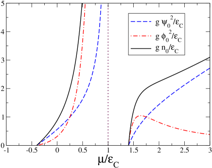
Figure 1: (Color online). Scaled effective densities of the uniform exciton-polariton condensate versus the scaled chemical potential, $\mu/\epsilon_{C}$, for the effective (emulated) Rabi coupling $\Gamma=0.75\epsilon_{C}$. Dashed lines: effective exciton density $\psi_{0}^{2}$; dotted-dashed lines: the respective cavity-photon density $\phi_{0}^{2}$; solid lines: total density $n_{0}$. Other parameters are the effective exciton-exciton repulsion strength $g$, and the exciton and cavity-photon energies, $\epsilon_{X}=0$ and $\epsilon_{C}$ (actually emulated by the propagating-constant shifts in the dual-core waveguide), at zero wavenumber. The curves below and above $\mu/\epsilon_{C}=1$ correspond, respectively, to the lower and upper branches.

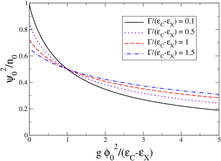
Figure 2: (Color online). Exciton fraction $\psi_{0}^{2}/n_{0}$ in the exciton-polariton condensate as a function of the scaled density of the cavity photons, $g\phi_{0}^{2}/(\epsilon_{C}-\epsilon_{X})$. The four curves correspond to different values of the scaled Rabi coupling, $\Gamma/(\epsilon_{C}-\epsilon_{X})$.

III.2 Modulational instability (MI) of the uniform states

A central point of the analysis is the MI of the flat state which was obtained above. For this purpose, small perturbations ${\eta}_{X}(\mathbf{r},t)$ and ${\eta}_{C}(\mathbf{r},t)$ are added to the uniform fields, $\psi_{0}$ and $\phi_{0}$, by setting

$$\left\{{\psi}(\mathbf{r},t),{\phi}(\mathbf{r},t)\right\}=\left[\left\{\psi_{0},\phi_{0}\right\}+\left\{{\eta}_{1}(\mathbf{r},t),{\eta}_{2}(\mathbf{r},t)\right\}\right]\ e^{-i\mu t}\;.$$ (11)

The subsequent linearization of Eqs. (1) and (2) gives

$$i{\frac{\partial}{\partial t}}{\eta}_{1} = \left(-{\frac{1}{2m_{X}}}\nabla_{\bot}^{2}+\mu_{X}-2{\frac{\Gamma^{2}}{\mu_{C}}}\right){\eta}_{1}$$

$$+ (\mu_{X}-{\frac{\Gamma^{2}}{\mu_{C}}})\ {\eta}_{1}^{\ast}+\Gamma{\eta}_{2}\;,$$

$$i{\frac{\partial}{\partial t}}{\eta}_{2} = \left(-{\frac{1}{2m_{C}}}\nabla_{\bot}^{2}-\mu_{C}\right){\eta}_{2}+\Gamma{\eta}_{1}\;,$$ (12)

where we have defined

$$\mu_{X}\equiv\mu-\epsilon_{X},\quad\quad\mu_{C}\equiv\mu-\epsilon_{C}.$$ (13)

Solution to linearized equations (12) are looked for as

$$\eta_{1}(\mathbf{r},t) = A_{1}\ e^{i(\mathbf{k}\cdot\mathbf{r}-\omega_{k}t)}+B_{1}\ e^{-i(\mathbf{k}\cdot\mathbf{r}-\omega_{k}t)}\;,$$ (14)

$$\eta_{2}(\mathbf{r},t) = A_{2}\ e^{i(\mathbf{k}\cdot\mathbf{r}-\omega_{k}t)}+B_{2}\ e^{-i(\mathbf{k}\cdot\mathbf{r}-\omega_{k}t)}\;,$$ (15)

where $\mathbf{k}$ and $\omega_{k}$ are the wave vector and frequency of the perturbations. It is straightforward to derive a dispersion relation from Eqs. (14) and (15):

$$\omega_{k}^{\pm}=\sqrt{-\beta\pm\sqrt{\beta^{2}-4\gamma}},$$ (16)

where additional combinations are defined:

$$\beta \equiv -(a^{2}-b^{2}+c^{2}+2\Gamma^{2}),~{}$$ (17)

$$\gamma \equiv a^{2}c^{2}-b^{2}c^{2}-2ac\Gamma^{2}+\Gamma^{4},$$ (18)

$$a \equiv k^{2}/(2m_{X})+\mu_{X}-2\Gamma^{2}/\mu_{C},~{}$$ (19)

$$b \equiv \mu_{x}-\Gamma^{2}/\mu_{C},$$ (20)

$$~{}c \equiv k^{2}/(2m_{C})-\mu_{C}.$$ (21)

In the absence of the effective Rabi coupling, i.e., in the case of the uncoupled waveguiding cores ($\Gamma=0$), branch $\omega_{k}^{-}$ in Eq. (16) gives the familiar gapless Bogoliubov-like spectrum,

$$\omega_{k}=\sqrt{{\frac{k^{2}}{2m_{X}}}\left({\frac{k^{2}}{2m_{X}}}+2\,\mu_{X}\right)},$$ (22)

while $\omega_{k}^{+}$ yields

$$\omega_{k}=\left|{\frac{k^{2}}{2m_{C}}}-\mu_{C}\right|,$$ (23)

which may be realized as a gapped spectrum. It is easy to verify that branches (22) and (23) do not intersect, provided that $\epsilon_{X}<\mu<\epsilon_{C}$. Notice that for $\Gamma=0$ one has $\epsilon_{X}=\mu_{0}^{-}$, see Eq. (8). In the presence of the effective Rabi coupling ($\Gamma\neq 0$), emulated by the coupling between the parallel cores, frequencies (16) acquire a finite imaginary part under the condition of $\mu>\epsilon_{C}$. This means that the uniform state pertaining to the upper branch of the dispersion relation, i.e., $\mu^{+}$ in Eq. (8), is always unstable. Instead, for the uniform state pertaining to the lower branch, characterized by $\mu^{-}$ in Eq. (8), perturbation eigenfrequencies (16) are always real. Indeed, in the experiments with the EP condensates, only the lower polariton branch is actually observed.

Dealing with the stability region, in Fig. 2 we plot the effective exciton fraction, $\psi_{0}^{2}/n_{0}$, of the EP-emulating state as a function of the effective scaled cavity-photon density, $g\phi_{0}^{2}/(\epsilon_{C}-\epsilon_{X})$, at four values of the scaled coupling: $\Gamma/(\epsilon_{C}-\epsilon_{X})=0.1,~{}0.5,1,1.5$ (solid, dotted, dashed, and dotted-dashed lines, respectively). The figure shows that the exciton fraction decreases with the increase of $\phi_{0}^{2}$, while, at a fixed value of $\phi_{0}^{2}$, this fraction slightly grows with $\Gamma$. In addition, from Fig. 2, and also from Eqs. (6) and (7), one finds that the uniform state has equal effective densities of excitons and cavity photons, i.e., $\psi_{0}^{2}/n_{0}=1/2$, at $g\phi_{0}^{2}=\epsilon_{C}-\epsilon_{X}$.

III.3 Collective excitations

The uniform state is stable in the regime where frequencies (16) are real, i.e., as said above, for the lower branch of the nonlinear dispersion relation. Here we aim to analyze dispersion relations for collective excitations on top of the stable uniform state.

In the previous section, it was demonstrated that, in the absence of the linear coupling ($\Gamma=0$), frequencies (16) split into two branches, the gapless Bogoliubov-like one (22), and its gapped counterpart (23). In the presence of the coupling ($\Gamma\neq 0$), the two branches can be identified: the Bogoliubov-like spectrum, $\omega_{k}^{-}$, given by Eq. (16), is gapless, i.e. $\omega_{0}^{-}=0$, while Eq. (16) yields the gapped spectrum, $\omega_{k}^{+}$, with $\omega_{0}^{+}\neq 0$.

As mentioned above, the effective exciton and cavity-photon masses are widely different in the physically relevant setting, $m_{X}\gg m_{C}$, therefore in many case it is possible to simplify the problem by setting $1/m_{X}=0$ rev-francesca ; rev-iacopo . In this limit case, Eq. (16) yields the first-sound velocity $c_{s}$, obtained by the expansion of the Bogoliubov-like spectrum, $\omega_{k}^{-}$, at small $k$, $\omega_{k}^{-}\approx c_{s}\,k,$ with

$$c_{s}=\sqrt{{\frac{\epsilon_{C}-\mu}{2m_{C}}}\left[1-{\frac{(\mu_{C}^{2}+\Gamma^{2})^{2}}{\mu_{C}^{4}+2(\mu_{C}^{2}-\mu_{C}\mu_{X})\Gamma^{2}+3\Gamma^{4}}}\right]}.$$ (24)

In the same case, the gap of branch $\omega_{k}^{+}$ is

$$\omega_{0}^{+}=\sqrt{\mu_{C}^{2}+2{\frac{\epsilon_{C}-\epsilon_{X}}{\epsilon_{C}-\mu}}\Gamma^{2}+3{\frac{\Gamma^{4}}{\mu_{C}^{2}}}}\;.$$ (25)

In Fig. 3 we plot the scaled energy, $m_{C}c_{s}^{2}/(\epsilon_{C}-\epsilon_{X})$, of the first-sound mode (the upper panel), and the scaled energy gap, $\omega_{0}^{+}/(\epsilon_{C}-\epsilon_{X})$, of the gapped branch (the lower panel), as functions of the scaled effective cavity-photon density, $g\phi_{0}^{2}/(\epsilon_{C}-\epsilon_{X})$. Four curves in each panel correspond to different values of the scaled linear coupling, $\Gamma/(\epsilon_{C}-\epsilon_{X})$: $0.1,0.5,1,1.5$.

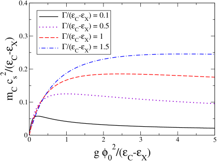
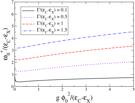
Figure 3: (Color online). The top panel: scaled energy $m_{C}c_{s}^{2}/(\epsilon_{C}-\epsilon_{X})$ of the first-sound mode, with the sound speed $c_{s}$, versus the scaled effective cavity-photon density, $g\phi_{0}^{2}/(\epsilon_{C}-\epsilon_{X})$. The bottom panel: scaled energy gap $\omega_{0}^{+}/(\epsilon_{C}-\epsilon_{X})$ of the gapped branch versus the scaled cavity-photon density. In each panel, four curves correspond to different values of the scaled linear coupling, $\Gamma/(\epsilon_{C}-\epsilon_{X})$.

It is relevant to simulate the evolution of the stable uniform state excited by a small circular perturbation, which corresponds to an experimentally relevant situation. In Fig. 4 we display the evolution produced by simulations of Eqs. (1) and (2), using a 2D real-time Crank-Nicolson method with the predictor-corrector element and periodic boundary conditions sala-numerics . For this purpose, we choose the following initial conditions:

$$\psi(x,t=0) = \psi_{0},$$ (26)

$$\phi(x,t=0) = \phi_{0}+A~{}e^{-(x^{2}+y^{2})/\sigma^{2}},$$ (27)

where $\psi_{0}$ and $\phi_{0}$ are solutions of Eqs. (6) and (7), while $A$ and $\sigma$ are parameters of the perturbation, which represents a small circular hole. We here set $\epsilon_{X}=0$, $\epsilon_{C}=1$, $g=1$, $\Gamma=0.75$, $m_{X}=1000$ and $m_{C}=1$. Figure 4 displays the spatial profile of the perturbed condensate density, $n_{0}(x,t)=|\psi(x,t)|^{2}+|\phi(x,t)|^{2}$, at different values of the propagation distance (time, in terms of EP), $t=9$, $t=12$, $t=21$, for initial perturbation (27) with $A=0.1$ and $\sigma=2$. In the case shown in Fig. 4 the unperturbed amplitudes are $\psi_{0}=1$ and $\phi_{0}=-1$, which correspond in Fig. 1 to $\mu=0.25$ (the lower branch). As observed in Fig. 4, the initial perturbation produces a circular pattern which expands with a radial velocity close to the speed of sound, $c_{s}$ (for further technical details, see Ref. sala-shock ).

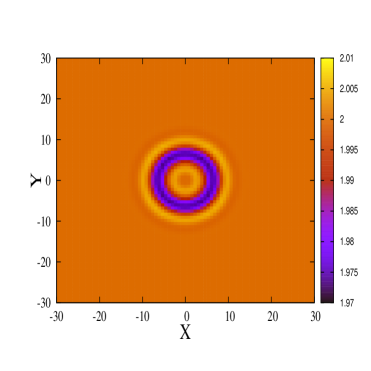
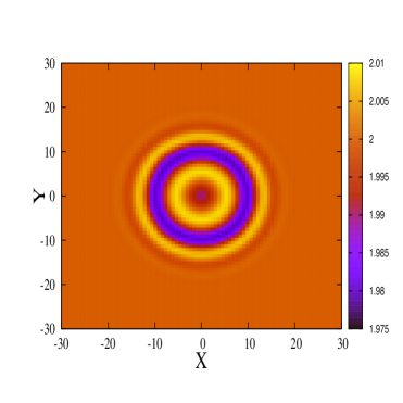
Figure 4: (Color online). The evolution of the initial circular perturbation in the form of a small hole produced on top of the stable uniform state, per Eqs. (26) and (27). Each panel displays contour plots of the total density, $n_{0}(x,y,t)$, at fixed values of the propagation distance (effective time), $t.$ The top, middle, and bottom panels correspond to $t=9$, $t=15$, and $t=21$, respectively. Parameters are $\epsilon_{X}=0$, $\epsilon_{C}=1$, $g=1$, $\Gamma=0.75$. Initial conditions are taken as in Eqs. (26) and (27) with $\psi_{0}=1$, $\phi_{0}=-1$, $A=0.1$ and $\sigma=2$.

We have also simulated the evolution of unstable configurations – for instance, with unperturbed amplitudes $\psi_{0}=1$ and $\phi_{0}=1$, which correspond to $\mu=1.75$, i.e., the upper branch in Fig. 1. The evolution is initially similar to that shown in Fig. 4, but later a completely different behavior is observed, with the formation of several circles whose amplitude strongly grows in the course of the unstable evolution.

IV The uniform condensate with a phase gradient

We now analyze the existence and stability of a uniform state with a phase gradient (effective superflow), which corresponds to setting

$$\left\{{\psi}(\mathbf{r},t),{\phi}(\mathbf{r},t)\right\}=\left\{\psi_{0},\phi_{0}\right\}e^{i(\mathbf{q}\cdot\mathbf{r}-\mu t)}$$ (28)

in Eqs. (1) and (2), where $\mathbf{q}=(q_{x},q_{y})$ is the wave vector of the gradient, with $\psi_{0}$ and $\phi_{0}$ given by

$$\psi_{0}^{2} = {\frac{1}{g}}\left({\tilde{\mu}}_{X}-{\frac{\Gamma^{2}}{{\tilde{\mu}}_{C}}}\right)\;,$$ (29)

$$\phi_{0} = -{\frac{\Gamma}{{\tilde{\mu}}_{C}}}\,\psi_{0}~{},$$ (30)

where

$${\tilde{\mu}}_{X}=\mu-\epsilon_{X}-{\frac{q^{2}}{2m_{X}}}~{},~{}\ {\tilde{\mu}}_{C}=\mu-\epsilon_{C}-{\frac{q^{2}}{2m_{C}}}\;.$$ (31)

Following the same procedure as developed in the previous section, we derive the quartic dispersion equation,

$$\alpha_{4}\omega_{\mathbf{k}}^{4}+\alpha_{3}\omega_{\mathbf{k}}^{3}+\alpha_{2}\omega_{\mathbf{k}}^{2}+\alpha_{1}\omega_{\mathbf{k}}+\alpha_{0}=0\;,$$ (32)

for frequencies $\omega_{k}$ of small excitations on top of the uniform state. Here we define

$$\alpha_{0} = a_{1}a_{2}c_{1}c_{2}-b^{2}c_{1}c_{2}-a_{1}c_{1}\Gamma^{2}-a_{2}c_{2}\Gamma^{2}+\Gamma^{4}\;,$$

$$\alpha_{1} = a_{1}a_{2}c_{1}-b^{2}c_{1}-a_{1}a_{2}c_{2}+b^{2}c_{2}+a_{1}c_{1}c_{2}$$

$$- a_{2}c_{1}c_{2}+a_{1}\Gamma^{2}-a_{2}\Gamma^{2}\;,$$

$$\alpha_{2} = -a_{1}a_{2}+b^{2}+a_{1}c_{1}-a_{2}c_{1}-a_{1}c_{2}$$

$$+ a_{2}c_{2}-c_{1}c_{2}-2\Gamma^{2}\;,$$

$$\alpha_{3} = -a_{1}+a_{2}-c_{1}+c_{2}\;,$$

$$\alpha_{4} = 1\;,$$

$$a_{1} = k^{2}/(2m_{X})+{\tilde{\mu}}_{X}-2\Gamma^{2}/{\tilde{\mu}}_{C}+\mathbf{q}\cdot\mathbf{k}/m_{X}\;,$$

$$a_{2} = k^{2}/(2m_{X})+{\tilde{\mu}}_{X}-2\Gamma^{2}/{\tilde{\mu}}_{C}-\mathbf{q}\cdot\mathbf{k}/m_{X}\;,$$

$$b = {\tilde{\mu}}_{X}-\Gamma^{2}/{\tilde{\mu}}_{C}\;,$$

$$c_{1} = k^{2}/(2m_{C})+{\tilde{\mu}}_{C}+\mathbf{q}\cdot\mathbf{k}/m_{C}\;,$$

$$c_{2} = k^{2}/(2m_{C})+{\tilde{\mu}}_{C}-\mathbf{q}\cdot\mathbf{k}/m_{C}\;.$$

In the absence of the linear coupling ($\Gamma=0$), Eq. (32) gives the $\mathbf{q}$-dependent gapless Bogoliubov-like spectrum,

$$\omega_{\mathbf{k}}={\frac{\mathbf{q}\cdot\mathbf{k}}{m_{X}}}\pm\sqrt{{\frac{k^{2}}{2m_{X}}}\left({\frac{k^{2}}{2m_{X}}}+2\,\left(\mu_{X}-{\frac{q^{2}}{2m_{X}}}\right)\right)},$$ (33)

and the $\mathbf{q}$-dependent gapped one,

$$\omega_{\mathbf{k}}={\frac{\mathbf{q}\cdot\mathbf{k}}{m_{C}}}\pm\left|{\frac{k^{2}+q^{2}}{2m_{C}}}-\mu_{C}+{\frac{q^{2}}{2m_{C}}}\right|.$$ (34)

In the presence of the linear coupling ($\Gamma\neq 0$) one must solve Eq. (32) numerically. We direct the $x$ axis along $\mathbf{q}$, hence $\mathbf{q}=(q,0)$. In Fig. 5 we plot frequencies $\omega_{(k,0)}$ of longitudinal perturbations, with wave vector $\mathbf{k}=\left(k,0\right)$, for three different values of the flux wavenumber, $q$. For these values of $q$, the imaginary part of frequencies $\omega_{(k,0)}$ is zero, hence the state is stable. In the first two panels of Fig. 5 (with $q=0$ and $q=0.5$) one clearly sees gapped and gapless modes, which are (approximately) symmetric for $k>0$ and $k<0$, which corresponds to excitation waves moving in opposite directions with equal speeds. By increasing $q$ one reaches the Landau critical wavenumber, $q_{L}\simeq 0.72$, at which the gapless mode has zero frequency at a finite value of $k$, and above which there is a finite range of $k$’s where two gapless modes propagate in the same direction, i.e., the phase velocity, $\omega_{(k,0)}/k$, has the same sign for both the modes. This is shown in the lower panel of Fig. 5 (for $q=1$), where, according to the Landau criterion, the system is not fully superfluid book-leggett . A further increase of $q$ leads to the dynamical instability of the gapless modes through the appearance of a nonzero imaginary part of $\omega_{(k,0)}$, as shown in Fig. 6, where both real and imaginary parts of $\omega_{(k,0)}$ are displayed for $q=1.5$. Actually, the sound velocities of the two gapless modes moving in the same direction become equal, so that they may exchange energy and therefore become unstable, at the critical flux wavenumber $q_{c}\simeq 1.15$. The results reported in Fig. 5 and 6 are obtained from calculations performed at constant $\mu$. We have verified that the same phenomenon occurs as well at fixed values of the total density.

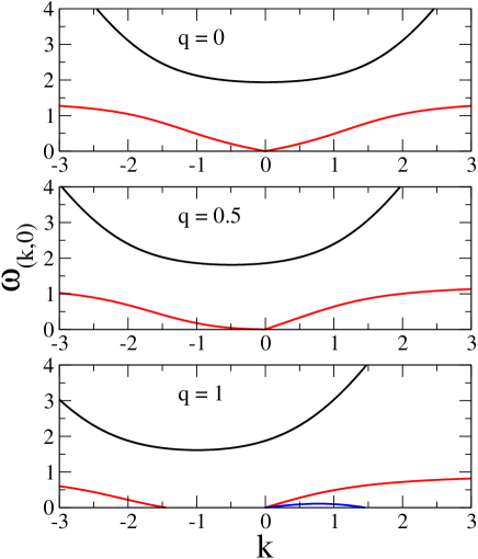
Figure 5: (Color online). Frequencies of small excitations $\omega_{(k,0)}$ above the stable uniform state with wave vector $\mathbf{q}=(q,0)$ of the phase flux. Parameters are $\epsilon_{X}=0$, $\epsilon_{C}=1$, $g=1$, $\Gamma=0.75$, $m_{X}=1000$, $m_{C}=1$, and $\mu=0.25$. Each line corresponds to a different solution (branch) of Eq. (32).

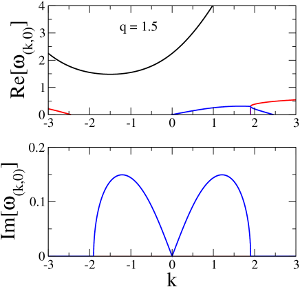
Figure 6: (Color online). Real and imaginary parts, $\mathrm{Re}[\omega_{k}]$ and $\mathrm{Im}[\omega_{k}]$, of excitation frequencies $\omega_{k}$ on top of the unstable uniform state with wave vector $\mathbf{q}=\left(1.5,0\right)$ of the phase flux. Parameters are $\epsilon_{X}=0$, $\epsilon_{C}=1$, $\gamma=1$, $\Gamma=0.75$, $m_{X}=1000$, $m_{C}=1$, and $\mu=0.25$. Each line corresponds to a different solution (branch) of Eq. (32).

V Reduction to the one-dimensional system

As said above, the 1D lossless EP system may be straightforwardly emulated by the dual-core optical fiber, in which one core is nonlinear, operating near the zero-GVD point, while the other one is linear, carrying nonzero GVD. The accordingly simplified version of Eqs. (1) and (2) is written as

$$i{\frac{\partial}{\partial t}}{\tilde{\psi}} = \left[\epsilon_{X}+g\,|{\tilde{\psi}}|^{2}\right]{\tilde{\psi}}+\Gamma\ {\tilde{\phi}}\;,$$ (35)

$$i{\frac{\partial}{\partial t}}{\tilde{\phi}} = \left[-{\frac{1}{2m_{C}}}{\frac{\partial^{2}}{\partial x^{2}}}+\epsilon_{C}+V(x)\right]{\tilde{\phi}}+\Gamma\ {\psi}\;,$$ (36)

where the tildes stress the reduction to 1D.

V.1 Stability of the uniform 1D state

The results shown in Figs. 1 and 2 are also valid in 1D, taking into regard that $\psi_{0}^{2}$ and $\phi_{0}^{2}$ are now 1D densities. In Figs. 7 and 8, we show the evolution of small perturbations on top of the uniform stable and unstable states, respectively. For this purpose, Eqs. (1) and (2) were simulated by means of the 1D real-time Crank-Nicolson algorithm with the use of the predictor-corrector element sala-numerics . The initial conditions were taken as

$${\tilde{\psi}}(x,t=0) = \psi_{0}\;,$$ (37)

$${\tilde{\phi}}(x,t=0) = \phi_{0}+A~{}e^{-x^{2}/\sigma^{2}}.$$ (38)

In both Figs. 7 and 8, the same parameters of the system are used: $\epsilon_{X}=0$, $\epsilon_{C}=1$, $g=1$, $\Gamma=0.75$. Both figures 7 and 8 display spatial profiles of the condensate density, $n_{0}(x,t)=|{\tilde{\psi}}(x,t)|^{2}+|{\tilde{\phi}}(x,t)|^{2}$, at different values of the propagating constant (alias time, in terms of the EP system), $t=0$, $t=3$, $t=9$, $t=12$, generated by the initial perturbation (38), with $A=-0.1$ and $\sigma=2$. In Fig. 7, the unperturbed amplitudes are $\psi_{0}=1$ and $\phi_{0}=-1$, which correspond to $\mu=0.25$, i.e., the lower branch in terms of Fig. 1, while in Fig. 8 the initial amplitudes are $\psi_{0}=1$ and $\phi_{0}=1$, corresponding to $\mu=1.75$ on the upper branch.

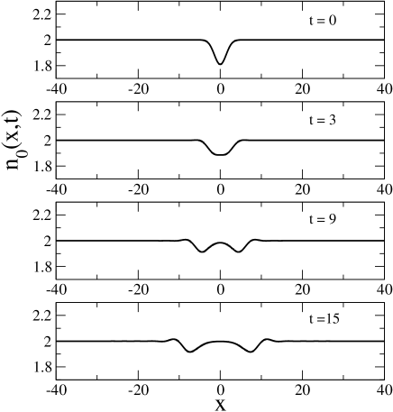
Figure 7: (Color online) The evolution of a small hole produced, as a perturbation, on top of a stable uniform 1D state. In each panel, density profiles $n\left(x,t\right)$ are displayed. Parameters are: $\epsilon_{X}=0$, $\epsilon_{C}=1$, $g=1$, $\Gamma=0.75$. Initial conditions are given by Eqs. (26) and (27) with $\psi_{0}=1$, $\phi_{0}=-1$, $A=0.1$ and $\sigma=2$.

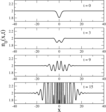
Figure 8: (Color online) The evolution of a small hole produced, as a perturbation, on top of an unstable 1D state. Parameters are $\epsilon_{X}=0$, $\epsilon_{C}=1$, $g=1$, $\Gamma=0.75$. Initial conditions are given by Eqs. (26) and (27) with $\psi_{0}=1$, $\phi_{0}=1$, $A=-0.1$ and $\sigma=2$.

As seen in Fig. 7, the initial perturbation hole splits into two ones traveling in opposite directions with a velocity close to the speed of sound $c_{s}$ (see further technical details in Ref. sala-shock ). In Fig. 8, the dynamics is initially (at $t\leq 6$) similar to that in Fig. 7, but at $t>6$ it displays a completely different behavior, namely, formation of strong oscillations, which increase their amplitude in the course of the evolution, indicating a dynamical instability.

V.2 One-dimensional dark solitons , and a possibility of the existence of vortices in the 2D system

In the case when the 1D uniform background is stable, it is natural to look for solutions in the form of dark solitons (DSs). As well as in other systems, the node at the center of the DS is supported by a phase shift of $\pi$ between the wave fields at $x\rightarrow\pm\infty$ Dark (as shown below, in the present system the node and the phase shift by $\pi$ exist simultaneously in both fields, $\psi$ and $\phi$).

To demonstrate the possibility of the existence of the DS, we substitute the general 1D ansatz for stationary solutions into Eqs. (35) and (36):

$$\left\{{\tilde{\psi}}(x,t),{\tilde{\phi}}(x,t)\right\}=\left\{\Psi(x),\Phi(x)\right\}\ e^{-i\mu t}\;,$$ (39)

with functions $\Psi(x)$ and $\Phi(x)$, which may be assumed real, obeying the coupled stationary equations:

$$\Gamma\,\Phi=\left(\mu-\epsilon_{X}\right){\Psi}-g\,\Psi^{3},$$ (40)

$$\left(\mu-\epsilon_{C}\right){\Phi}+\frac{1}{2m_{C}}\Phi^{\prime\prime}-\Gamma\ {\Psi}=0,$$ (41)

where approximation $1/m_{X}=0$ is adopted, and $\Phi^{\prime\prime}\equiv d^{2}\Phi/dx^{2}$. It is straightforward to check that Eqs. (40) and (41) admit a solution with $\Psi(x)=-\Phi(x)$ only if ${\Phi}^{\prime\prime}\equiv 0$ for any $x$, i.e., DS solutions do not obey this constraint.

For the analytical consideration, we assume that the second derivative in Eq. (41) may be treated as a small term. Then, an approximate solution of Eq. (41) is

$$\Phi\approx-\frac{\Gamma}{\epsilon_{C}-\mu}\Psi-\frac{\Gamma}{2m_{C}\left(\epsilon_{C}-\mu\right)^{2}}\Psi^{\prime\prime}\;,$$ (42)

and the substitution of expression (42) into Eq. (40) leads to the following equation for $\Psi(x)$:

$$-\frac{\Gamma^{2}}{2m_{C}\left(\epsilon_{C}-\mu\right)^{2}}\Psi^{\prime\prime}+g\Psi^{3}-\left[\left(\mu-\epsilon_{X}\right)+\frac{\Gamma^{2}}{\left(\epsilon_{C}-\mu\right)}\right]\Psi=0.$$ (43)

Equation (43) yields a commonly known exact dark-soliton solution:

$$\Psi(x) =\pm\sqrt{\frac{1}{g}\left[\left(\mu-\epsilon_{X}\right)+\frac{\Gamma^{2}}{\left(\epsilon_{C}-\mu\right)}\right]}$$

$$\times \tanh\left(\frac{1}{\Gamma}\sqrt{m_{C}\left(\epsilon_{C}-\mu\right)\left[\left(\mu-\epsilon_{X}\right)\left(\epsilon_{C}-\mu\right)+\Gamma^{2}\right]}x\right)\;.$$ (44)

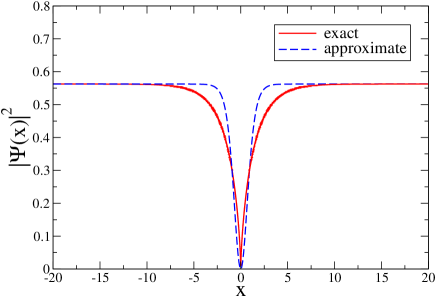
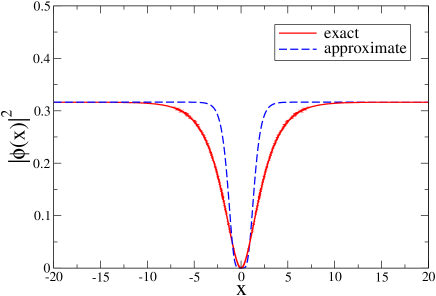
Figure 9: (Color online) The dark soliton for $\epsilon_{X}=\mu=0$, $\epsilon_{C}=1$, $\gamma=1$, $\Gamma=0.75$. The exact solution (solid line) is produced by Eq. (48), and its approximate counterpart (dashed line) is given by Eq. (44). The top and bottom panels display the excitonic and photonic density profiles, $|\Psi(x)|^{2}$ and $|\Phi(x)|^{2}$, respectively.

On the other hand, in the special case of $\mu=\epsilon_{X}$, Eq. (40) can be used to eliminate $\Phi$ in favor of $\Psi$:

$$\Phi=-\left(g/\Gamma\right)\Psi^{3},$$ (45)

the remaining equation for $\chi\equiv\Psi^{3}$ being

$$\frac{1}{2m_{C}}\frac{d^{2}\chi}{dx^{2}}=\left(\epsilon_{C}-\epsilon_{X}\right)\chi-\frac{\Gamma^{2}}{g}\chi^{1/3}.$$ (46)

If $x$ is formally considered as time, Eq. (46) is the Newton’s equation of motion for a particle in an effective external potential,

$$U_{\mathrm{eff}}(\chi)=\frac{3\Gamma^{2}}{4g}\chi^{4/3}-\frac{1}{2}\left(\epsilon_{C}-\epsilon_{X}\right)\chi^{2}.$$ (47)

It is obvious that this potential gives rise to a heteroclinic trajectory which connects two local maxima of potential (47), $\chi_{0}=\pm\left[\Gamma^{2}/\left(g\left(\epsilon_{C}-\epsilon_{X}\right)\right)\right]^{3/2}$. An implicit analytical form of $\chi(x)$ for the corresponding solution given by

$$x=\int_{0}^{\chi(x)}d\xi\sqrt{\frac{2}{\left(4s_{1}^{3}/27s_{0}^{2}\right)+s_{0}\xi^{2}-s_{1}\xi^{4/3}}}\;,$$ (48)

where $s_{0}=m_{C}(\epsilon_{C}-\epsilon_{X})$ and $s_{1}=3m_{C}\Gamma^{2}/(2g)$. From $\chi(x)$ one obtains $\Psi(x)=\left[\chi(x)\right]^{1/3}$ and $\Phi(x)=-(g/\Gamma)\chi(x)$. In Fig. 9 we compare the exact implicit DS solution (solid line), produced by Eq. (48), and its approximate counterpart (dashed line) given by Eq. (44).

Finally, getting back to the full 2D system of Eqs. (1) and (2), and substituting there $\left\{{\psi}(\mathbf{r},t),{\phi}(\mathbf{r},t)\right\}=\left\{\Psi(\mathbf{r}),\Phi(\mathbf{r})\right\}e^{-i\mu t}$, cf. Eq. (39), we note that the existence of 2D vortices can be predicted by means of the approximation similar to that in Eq. (42), i.e.,

$$\Phi\approx-\frac{\Gamma}{\epsilon_{C}-\mu}\Psi-\frac{\Gamma}{2m_{C}\left(\epsilon_{C}-\mu\right)^{2}}\nabla_{\perp}^{2}\Psi.$$ (49)

The substitution of this into the stationary version of Eq. (1) with $1/m_{X}=0$ yields

$$-\frac{\Gamma^{2}}{2m_{C}\left(\epsilon_{C}-\mu\right)^{2}}\nabla_{\perp}^{2}\Psi+g\left|\Psi\right|^{2}\Psi$$

$$-\left[\left(\mu-\epsilon_{X}\right)+\frac{\Gamma^{2}}{\left(\epsilon_{C}-\mu\right)}\right]\Psi=0,$$ (50)

cf. Eq. (43). It is the usual 2D nonlinear Schrödinger equation with the self-defocusing nonlinearity, which gives rise to commonly known vortex states vortices .

VI Conclusions

The objective of this work is to propose the dual-core optical waveguide, with one linear and one dispersive cores, as an emulator for the EP (exciton-polariton) system in the lossless limit, which is not currently achievable in semiconductor microcavities. In terms of this model, the first fundamental issue is the MI (modulational instability) of the uniform state. As might be expected, it is found that the uniform states corresponding to the upper and lower branches of the nonlinear dispersion relation are, respectively, unstable and stable. This analytical result is confirmed by direct simulations, which demonstrate the evolution of localized perturbations on top of stable and unstable backgrounds. The excitation modes supported by the stable background are analyzed too, demonstrating two gapless and gapped branches in the spectrum. The stability investigation was generalized for the uniform background with the phase flux, demonstrating that the lower-branch state loses the stability at the critical value of the flux wavenumber. Finally, approximate and exact analytical solutions for stable dark solitons supported by the 1D setting are produced too.

The analysis may be extended in other directions. In particular, a challenging problem is an accurate investigation of 2D vortices, the existence of which is suggested by the approximate equation (50).

References

- (1) P. Hauke, F. M. Cucchietti, L. Tagliacozzo, I. Deutsch, and M. Lewenstein, Rep. Prog. Phys. 75, 082401 (2012).
- (2) C. J. Pethick and H. Smith, Bose-Einstein Condensation in Dilute Gases (Cambridge University Press: Cambridge, 2008).
- (3) S. Giorgini, L. P. Pitaevskii, and S. Stringari, Rev. Mod. Phys. 80, 1215 (2008); X.-W. Guan, M. T. Batchelor, and C. Lee, Rev. Mod. Phys. 85, 1635 (2013).
- (4) Y. J. Lin, K. Jimenez-Garcia, and I. B. Spielman, Nature 471, 83 (2011).
- (5) Y. Zhang, L. Mao, and C. Zhang, Phys. Rev. Lett. 108, 035302 (2012).
- (6) H. Zhai, Int. J. Mod. Phys. B 26, 1230001 (2012).
- (7) Y.-J. Lin, R. L. Compton, A. R. Perry, W. D. Phillips, J. V. Porto, and I. B. Spielman, Phys. Rev. Lett. 102, 130401 (2009); Y.-J. Lin, R. L. Compton, K. Jiménez-García, J. V. Porto, and I. B. Spielman, Nature 462, 628 (2009); T.-L. Ho and S. Zhang, Phys. Rev. Lett. 107, 150403 (2011).
- (8) J. Dalibard, F. Gerbier, G. Juzeliunas, and P. Öhberg, Rev. Mod. Phys. 83, 1523 (2011); N. Goldman, G. Juzeliuunas, P. Öhberg, and I. B. Spielman, arXiv:1308.6533v1.
- (9) T. Schwartz, G. Bartal, S. Fishman, and M. Segev, Nature 446, 52 (2007); Y. Lahini, A. Avidan, F. Pozzi, M. Sorel, R. Morandotti, D. N. Christodoulides, and Y. Silberberg, Phys. Rev. Lett. 100, 013906 (2008).
- (10) J. Billy, V. Josse, Z. Zuo, A. Bernard, B. Hambrecht, P. Lugan, D. Clement, L. Sanchez-Palencia, P. Bouyer, and A. Aspect, Nature 453, 891 (2008); G. Roati, C. D’Errico, L. Fallani, M. Fattori, C. Fort, M. Zaccanti, G. Modugno, M. Modugno, and M. Inguscio, Nature 453, 895 (2008).
- (11) M. C. Rechtsman, Y. Plotnik, J. M. Zeuner, D. H. Song, Z. G. Chen, A. Szameit, and M. Segev, Phys. Rev. Lett. 111, 103901 (2013).
- (12) M. C. Rechtsman, J. M. Zeuner, Y. Plotnik, Y. Lumer, D. Podolsky, F. Dreisow, S. Nolte, M. Segev, and A. Szameit, Nature 496, 196 (2013).
- (13) A. Ruschhaupt, F. Delgado, and J. G. Muga, J. Phys. A 38, L171 (2005); K. G. Makris, R. El-Ganainy, D. N.Christodoulides, and Z. H. Musslimani, Phys. Rev. Lett. 100, 103904 (2008); S. Longhi, Phys. Rev. A 81, 022102 (2010); C. E. Rüter, K. G. Makris, R. El-Ganainy, D. N. Christodoulides, M. Segev, and D. Kip, Nat. Phys. 6, 192 (2010).
- (14) K. G. Makris, R. El-Ganainy, D. N. Christodoulides, and Z. H. Musslimani, Int. J. Theor. Phys. 50, 1019 (2011).
- (15) F. Dreisow, M. Heinrich, R. Keil, A. Tünnermann, S. Nolte, S. Longhi, and A. Szameit, Phys. Rev. Lett. 105, 143902 (2010).
- (16) S. Longhi, Laser and Photonic Reviews 3, 243 (2009).
- (17) V. Achilleos, D. J. Frantzeskakis, P. G. Kevrekidis, and D. E. Pelinovsky, Phys. Rev. Lett. 110, 264101 (2013).
- (18) B. A. Malomed, Phys. Rev. A 43, 410 (1991).
- (19) K. E. Strecker, G. B. Partridge, A. G. Truscott, and R. G. Hulet, New J. Phys. 5, 73.1 (2003); F. Kh. Abdullaev, A. Gammal, A. M. Kamchatnov, and L. Tomio, Int. J. Mod. Phys. B 19, 3415 (2005); O. Morsch and M. Oberthaler, Rev. Mod. Phys. 78, 179 (2006).
- (20) B. Deveaud (Ed.), The Physics of Semiconductor Microcavities: From Fundamentals to Nanoscale Devices (Wiley-VCH, Weinheim, 2007).
- (21) A. Kavokin, J. J. Baumberg, G. Malpuech, F. P. Laussy, Microcavities (Oxford University Press, 2007).
- (22) J. Keeling, F. M. Marchetti, M. H. Szymanska, and P. B. Littlewood, Semicond. Sci. Technol. 22, R1 (2007).
- (23) I. Carusotto and C. Ciuti, Rev. Mod. Phys. 85, 299 (2013).
- (24) A. Baas, J. Ph. Karr, H. Eleuch, E. Giacobino, Phys. Rev. A 69, 023809 (2004).
- (25) N. A. Gippius, S. G. Tikhodeev, V. D. Kulakovskii, D. N. Krizhanovskii, A. I. Tartakovskii, Europhys. Lett. 67, 997 (2004).
- (26) I. Carusotto, C. Ciuti, Phys. Rev. Lett. 93, 166401 (2004).
- (27) P. G. Savvidis, J. J. Baumberg, R. M. Stevenson, M. S. Skolnick, D. M. Whittaker, J. S. Roberts, Phys. Rev. Lett. 84, 1547 (2000).
- (28) A. Amo, D. Sanvitto, F. P. Laussy, D. Ballarini, E. del Valle, M. D. Martin, A. Lemaitre, J. Bloch, D. N. Krizhanovskii, M. S. Skolnick, C. Tejedor, L. Viña, Nature 457, 291 (2009).
- (29) A. M. Kamchatnov, S. A. Darmanyan, M. Neviere, J. of Luminescence 110, 373 (2004).
- (30) A. V. Yulin, O. A. Egorov, F. Lederer, D. V. Skryabin, Phys. Rev. A 78, 061801(R) (2008).
- (31) O. A. Egorov, D. V. Skryabin, A. V. Yulin, F. Lederer, Phys. Rev. Lett. 102, 153904 (2009).
- (32) L. A. Smirnov, D. A. Smirnova, E. A. Ostrovskaya, and Y. S. Kivshar, arXiv:1404.1742.
- (33) M. Sich, D. N. Krizhanovskii, M. S. Skolnick, A. V. Gorbach, R. Hartley, D. V. Skryabin, E. A. Cerda-Méndez, K. Biermann, R. Hey and P. V. Santos, Nature Phot. 6, 50 (2012).
- (34) M. Sich, F. Fras, J. K. Chana, M. S. Skolnick, and D. N. Krizhanovskii, A. V. Gorbach, R. Hartley, D. V. Skryabin, S. S. Gavrilov, E. A. Cerda-Méndez, K. Biermann, R. Hey, and P. V. Santos, Phys. Rev. Lett. 112, 046403 (2014).
- (35) A. V. Gorbach, B. A. Malomed, and D. V. Skryabin, Phys. Lett. A 373, 3024 (2009); E. A. Cerda-Méndez, D. Sarkar, D. N. Krizhanovskii, S. S. Gavrilov, K. Biermann, M. S. Skolnick, and P. V. Santos, Phys. Rev. Lett. 111, 146401 (2013).
- (36) J. Kasprak, M. Richard, S. Kundermann, A. Baas, P. Jeambrun, J. M. J. Keeling, F. M. Marchetti, M. H. Szymańska, R. André, J. L. Staehli, V. Savona, P. B. Littlewood, B. Deveaud, and Le Si Dang, Nature 443, 409 (2006).
- (37) S. Utsunomiya, L. Tian, G. Roumpos, C. W. Lai, N. Kumada, T. Fujisawa, M. Kuwata-Gonokami, A. Löffler, S. Höfling, A. Forchel, and Y. Yamamoto, Nature Phys. 4, 700 (2008).
- (38) A. Amo, D. Sanvitto, F. P. Laussy, D. Ballarini, E. del Valle, M. D. Martin, A. Lemaître, J. Bloch, D. N. Krizhanovskii, M. S. Skolnick, C. Tejedor and L. Viña, Nature 457, 291 (2009).
- (39) D. Sanvito, F. M. Marchetti, M. H. Szymańska, G. Tosi, M. Baudisch, F. P. Laussy, D. N. Krizhanovskii, M. S. Skolnick, L. Marrucci, A. Lemaître, J. Bloch, C. Tejedor, and L. Viña, Nature Phys. 6, 527 (2010).
- (40) J. Keeling and N. G. Berloff, Phys. Rev. Lett. 100, 250401 (2008).
- (41) M. Wouters and I. Carusotto, Phys. Rev. Lett. 99, 140402 (2007); M. Wouters and V. Savona, Phys. Rev. B 79, 165302 (2009).
- (42) I. Carusotto and C. Ciuti, Phys. Rev. Lett. 93, 166401 (2004).
- (43) E. Cancellieri, F. M. Marchetti, M. H. Szymanska, and C. Tejedor, Phys. Rev. B 83, 214507 (2011).
- (44) J. Atai and B. A. Malomed, Phys. Rev. E 64, 066617 (2001).
- (45) A. Zafrany, B. A. Malomed, and I. M. Merhasin, Chaos 15, 037108 (2005).
- (46) B. J. Mangan, J. C. Knight, T. A. Birks, P. S. Russell, and A. H. Greenaway, Electr. Lett. 36, 1358 (2000); K. Saitoh, Y. Sato, M. Koshiba, Opt. Exp. 11, 3188 (2003); A. Huttunen and P. Torma, ibid. 13, 627 (2005); Z. Wang, T. Taru, T. A. Birks, and J. C. Knight, ibid. 15, 4795 (2007).
- (47) W. Wang, Y. Wang, K. Allaart, and D. Lenstra, Appl. Phys. B 83, 623 (2006).
- (48) N. C. Panoiu, R. M. Osgood, Jr., and B. A. Malomed, Opt. Lett. 31, 1097 (2006); N.-C. Panoiu, B. A. Malomed, and R. M. Osgood, Jr., Phys. Rev. A 78, 013801 (2008).
- (49) I. Carusotto and C. Ciuti, Phys. Rev. Lett. 93, 166401 (2004); I. A. Shelykh, Y. G. Rubo, G. Malpuech, D. D. Solnyshkov, and A. Kavokin, Phys. Rev. Lett. 97, 066402 (2006); Phys. Rev. B 77, 045314 (2008).
- (50) A. M. Kamchatnov and S. V. Korneev, J. Exp. Theor. Phys. 115, 579 (2012); L. A. Smirnov, D. A. Smirnova, E. A. Ostrovskaya, and Y. S. Kivshar, arXiv:1404.1742.
- (51) A.J. Leggett, Quantum Liquids (Oxford Univ. Press, Oxford, 2006).
- (52) E. Cerboneschi, R. Mannella, E. Arimondo, and L. Salasnich, Phys. Lett. A 249, 495 (1998); G. Mazzarella and L. Salasnich, Phys. Lett. A 373, 4434 (2009).
- (53) L. Salasnich, EPL 96, 40007 (2011).
- (54) L. Salasnich, Laser Phys. 12, 198 (2002); L. Salasnich, A. Parola, and L. Reatto, Phys. Rev. A 65, 043614 (2002).
- (55) Y. S. Kivshar, IEEE J. Quant. Eectr. 29, 250 (1993); D. J. Frantzeskakis, J. Phys. A: Math. Theor. 43, 213001 (2010).
- (56) J. C. Neu, Physica D 43, 385 (1990); G. A. Swartzlander and C. T. Law, Phys. Rev. Lett. 69, 2503 (1992); D. Rozas, C. T. Law, and G. A. Swartzlander, J. Opt. Soc. Am. B 14, 3054 (1997).