Model Reduction of Linear Switched Systems by Restricting Discrete Dynamics

Abstract

We present a procedure for reducing the number of continuous states of discrete-time linear switched systems, such that the reduced system has the same behavior as the original system for a subset of switching sequences. The proposed method is expected to be useful for abstraction based control synthesis methods for hybrid systems.

I INTRODUCTION

A discrete-time linear switched system [11, 19] (abbreviated by DTLSS) is a discrete-time hybrid system of the form

$$\Sigma\left\{\begin{split}&x(t+1)=A_{\sigma(t)}x(t)+B_{\sigma(t)}u(t)\mbox{ and }x(0)=x_{0}\\ &y(t)=C_{\sigma(t)}x(t),\end{split}\right.$$ (1)

where $x(t)\in\mathbb{R}^{n}$ is the continuous state, $y(t)\in\mathbb{R}^{p}$ the continuous output, $u(t)\in\mathbb{R}^{m}$ is the continuous input, $\sigma(t)\in Q=\{1,\ldots,D\}$, $D>0$ is the discrete state (switching signal). $A_{q},B_{q},C_{q}$ are matrices of suitable dimension for $q\in Q$. A more rigorous definition of DTLSSs  will be presented later on. For the purposes of this paper, $u(t)$ and $\sigma(t)$ will be viewed as externally generated signals.

Contribution of the paper Consider a discrete-time linear switched system $\Sigma$ of the form (1), and a set $L$ which describes the admissible set of switching sequences. In this paper, we will present an algorithm for computing another DTLSS

$$\bar{\Sigma}\left\{\begin{split}&\bar{x}(t+1)=\bar{A}_{\sigma(t)}\bar{x}(t)+\bar{B}_{\sigma(t)}u(t)\mbox{ and }\bar{x}(0)=\bar{x}_{0}\\ &\bar{y}(t)=\bar{C}_{\sigma(t)}\bar{x}(t)\end{split}\right.$$ (2)

such that for any switching sequence $\sigma(0)\cdots\sigma(t)=q_{0}\cdots q_{t}\in L$ and continuous inputs $u(0),\ldots,u(t-1)$, the output at time $t$ of (1) equals the output of (2), i.e., $y(t)=\bar{y}(t)$ and the number of state variables of (2) is smaller than that of (1). In short, for any sequence of discrete states from $L$, the input-output behavior of $\Sigma$ and $\bar{\Sigma}$ coincide and the size of $\bar{\Sigma}$ is smaller.

Motivation Realistic plant models of industrial interest tend to be quite large and in general, the smaller is the plant model, the smaller is the resulting controller and the computational complexity of the control synthesis or verification algorithm. This is especially apparent for hybrid systems, since in this case, the computational complexity of control or verification algorithms is often exponential in the number of continuous states [20]. The particular model reduction problem formulated in this paper was motivated by the observation that in many instances, we are interested in the behavior of the model only for certain switching sequences. To illustrate this point, we will consider a number of simple scenarios where the results of the paper could potentially be useful.

(1) Control and verification of DTLSSs   with switching constraints. DTLSSs  with switching constraints occur naturally in a large number of applications. Such systems arise for example when the supervisory logic of the switching law is (partially) fixed. Note that verification or control synthesis of DTLSSs  can be computationally demanding, especially if the properties or control objectives of interest are discrete [5]. The results of the paper could be useful for verification or control of such systems, if the properties of interest or the control objectives depend only on the input-output behavior. In this case, we could replace the original DTLSS  $\Sigma$ by the reduced order DTLSS $\bar{\Sigma}$ whose input-output behavior for all the admissible switching sequences coincides with that of $\Sigma$. We can then perform verification or control synthesis for $\bar{\Sigma}$ instead of $\Sigma$. If $\bar{\Sigma}$ satisfies the desired input-output properties, then so does $\Sigma$. Likewise, if the composition of $\bar{\Sigma}$ with a controller meets the control objectives, then the composition of this controller with $\Sigma$ meets them too.

(2) Piecewise-affine hybrid systems. Consider a piecewise-linear hybrid system $H$ [2, 21]. Such systems can often be modelled as a feedback interconnection of a linear switched system $\Sigma$ of the form (1) with a discrete event generator $\phi$, which generates the next discrete state based on the past discrete states and past outputs. As a consequence, the solutions of $H$ corresponds to the solutions $\{q_{t},x_{t},u_{t},y_{t}\}_{t=0}^{\infty}$ of (1) with $q_{t}=\phi(\{y_{s},q_{s}\}_{s=0}^{t-1})$. A simple example of such a system is $q_{t}=\phi(y_{t-1})$, $t>0$, and $q_{0}$ is fixed, where $\phi$ is a piecewise affine map. Often, it is desired to verify if the system is safe, i.e., that the sequences of discrete modes generated by the system $H$ belong to a certain set of safe sequences $L$ for all (some) continuous input signals. Consider now another piecewise-affine hybrid system $\bar{H}$ obtained by interconnecting the discrete event generator $\phi$ with a reduced order DTLSS $\bar{\Sigma}$, such that the input-output behavior of $\bar{\Sigma}$ coincides with that of $\Sigma$ for all the switching sequences from $L$. If $L$ is prefix closed, then $H$ is safe if and only if $\bar{H}$ is safe, and hence it is sufficient to perform safety analysis on $\bar{H}$. Since the number of continuous-states of $\bar{H}$ is smaller than that of $H$, it is easier to do verification for $\bar{H}$ than for the original model. Note that verification of piecewise-affine hybrid systems has high (in certain cases exponential) computational complexity, [6, 22]. Likewise, assume that it is desired to design a control law for $H$ which ensures that the switching signal generated by the closed-loop system belongs to a certain prefix closed set $L$. Such problems arise in various settings for hybrid systems [20]. Again, this problem is solvable for $H$ if and only if it is solvable for $\bar{H}$, and the controller which solves this problem for $\bar{H}$ also solves it for $H$.

Related work Results on realization theory of linear switched systems with constrained switching appeared in [15]. However, [15] does not yield a model reduction algorithm, see Remark 1 for a detailed discussion. The algorithm presented in this paper bears a close resemblance to the moment matching method of [1], but its result and its scope of application are different. The subject of model reduction for hybrid and switched systems was addressed in several papers [3, 25, 12, 4, 8, 23, 24, 7, 9, 10, 13, 18]. However, none of them deals with the problem addressed in this paper.

Outline In Section II, we fix the notation and terminology of the paper. In Section III, we present the formal definition and main properties of DTLSSs . In Section IV we give the precise problem statement. In Section V, we recall the concept of Markov parameters, and we present the fundamental theorem and corollaries which form the basis of the model reduction by moment matching procedure. The algorithm itself is stated in Section VI in detail. Finally, in Section VII the algorithm is illustrated on some numerical examples.

II Preliminaries: notation and terminology

Denote by $\mathbb{N}$ the set of natural numbers including $0$.

Consider a non-empty set $Q$ which will be called the alphabet. Denote by $Q^{*}$ the set of finite sequences of elements of $Q$. The elements of $Q^{*}$ are called strings or words over $Q$, and any set $L\subseteq Q^{*}$ is called a language over $Q$. Each non-empty word $w$ is of the form $w=q_{1}q_{2}\cdots q_{k}$ for some $q_{1},q_{2},\cdots,q_{k}\in Q$, $k>0$. In the following, if a word $w$ is stated as $w=q_{1}q_{2}\cdots q_{k}$, it will be assumed that $q_{1},q_{2},\dots,q_{k}\in Q$. The element $q_{i}$ is called the $i$th letter of $w$, for $i=1,2,\dots,k$ and $k$ is called the length of $w$. The empty sequence (word) is denoted by $\varepsilon$. The length of word $w$ is denoted by $|w|$; note that $|\varepsilon|=0$. The set of non-empty words is denoted by $Q^{+}$, i.e., $Q^{+}=Q^{*}\backslash\{\varepsilon\}$. The set of words of length $k\in\mathbb{N}$ is denoted by $Q^{k}$. The concatenation of word $w\in Q^{*}$ with $v\in Q^{*}$ is denoted by $wv$: if $v=v_{1}v_{2}\cdots v_{k}$, and $w=w_{1}w_{2}\cdots w_{m}$, $k>0,m>0$, then $vw=v_{1}v_{2}\cdots v_{k}w_{1}w_{2}\cdots w_{m}$. If $v=\epsilon$, then $wv=w$; if $w=\epsilon$, then $wv=v$.

If $Q$ has a finite number of elements, say $D$, it will be identified with its index set, that is $Q=\{1,2,\cdots,D\}$.

III LINEAR SWITCHED SYSTEMS

In this section, we present the formal definition of linear switched systems and recall a number of relevant definitions. We follow the presentation of [15, 17].

Definition 1 (DTLSS)

A discrete-time linear switched system (DTLSS) is a tuple

$$\Sigma=(p,m,n,Q,\{(A_{q},B_{q},C_{q})|q\in Q\},x_{0})$$ (3)

where $Q=\{1,\cdots,D\},~{}D>0,$ called the set of discrete modes, $A_{q}\in\mathbb{R}^{n\times n}$, $B_{q}\in\mathbb{R}^{n\times m}$, $C_{q}\in\mathbb{R}^{p\times n}$ are the matrices of the linear system in mode $q\in Q$, and $x_{0}$ is the initial state. The number $n$ is called the dimension (order) of $\Sigma$ and will sometimes be denoted by $\text{dim}\Sigma$.

Notation 1

In the sequel, we use the following notation and terminology: The state space $X=\mathbb{R}^{n}$, the output space $Y=\mathbb{R}^{p}$, and the input space $U=\mathbb{R}^{m}$. We will write $\overline{U^{+}\times Q^{+}}=\{(u,\sigma)\in U^{+}\times Q^{+}\mid|u|=|\sigma|\}$, and $\sigma(t)$ for the $t+1$th element $q_{t}$ of a sequence $\sigma=q_{1}q_{2}\cdots q_{|\sigma|}\in Q^{+}$ (the same comment applies to the elements of $U^{+}$, $X^{+}$ and $Y^{+}$).

Throughout the paper, $\Sigma$ denotes a DTLSS of the form (1).

Definition 2 (Solution)

A solution of the DTLSS $\Sigma$ at the initial state $x_{0}\in X$ and relative to the pair $(u,\sigma)\in\overline{U^{+}\times Q^{+}}$ is a pair $(x,y)\in X^{+}\times Y^{+}$, $|x|=|\sigma|+1,|y|=|\sigma|$ satisfying

$$\begin{split}x(t+1)&=A_{\sigma(t)}x(t)+B_{\sigma(t)}u(t),~{}x(0)=x_{0}\\ y(t)&=C_{\sigma(t)}x(t),\end{split}$$ (4)

for $t=0,1,\ldots,|\sigma|-1$.

We shall call $u$ the control input, $\sigma$ the switching sequence, $x$ the state trajectory, and $y$ the output trajectory. Note that the pair $(u,\sigma)\in\overline{U^{+}\times Q^{+}}$ can be considered as an input to the DTLSS.

Definition 3 (Input-state and input-output maps)

The input-state map $X_{\Sigma,x_{0}}$ and input-output map $Y_{\Sigma,x_{0}}$ for the DTLSS $\Sigma$, induced by the initial state $x_{0}\in X$, are the maps

$$\overline{U^{+}\times Q^{+}}\to X^{+};(u,\sigma)\mapsto X_{\Sigma,x_{0}}(u,\sigma)=x,$$

$$\overline{U^{+}\times Q^{+}}\to Y^{+};~{}(u,\sigma)\mapsto Y_{\Sigma,x_{0}}(u,\sigma)=y,$$

where $(x,y)$ is the solution of $\Sigma$ at $x_{0}$ relative to $(u,\sigma)$.

Next, we present the basic system theoretic concepts for DTLSSs . The input-output behavior of a DTLSS realization can be formalized as a map

$$f:\overline{U^{+}\times Q^{+}}\rightarrow Y^{+}.$$ (5)

The value $f(u,\sigma)$ represents the output of the underlying (black-box) system. This system may or may not admit a description by a DTLSS. Next, we define when a DTLSS describes (realizes) a map of the form (5).

The DTLSS $\Sigma$ of the form (1) is a realization of an input-output map $f$ of the form (5), if $f$ is the input-output map of $\Sigma$ which corresponds to some initial state $x_{0}$, i.e., $f=Y_{\Sigma,x_{0}}$. The map $Y_{\Sigma,x_{0}}$ will be referred to as the input-output map of $\Sigma$, and it will be denoted by $Y_{\Sigma}$. The following discussion is valid only for realizable input-output maps.

We say that the DTLSSs $\Sigma_{1}$ and $\Sigma_{2}$ are equivalent if $Y_{\Sigma_{1}}=Y_{\Sigma_{2}}$. The DTLSS $\Sigma_{\mathrm{m}}$ is said to be a minimal realization of $f$, if $\Sigma_{\mathrm{m}}$ is a realization of $f$, and for any DTLSS $\Sigma$ such that $\Sigma$ is a realization of $f$, $\dim\Sigma_{\mathrm{m}}\leq\dim\Sigma$. In [15], it is stated that a DTLSS realization $\Sigma$ is minimal if and only if it is span-reachable and observable. See [15] for detailed definitions of span-reachability and observability for LSSs.

IV Model reduction by restricting the set of admissible sequences of discrete modes

In this section, we state formally the problem of restricting the discrete dynamics of the DTLSS .

Definition 4

A non-deterministic finite state automaton (NDFA) is a tuple $\mathcal{A}=(S,Q,\{\rightarrow_{q}\}_{q\in Q},F,s_{0})$ such that

1. $S$ is the finite state set,

2. $F\subseteq S$ is the set of accepting (final) states,

3. $\rightarrow_{q}\subseteq S\times S$ is the state transition relation labelled by $q\in Q$,

4. $s_{0}\in S$ is the initial state.

For every $v\in Q^{*}$, define $\rightarrow_{v}$ inductively as follows: $\rightarrow_{\epsilon}=\{(s,s)\mid s\in S\}$ and $\rightarrow_{vq}=\{(s_{1},s_{2})\in S\times S\mid\exists s_{3}\in S:(s_{1},s_{3})\in\rightarrow_{v}\mbox{ and }(s_{3},s_{2})\in\rightarrow_{q}\}$ for all $q\in Q$. We denote the fact $(s_{1},s_{2})\in\rightarrow_{v}$ by $s_{1}\rightarrow_{v}s_{2}$. The fact that there exists $s_{2}$ such that $s_{1}\rightarrow_{v}s_{2}$ is denoted by $s_{1}\rightarrow_{v}$. Define the language $L(\mathcal{A})$ accepted by $\mathcal{A}$ as

$$L(\mathcal{A})=\{v\in Q^{*}\mid\exists s\in F:s_{0}\rightarrow_{v}s\}.$$

Recall that a language $L\subseteq Q^{*}$ is regular, if there exists an NDFA $\mathcal{A}$ such that $L=L(\mathcal{A})$. In this case, we say that $\mathcal{A}$ accepts or generates $L$. We say that $\mathcal{A}$ is co-reachable, if from any state a final state can be reached, i.e., for any $s\in S$, there exists $v\in Q^{*}$ and $s_{f}\in F$ such that $s\rightarrow_{v}s_{f}$. It is well-known that if $\mathcal{A}$ accepts $L$, then we can always compute an NDFA $\mathcal{A}_{co-r}$ from $\mathcal{A}$ such that $\mathcal{A}_{co-r}$ accepts $L$ and it is co-reachable. Hence, without loss of generality, in this paper we will consider only co-reachable NDFAs.

Definition 5 ($L$-realization and $L$-equivalence)

Consider an input-output map $f$ and a DTLSS $\Sigma$. Let $L\subseteq Q^{+}$. We will say that $\Sigma$ is an $L$-realization of $f$, if for every $u\in U^{+}$, and every $\sigma\in L$ such that $|u|=|\sigma|$,

$$Y_{\Sigma}(u,\sigma)(|\sigma|-1)=f(u,\sigma)(|\sigma|-1),$$ (6)

i.e., the final value of $Y_{\Sigma}$ and $f$ agrees for all $(u,\sigma)\in U^{+}\times L$, $|\sigma|=|u|$. Note that a $Q^{+}$-realization is precisely a realization. We will say that two DTLSS $\Sigma_{1}$ and $\Sigma_{2}$ are $L$-equivalent, if $\Sigma_{2}$ is an $L$-realization of $Y_{\Sigma_{1}}$ (or equivalently if $\Sigma_{1}$ is an $L$-realization of $Y_{\Sigma_{2}}$).

Problem 1 (Model reduction preserving $L$-equivalence)

Consider a minimal DTLSS  $\Sigma$ and let $L\subseteq Q^{+}$ be a regular language. Find a DTLSS $\bar{\Sigma}$ such that $\dim\bar{\Sigma}<\dim\Sigma$ and, $\Sigma$ and $\bar{\Sigma}$ are $L$-equivalent.

Remark 1

The problem of finding an $L$-realization of $f$ was already addressed in [15, 14] for the continuous time case. There, it was shown that if $\Sigma$ is a realization of $f$ and $M$ is a number which depends on the cardinality of the state-space of a deterministic finite state automaton accepting $L$, then it is possible to find a $\bar{\Sigma}$ such that $\bar{\Sigma}$ is an $L$-realization of $f$ and

$$\dim\bar{\Sigma}\leq M\dim\Sigma.$$ (7)

This result may also be extended for the discrete time case in a similar way. However, as (7) shows, the obtained $L$-realization can even be of higher dimension than the original system.

V Model reduction algorithm: preliminaries

In order to present the model reduction algorithm and its proof of correctness, we need to recall the following definitions from [16].

Definition 6 (Convolution representation)

The input-output map $f$ has a generalized convolution representation (abbreviated as GCR), if there exist maps $S^{f}_{0}:Q^{+}\rightarrow\mathbb{R}^{p}$, $S^{f}:Q^{+}\rightarrow\mathbb{R}^{p\times m}$, such that $S^{f}(q)=0$ if $q\in Q$ and

$$\begin{split}&f(u,\sigma)(t)=S_{0}^{f}(q_{0}q_{1}\cdots q_{t})+\sum_{k=0}^{t-1}S^{f}(q_{k}q_{k+1}\cdots q_{t})u_{k}\end{split}$$

for all $(u,\sigma)\in\overline{U^{+}\times Q^{+}}$, $t\leq|\sigma|$ with $\sigma=q_{0}q_{1}\cdots q_{|\sigma|}$.

By a slight abuse of the terminology adopted in [16], we will call the maps $\{S^{f},S_{0}^{f}\}$ the Markov parameters of $f$. Notice that if $f$ has a GCR, then the Markov-parameters of $f$ determine $f$ uniquely. In other words, the Markov-parameters of $f$ and $g$ are equal if and only if $f$ and $g$ are the same input-output map, i.e. $S_{0}^{f}=S_{0}^{g}$ and $S^{f}=S^{g}$ if and only if $f=g$.

In the sequel, we will use the fact that Markov parameters can be expressed via the matrices of a state-space representation. In order to present this relationship, we introduce the following notation.

Notation 2

Let $w=q_{1}q_{2}\cdots q_{k}\in Q^{*}$, $k>0$ and $A_{q_{i}}\in\mathbb{R}^{n\times n}$, $i=1,\cdots,k$. Then the matrix $A_{w}$ is defined as

$$A_{w}=A_{q_{k}}A_{q_{k-1}}\cdots A_{q_{1}}.$$ (8)

If $w=\varepsilon$, then $A_{\varepsilon}$ is the identity matrix.

Lemma 1 ([16])

The map $f$ is realized by the DTLSS   $\Sigma$ if and only if $f$ has a GCR and for all $v\in Q^{*}$, $q,q_{0}\in Q$,

$$S^{f}(q_{0}vq)=C_{q}A_{v}B_{q_{0}}\quad\mbox{ and }\quad S^{f}_{0}(vq)=C_{q}A_{v}x_{0}.$$ (9)

We will extend Lemma 1 to characterize the fact that $\Sigma$ is an $L$ realization of $f$ in terms of Markov parameters. To this end, we need the following notation.

Notation 3 (Prefix and suffix of $L$)

Let the prefix $(L)_{*}$ and suffix ${}_{*}(L)$ of a language $L$ be defined as follows: $(L)_{*}=\{s\in Q^{*}\mid\exists w\in Q^{*}:sw\in L\}$, and ${}_{*}(L)=\{s\in Q^{*}\mid\exists w\in Q^{*}:ws\in L\}$. In addition, let the $1$-prefix $(L)_{1}$ and $1$-suffix ${}_{1}(L)$ of a language $L$ be defined as follows: $(L)_{1}=\{s\in Q^{*}\mid\exists q\in Q:sq\in L\}$ and ${}_{1}(L)=\{s\in Q^{*}\mid\exists q\in Q:qs\in L\}$. A language $L$ is said to be prefix (resp. suffix) closed if $(L)_{*}=L$ (resp. ${}_{*}(L)=L$).

Example 1

Let the language $L$ be defined as $L=(123)^{*}12=\{12,12312,12312312,\dots\}$. Then with the notation stated above, the following languages can be defined as follows:

$${}_{*}(L)=\{\varepsilon,2,12,312,2312,12312,\dots\}$$

$$({}_{*}(L))_{1}=\{\varepsilon,1,31,231,1231,\dots\}$$

$$(({}_{*}(L))_{1})_{*}=\{\varepsilon,1,2,3,12,23,31,123,231,312,\dots\}$$

$$(L)_{1}=\{1,1231,1231231,\dots\}$$

$$((L)_{1})_{*}=\{\varepsilon,1,12,123,1231,12312,\dots\}.$$

Note that if $L$ is regular, then so are $(L)_{*}$, ${}_{*}(L)$, $(L)_{1}$, ${}_{1}(L)$. Moreover NDFAs accepting these languages can easily be computed from an NDFA which accepts $L$.

The proof of Lemma 1 can be extended to prove the following result, which will be central for our further analysis.

Lemma 2

Assume $f$ has a GCR. The DTLSS $\Sigma$ is an $L$-realization of $f$, if and only if for all $v\in Q^{*}$, $q_{0},q\in Q$

$$\begin{split}&vq\in L\implies S_{0}^{f}(vq)=C_{q}A_{v}x_{0}\\ &q_{0}vq\in{}_{*}(L)\implies S^{f}(q_{0}vq)=C_{q}A_{v}B_{q_{0}}.\\ \end{split}$$ (10)

Lemma 1 implies the following important corollary.

Corollary 1

$\Sigma$ is $L$-equivalent to $\bar{\Sigma}=(p,m,r,Q,\{(\bar{A}_{q},\bar{B}_{q},\bar{C}_{q})|q\in Q\},\bar{x}_{0})$ if and only if

$$\begin{split}&(i)\mbox{ }\forall q\in Q,v\in Q^{*}:vq\in L\implies C_{q}A_{v}x_{0}=\bar{C}_{q}\bar{A}_{v}\bar{x}_{0}.\\ &(ii)\mbox{ }\forall q,q_{0}\in Q,v\in Q^{*}:q_{0}vq\in{}_{*}(L)\implies C_{q}A_{v}B_{q_{0}}=\bar{C}_{q}\bar{A}_{v}\bar{B}_{q_{0}}.\\ \end{split}$$

That is, in order to find a DTLSS $\bar{\Sigma}$ which is an $L$-equivalent realization of $\Sigma$, it is sufficient to find a DTLSS $\bar{\Sigma}$ which satisfies parts (i) and (ii) of Corollary 1. Intuitively, the conditions (i) and (ii) mean that certain Markov parameters of the input-output maps of $\bar{\Sigma}$ match the corresponding Markov parameters of the input-output map of $\Sigma$. Note that $L$ need not be finite, and hence we might have to match an infinite number of Markov parameters. Relying on the intuition of [1], the matching of the Markov parameters can be achieved either by restricting $\Sigma$ to the set of all states which are reachable along switching sequences from $L$, or by eliminating those states which are not observable for switching sequences from $L$. Remarkably, these two approaches are each other’s dual.

Below we will formalize this intuition. This this end we use the following notation

Notation 4

In the sequel, the image and kernel of a real matrix $M$ are denoted by $\mathrm{im}(M)$ and $\ker(M)$ respectively. In addition, the $n\times n$ identity matrix is denoted by $I_{n}$.

Definition 7 ($L$-reachability space)

For a DTLSS $\Sigma$ and $L\subseteq Q^{*}$, define the $L$-reachability space $\mathscr{R}_{L}(\Sigma)$ as follows:

$$\begin{split}&\mathscr{R}_{L}(\Sigma)=\mathrm{span}\Big{\{}\{A_{v}x_{0}\mid v\in Q^{*},v\in((L)_{1})_{*}\}\cup\\ &\{\mathrm{im}(A_{v}B_{q_{0}})\mid v\in Q^{*},q_{0}\in Q,q_{0}v\in({}_{*}((L)_{1}))_{*}\}\Big{\}}.\end{split}$$ (11)

Whenever $\Sigma$ is clear from the context, we will denote $\mathscr{R}_{L}(\Sigma)$ by $\mathscr{R}_{L}$.

Recall that according to Notation 3

$$\begin{split}&((L)_{1})_{*}=\{s\in Q^{*}\mid\exists v\in Q^{*},\hat{q}\in Q:sv\hat{q}\in L\},\\ &({}_{*}((L)_{1}))_{*}=\{s\in Q^{*}\mid\exists v_{1},v_{2}\in Q^{*},\hat{q}\in Q:v_{1}sv_{2}\hat{q}\in L\}.\end{split}$$ (12)

Intuitively, the $L$-reachability space $\mathscr{R}_{L}(\Sigma)$ of a DTLSS $\Sigma$ is the space consisting of all the states $x\in X$ which are reachable from $x_{0}$ with some continous input and some switching sequence from $L$. It follows from [15, 19] that $\Sigma$ is span-reachable if and only if $\dim\mathscr{R}_{Q^{*}}=n$.

Definition 8 ($L$-unobservability subspace)

For a DTLSS $\Sigma$, and $L\subseteq Q^{*}$, define the $L$-unobservability subspace as

$$\mathscr{O}_{L}(\Sigma)=\bigcap_{v\in Q^{*},q\in Q,vq\in{}_{*}(L)}\ker(C_{q}A_{v}).$$ (13)

If $\Sigma$ is clear from the context, we will denote $\mathscr{O}_{L}(\Sigma)$ by $\mathscr{O}_{L}$.

Recall that according to Notation 3,

$${}_{*}(L)=\{s\in Q^{*}\mid\exists v\in Q^{*}:vs\in L\}.$$ (14)

Intuitively, the $L$-unobservability space $\mathscr{O}_{L}(\Sigma)$ is the set of all those states which remain unobservable under switching sequences from $L$.

From [19], it follows that $\Sigma$ is observable if and only if $\mathscr{O}_{Q^{*}}=\{0\}$. Note that $L$-unobservability space is not defined in a totally “symmetric” way to the $L$-reachability space, i.e., subscript of the intersection sign in Equation (13) is not $vq\in{}_{*}(_{1}({}_{*}(L)))$. See Remarks 2 and 3 for further discussion.

We are now ready to present two results which are central to the model reduction algorithm to be presented in the next section.

Lemma 3

Let $\Sigma=(p,m,n,Q,\{(A_{q},B_{q},C_{q})|q\in Q\},x_{0})$ be a DTLSS  and $L\subseteq Q^{*}$. Let $\dim\mathscr{R}_{L}(\Sigma)=r$ and $P\in\mathbb{R}^{n\times r}$ be a full column rank matrix such that

$$\mathscr{R}_{L}(\Sigma)=\mathrm{im}(P).$$

Let $\bar{\Sigma}=(p,m,r,Q,\{(\bar{A}_{q},\bar{B}_{q},\bar{C}_{q})|q\in Q\},\bar{x}_{0})$ be the DTLSS defined by

$$\bar{A}_{q}=P^{-1}A_{q}P\mbox{, }\bar{B}_{q}=P^{-1}B_{q}\mbox{, }\bar{C}_{q}=C_{q}P\mbox{, }\bar{x}_{0}=P^{-1}x_{0},$$

where $P^{-1}$ is a left inverse of $P$. Then $\bar{\Sigma}$ and $\Sigma$ are $L$-equivalent.

That is, Lemma 3 says that if we find a matrix representation of the $L$-reachability space, then we can compute a reduced order DTLSS which is an $L$-realization of $\Sigma$.

Before presenting the proof of Lemma 3, we will prove the following claim.

Claim 1

With the conditions of Lemma 3 the following holds:

(i) For all $v\in Q^{*}$ such that $v\in((L)_{1})_{*}$,

$$\begin{split}&v=\varepsilon\implies PP^{-1}x_{0}=x_{0},\\ &v=q_{1}\cdots q_{k},\mbox{ }k\geq 1\implies\\ &PP^{-1}A_{q_{k}}\cdots PP^{-1}A_{q_{1}}PP^{-1}x_{0}=A_{q_{k}}\cdots A_{q_{1}}x_{0}.\end{split}$$

(ii) For all $v\in Q^{*}$, $q_{0}\in Q$ such that $q_{0}v\in(({}_{*}(L))_{1})_{*}$,

$$\begin{split}&v=\varepsilon\implies PP^{-1}B_{q_{0}}=B_{q_{0}},\\ &v=q_{1}\cdots q_{k},\mbox{ }k\geq 1\implies\\ &PP^{-1}A_{q_{k}}\cdots PP^{-1}A_{q_{1}}PP^{-1}B_{q_{0}}=A_{q_{k}}\cdots A_{q_{1}}B_{q_{0}}.\end{split}$$

Proof:

(Claim 1 (ii)) The proof is by induction on the length of $v$. For $|v|=0$, let $q_{0}\in Q$ and $q_{0}v\in(({}_{*}(L))_{1})_{*}$. The assumption $\mathscr{R}_{L}(\Sigma)=\mathrm{im}(P)$ in Lemma 3 implies $\mathrm{im}(B_{q_{0}})\subseteq\mathrm{im}(P)$. Hence, there exists an $\Lambda\in\mathbb{R}^{r\times m}$ such that $P\Lambda=B_{q_{0}}$, and therefore $PP^{-1}B_{q_{0}}=PP^{-1}P\Lambda=P\Lambda=B_{q_{0}}$.

For $|v|=k\geq 1$, $k\in\mathbb{N}$, let $v=q_{1}\cdots q_{k}$, $q_{0}v\in(({}_{*}(L))_{1})_{*}$. Observe that if $q_{0}v\in(({}_{*}(L))_{1})_{*}$ then also $q_{0}\hat{v}\in(({}_{*}(L))_{1})_{*}$ where $\hat{v}=q_{1}\cdots q_{k-1}$, since the set $(({}_{*}(L))_{1})_{*}$ is prefix closed. Assume the claim holds for $|v|=k-1$, i.e., for $v=q_{1}\cdots q_{k-1}$. Then

$$PP^{-1}A_{q_{k}}PP^{-1}A_{q_{k-1}}\cdots PP^{-1}A_{q_{1}}PP^{-1}B_{q_{0}}=\\ PP^{-1}A_{q_{k}}A_{q_{k-1}}\cdots A_{q_{1}}B_{q_{0}}.$$

Since again $\mathrm{im}(A_{q_{k}}\cdots A_{q_{1}}B_{q_{0}})\subseteq\mathrm{im}(P)$, it follows that

$$PP^{-1}A_{q_{k}}A_{q_{k-1}}\cdots A_{q_{1}}B_{q_{0}}=A_{q_{k}}A_{q_{k-1}}\cdots A_{q_{1}}B_{q_{0}},$$

proving this part. The proof of part (i) is similar. ∎

Proof:

We will show that part (i) and (ii) of Corollary 1 hold.

(ii). Using Claim 1 (ii) and observing $({}_{*}(L))_{1}\subseteq(({}_{*}(L))_{1})_{*}$, it follows that, for all $v\in Q^{*}$, $q_{0},q\in Q$ such that $q_{0}vq\in{}_{*}(L)$

$$\begin{split}&v=\varepsilon\implies\bar{C}_{q}\bar{B}_{q_{0}}=C_{q}PP^{-1}B_{q_{0}}=C_{q}B_{q_{0}},\\ &v=q_{1}\cdots q_{k},\mbox{ }k\geq 1\implies\\ &\bar{C}_{q}\bar{A}_{v}\bar{B}_{q_{0}}=C_{q}PP^{-1}A_{q_{k}}PP^{-1}A_{q_{k-1}}\cdots PP^{-1}A_{q_{1}}PP^{-1}B_{q_{0}}=\\ &C_{q}A_{q_{k}}A_{q_{k-1}}\cdots A_{q_{1}}B_{q_{0}}.\end{split}$$

(i) Similar to part (ii). ∎

By similar arguments we also obtain:

Lemma 4

Let $\Sigma=(p,m,n,Q,\{(A_{q},B_{q},C_{q})|q\in Q\},x_{0})$ be a DTLSS and let $L\subseteq Q^{*}$. Let $\mathrm{codim}\mathscr{O}_{L}({\Sigma)}=r$ and $W\in\mathbb{R}^{r\times n}$ be a full row rank matrix such that

$$\mathscr{O}_{L}(\Sigma)=\ker(W).$$

Let $\bar{\Sigma}=(p,m,r,Q,\{(\bar{A}_{q},\bar{B}_{q},\bar{C}_{q})|q\in Q\},\bar{x}_{0})$ be the DTLSS defined by

$$\bar{A}_{q}=WA_{q}W^{-1}\mbox{, }\bar{B}_{q}=WB_{q}\mbox{, }\bar{C}_{q}=C_{q}W^{-1}\mbox{, }\bar{x}_{0}=Wx_{0}.$$

where $W^{-1}$ is a right inverse of $W$. Then $\bar{\Sigma}$ is an $L$-equivalent to $\Sigma$.

Remark 2

(Lemma 3) Observe that from Lemma 2, the only Markov parameters involved in the output at a final state of the NDFA are of the form $C_{q}A_{v}x_{0}$ where $v\in(L)_{1}$ and $C_{q}A_{v}B_{q_{0}}$ where $q_{0}v\in({}_{*}(L))_{1}$. However, for the induction in the proof of Claim 1 to work out, it is crucial that the words $v$, $q_{0}v$ which are indexing the elements of the space $\mathrm{span}\{A_{v}x_{0},\mathrm{im}(A_{v}B_{q_{0}})\}$, must belong to prefix closed sets. Since the smallest prefix-closure of a language $K$ must be $(K)_{*}$, the prefix-closure of the sets $(L)_{1}$ and $({}_{*}(L))_{1}$ are used in the definition of $L$-reachability space; namely the sets $((L)_{1})_{*}$ and $(({}_{*}(L))_{1})_{*}$ respectively. This fact leads to matching all the outputs (or the Markov parameters involved in the output) of the original and reduced order systems generated in the course of a switching sequence from $L$, as opposed to matching only the final outputs. The latter would be sufficient for $L$-equivalence.

Remark 3

(Lemma 4) Observe that from Lemma 2, the only Markov parameters involved in the output at a final state of the NDFA are of the form $C_{q}A_{v}x_{0}$ and $C_{q}A_{v}B_{q_{0}}$ where $vq\in{}_{*}(L)$. In addition, for the induction in the proof of the counterpart of Claim 1 to function (in the case of Lemma 4), it suffices that the words $vq$ which are indexing the elements of the space $\bigcap\ker(C_{q}A_{v})$ belong to a suffix-closed set. Since ${}_{*}(L)$ is already suffix-closed, in this case there is no need to expand the set ${}_{*}(L)$ for the definition of $L$-unobservability space. Hence the reduced order system found by the use of Lemma 4 will be an $L$-realization, but it need not be anything more. These will be illustrated in the last section with numerical examples.

VI Model reduction algorithm

In this section, we present an algorithm for solving Problem 1. The proposed algorithm relies on computing the matrices $P$ and $W$ which satisfy the conditions of Lemma 3 and Lemma 4 respectively. In order to compute these matrices, we will formulate alternative definitions of $L$-reachability/unobservability spaces. To this end, for matrices $G,H$ of suitable dimensions and for a regular language $K\subseteq Q^{*}$ define the sets $\mathscr{R}_{K}(G)$ and $\mathscr{O}_{K}(G)$ as follows;

$$\mathscr{R}_{K}(G)=\mathrm{span}\{\mathrm{im}(A_{v}G)\mid v\in K\}$$

$$\mathscr{O}_{K}(H)=\bigcap_{v\in K}\ker(HA_{v}).$$

Then the $L$-reachability space of $\Sigma$ can be written as

$$\mathscr{R}_{L}=\mathscr{R}_{((L)_{1})_{*}}(x_{0})+\sum_{q\in Q}\mathscr{R}_{({}^{q}(K))}(B_{q}),$$ (15)

where $((L)_{1})_{*}$ is defined as in (12), and

$${}^{q}(K)=\{s\in Q^{*}\mid\exists v_{1},v_{2}\in Q^{*},\hat{q}\in Q,v_{1}qsv_{2}\hat{q}\in L\}.$$ (16)

In (15), $+$ and $\sum$ denote sums of subspaces, i.e. if $\mathcal{W},\mathcal{V}$ are two linear subspaces of $\mathbb{R}^{n}$, then $\mathcal{W}+\mathcal{V}=\{a+b\mid a\in\mathcal{W},b\in\mathcal{W}\}$. Similarly, if $\{\mathcal{W}_{i}\}_{i\in I}$ is a finite family of linear subspaces of $\mathbb{R}^{n}$, then $\sum_{i\in I}\mathcal{W}_{i}=\{\sum_{i\in I}a_{i}\mid a_{i}\in\mathcal{W}_{i},i\in I\}$.

The $L$-unobservability space can be written as

$$\mathscr{O}_{L}=\bigcap_{q\in Q}\mathscr{O}_{((K)^{q})}(C_{q}),$$ (17)

where

$$(K)^{q}=\{s\in Q^{*}\mid\exists v\in Q^{*},vsq\in L\}.$$ (18)

Note that if $L$ is regular, then ${}^{q}(K)$ and $(K)^{q}$, $q\in Q$, and $((L)_{1})_{*}$ are also regular and NDFA’s accepting ${}^{q}(K)$, $(K)^{q}$, $q\in Q$, and $((L)_{1})_{*}$ can easily be computed from an NDFA accepting $L$. From (15) and (17) it follows that in order to compute the matrix $P$ in Lemma 3 or $W$ in Lemma 4, it is enough to compute representations of the subspaces $\mathscr{R}_{K}(G)$ and $\mathscr{O}_{K}(H)$ for various choices of $K$, $G$ and $H$. The corresponding algorithms are presented in Algorithm 1 and Algorithm 2. There, we used the following notation.

Notation 5 (orth)

For a matrix $M$, $\mathbf{orth}(M)$ denotes the matrix $U$ whose columns form an orthogonal basis of $\mathrm{im}(M)$.

Algorithm 1 Calculate a matrix representation of $\mathscr{R}_{K}(G)$,
Inputs: $(\{A_{q}\}_{q\in Q},G)$ and $\hat{\mathcal{A}}=(S,\{\rightarrow_{q}\}_{q\in Q},F,s_{0})$ such that $L(\hat{\mathcal{A}})=K$, $F=\{s_{f_{1}},\cdots s_{f_{k}}\}$, $k\geq 1$ and $\hat{\mathcal{A}}$ is co-reachable.
Outputs: $\hat{P}\in\mathbb{R}^{n\times\hat{r}}$ such that $\hat{P}^{\mathrm{T}}\hat{P}=I_{\hat{r}}$, $\mathrm{rank}(\hat{P})=\hat{r}$, $\mathrm{im}(\hat{P})=\mathscr{R}_{K}(G)$.

1:  $\forall s\in S\backslash\{s_{0}\}:P_{s}:=0$.

2:  $P_{s_{0}}:=\mathbf{orth}(G)$.

3:  $\mathrm{flag}=0$.

4:  while $\mathrm{flag}=0$ do

5:     $\forall s\in S:P_{s}^{old}:=P_{s}$

6:     for $s\in S$ do

7:        $W_{s}:=P_{s}$

8:        for $q\in Q,s^{{}^{\prime}}\in S:s^{{}^{\prime}}\rightarrow_{q}s$ do

9:           $W_{s}:=\begin{bmatrix}W_{s},&A_{q}P^{old}_{s^{{}^{\prime}}}\end{bmatrix}$

10:        end for

11:        $P_{s}:=\mathbf{orth}(W_{s})$

12:     end for

13:     if $\forall s\in S:\mathrm{rank}(P_{s})=\mathrm{rank}(P^{old}_{s}$) then

14:        $\mathrm{flag}=1$.

15:     end if

16:  end while

17:  return  $\hat{P}=\mathbf{orth}\left(\begin{bmatrix}P_{s_{f_{1}}}&\cdots&P_{s_{f_{k}}}\end{bmatrix}\right)$.

Lemma 5 (Correctness of Algorithm 1 – Algorithm 2)

Algorithm 1 computes $\mathscr{R}_{K}(G)$ and Algorithm 2 computes $\mathscr{O}_{K}(H)$.

Proof:

We prove only the first statement of the lemma, the second one can be shown using duality. Let $P_{s,i}=\mathrm{span}\{\mathrm{im}(A_{v}G)\mid v\in Q^{*},|v|\leq i,s_{0}\rightarrow_{v}s\}$. It then follows that after the execution of Step 2, $\mathrm{im}(P_{s})=P_{s,0}$ for all $s\in S$. Moreover, by induction it follows that

$$P_{s,i+1}=P_{s,i}+\sum_{q\in Q,s^{{}^{\prime}}\in S,s^{{}^{\prime}}\rightarrow_{q}s}A_{q}P_{s^{{}^{\prime}},i}$$

for all $i=0,1,\ldots$ and $s\in S$. Hence, by induction it follows that at the $i$th iteration of the loop in Step 4, $\mathrm{im}(P_{s})=P_{s,i}$. Notice that $P_{s,i}\subseteq P_{s,i+1}\subseteq\mathbb{R}^{n}$ and hence there exists $k_{s}$ such that $P_{s,k_{s}}=P_{s,k}$, $k\geq k_{s}$, and thus $P_{s,k}=R_{s}$,

$$R_{s}=\mathrm{span}\{\mathrm{im}(A_{v}G)\mid v\in Q^{*},s_{0}\rightarrow_{v}s\}.$$

Let $k=\max\{k_{s}|s\in S\}$. It then follows that $P_{s,k+1}=P_{s,k}=\mathrm{im}(P_{s})$ for all $s\in Q$ and hence after $k$ iterations, the loop 4 will terminate. Moreover, in that case, $\mathrm{im}(P_{s_{f_{i}}})=R_{s_{f_{i}}}$, $i\in\{1,\cdots,k\}$. But notice that for any $v\in Q^{*}$, $q\in Q$, $s_{0}\rightarrow_{v}s_{f_{i}}$ if and only if $v\in K$, and $s_{0}\rightarrow_{qv}s_{f_{i}}$ if and only if $qv\in K$, $i\in\{1,\cdots,k\}$. Hence, $\sum\limits_{s\in F}R_{s}=\mathscr{R}_{K}$ and thus $\mathrm{im}\left(\left[\begin{array}[]{ccc}P_{s_{f_{1}}}&\cdots&P_{s_{f_{k}}}\end{array}\right]\right)=\mathscr{R}_{K}$. ∎

Algorithm 2 Calculate a matrix representation of $\mathscr{O}_{K}(H)$,
Inputs: $(\{A_{q}\}_{q\in Q},H)$ and $\hat{\mathcal{A}}=(S,\{\rightarrow_{q}\}_{q\in Q},F,s_{0})$ such that $L(\hat{\mathcal{A}})=K$, $F=\{s_{f_{1}},\cdots s_{f_{k}}\}$, $k\geq 1$ and $\hat{\mathcal{A}}$ is co-reachable.
Outputs: $\hat{W}\in\mathbb{R}^{\hat{r}\times n}$ such that $\hat{W}\hat{W}^{\mathrm{T}}=I_{\hat{r}}$, $\mathrm{rank}(\hat{W})=\hat{r}$, $\ker(\hat{W})=\mathscr{O}_{K}(H)$.

1:  $\forall s\in S\backslash F:W_{s}:=0$.

2:  $\forall s\in F:W_{s}^{\mathrm{T}}:=\mathbf{orth}(H^{\mathrm{T}})$.

3:  $\mathrm{flag}=0$.

4:  while $\mathrm{flag}=0$ do

5:     $\forall s\in S:W_{s}^{old}:=W_{s}$

6:     for $s\in S$ do

7:        $P_{s}:=W_{s}$

8:        for $q\in Q,s^{{}^{\prime}}\in S:s\rightarrow_{q}s^{{}^{\prime}}$ do

9:           $P_{s}:=\begin{bmatrix}P_{s}\\ W^{old}_{s^{{}^{\prime}}}A_{q}\end{bmatrix}$

10:        end for

11:        $W_{s}^{\mathrm{T}}:=\mathbf{orth}(P_{s}^{\mathrm{T}})$

12:     end for

13:     if $\forall s\in S:\mathrm{rank}(W_{s})=\mathrm{rank}(W^{old}_{s})$ then

14:        $\mathrm{flag}=1$.

15:     end if

16:  end while

17:  return  $\hat{W}=W_{s_{0}}$.

Notice that the computational complexities of Algorithm 1 and Algorithm 2 are polynomial in $n$, even though the spaces of $\mathscr{R}_{L}$ (resp. $\mathscr{O}_{L}$) might be generated by images (resp. kernels) of exponentially many matrices.

Algorithm 3 Reduction for DTLSSs Inputs: $\Sigma=(p,m,n,Q,\{(A_{q},B_{q},C_{q})|q\in Q\},x_{0})$ and $\mathcal{A}=(S,\{\rightarrow_{q}\}_{q\in Q},F,s_{0})$ such that $L(\mathcal{A})=L$, $F=\{s_{f_{1}},\cdots s_{f_{k}}\}$, $k\geq 1$ and $\mathcal{A}$ is co-reachable. Output: $\bar{\Sigma}=(p,m,r,Q,\{(\bar{A}_{q},\bar{B}_{q},\bar{C}_{q})|q\in Q\},\bar{x}_{0})$.

1:  Compute a co-reachable NDFA $\hat{\mathcal{A}}_{r}$ from $\mathcal{A}$ such that $L(\hat{\mathcal{A}}_{r})=((L)_{1})_{*}$, where $((L)_{1})_{*}$ is as in (12).

2:  Use Algorithm 1 with inputs $(\{A_{q}\}_{q\in Q},x_{0})$ and NDFA $\hat{\mathcal{A}}_{r}$. Store the output $\hat{P}$ as $P_{x_{0}}:=\hat{P}$.

3:  for $q\in Q$ do

4:     Compute a co-reachable NDFA $\hat{\mathcal{A}}_{r,q}$ from $\mathcal{A}$ such that $L(\hat{\mathcal{A}}_{r,q})={}^{q}(K)$, where ${}^{q}(K)$ is as in (16).

5:     Use Algorithm 1 with inputs $(\{A_{q}\}_{q\in Q},B_{q})$ and NDFA $\hat{\mathcal{A}}_{r,q}$ Store the output $\hat{P}$ as $P_{q}:=\hat{P}$.

6:  end for

7:  $P=\mathbf{orth}(\begin{bmatrix}P_{x_{0}}&P_{1}&\cdots&P_{D}\end{bmatrix})$

8:  for $q\in Q$ do

9:     Compute a co-reachable NDFA $\hat{\mathcal{A}}_{o,q}$ from $\mathcal{A}$, such that $L(\hat{\mathcal{A}}_{o,q})=(K)^{q}$, where $(K)^{q}$ is as in (18).

10:     Use Algorithm 2 with inputs $(\{A_{q}\}_{q\in Q},C_{q})$ and NDFA $\hat{\mathcal{A}}_{o,q}$. Store the output $\hat{W}$ as $W_{q}:=\hat{W}$.

11:  end for

12:  $W^{\mathrm{T}}=\mathbf{orth}(\begin{bmatrix}W_{1}^{\mathrm{T}}&\cdots&W_{D}^{\mathrm{T}}\end{bmatrix})$

13:  if $\mathrm{rank}(P)<\mathrm{rank}(W)$ then

14:     Let $r=\mathrm{rank}(P)$, $P^{-1}$ be a left inverse of $P$ and set

$$\bar{A}_{q}=P^{-1}A_{q}P\mbox{, }\bar{C}_{q}=C_{q}P\mbox{, }\bar{B}_{q}=P^{-1}B_{q}\mbox{, }\bar{x}_{0}=P^{-1}x_{0}.$$

15:  end if

16:  if $\mathrm{rank}(P)\geq\mathrm{rank}(W)$ then

17:     Let $r=\mathrm{rank}(W)$ and let $W^{-1}$ be a right inverse of $W$. Set

$$\bar{A}_{q}=WA_{q}W^{-1}\mbox{, }\bar{C}_{q}=C_{q}W^{-1}\mbox{, }\bar{B}_{q}=WB_{q}\mbox{, }\bar{x}_{0}=Wx_{0}.$$

18:  end if

19:  return  $\bar{\Sigma}=(p,m,r,Q,\{(\bar{A}_{q},\bar{B}_{q},\bar{C}_{q})|q\in Q\},\bar{x}_{0})$.

Using Algorithm 1 and 2, we can state Algorithm 3 for solving Problem 1. The matrices $P$ and $W$ computed in Algorithm 3 satisfy the conditions of Lemma 3 and Lemma 4 respectively. Lemma 3 – 4 then imply the following corollary.

Corollary 2 (Correctness of Algorithm 3)

The LSS $\bar{\Sigma}$ returned by Algorithm 3 is a solution of Problem 1, i.e. $\bar{\Sigma}$ is $L$-equivalent to $\Sigma$ and $\dim\bar{\Sigma}\leq\dim\Sigma$.

VII NUMERICAL EXAMPLES

In this section, the model reduction method for DTLSSs with restricted discrete dynamics will be illustrated by $2$ numerical examples. The data used for both examples and Matlab codes for the algorithms stated in the paper are available online from https://kom.aau.dk/~mertb/. In the first example, it turns out that the rank of the $P$ matrix from Lemma 3 is less than the rank of $W$ from Lemma 4. In the second example, the opposite is the case. For both examples, we used the same NDFA from Figure 1 to define the set of admissible switching sequences: the NDFA is defined as the tuple $\mathcal{A}=(S,\{\rightarrow_{q}\}_{q\in Q},F,s_{0})$ where $S=\{s_{0},s_{1},s_{f}\}$, $\rightarrow_{1}=\{(s_{0},s_{1})\}$, $\rightarrow_{2}=\{(s_{1},s_{f})\}$, $\rightarrow_{3}=\{(s_{f},s_{0})\}$ and $F=\{s_{f}\}$ .

Figure 1: The NDFA $\mathcal{A}$ accepting the switching sequence language for both examples.

Observe that the language $L$ accepted by the NDFA $\mathcal{A}$ is the set $L=\{12,12312,\dots\}$ and it can also be represented by the regular expression $L=(123)^{*}12$. As stated in Definition 4, the labels of the edges represent the discrete mode indices of the DTLSS. The parameters of the single input - single output (SISO) DTLSS $\Sigma$ of order $n=7$ with $Q=\{1,2,3\}$ used for the first example are of the following form

$$\texttt{A}_{\texttt{1}}=\left[\texttt{zeros(7,1)},\mbox{ }\texttt{randn(7,2)},\mbox{ }\texttt{zeros(7,1)},\mbox{ }\texttt{randn(7,3)}\right]$$

$$\texttt{A}_{\texttt{2}}=\left[\texttt{randn(7,1)},\mbox{ }\texttt{zeros(7,1)},\mbox{ }\texttt{randn(7,5)}\right]$$

$$\texttt{A}_{\texttt{3}}=\left[\texttt{randn(7,2)},\mbox{ }\texttt{zeros(7,1)},\mbox{ }\texttt{randn(7,4)}\right]$$

$$\texttt{B}_{\texttt{1}}=\left[\texttt{0},\mbox{ }\texttt{1},\mbox{ }\texttt{0},\mbox{ }\texttt{0},\mbox{ }\texttt{0},\mbox{ }\texttt{0},\mbox{ }\texttt{0}\right]^{\texttt{T}}$$

$$\texttt{B}_{\texttt{2}}=\left[\texttt{0},\mbox{ }\texttt{0},\mbox{ }\texttt{1},\mbox{ }\texttt{0},\mbox{ }\texttt{0},\mbox{ }\texttt{0},\mbox{ }\texttt{0}\right]^{\texttt{T}}$$

$$\texttt{B}_{\texttt{3}}=\left[\texttt{0},\mbox{ }\texttt{0},\mbox{ }\texttt{0},\mbox{ }\texttt{1},\mbox{ }\texttt{0},\mbox{ }\texttt{0},\mbox{ }\texttt{0}\right]^{\texttt{T}}$$

$$\texttt{C}_{\texttt{1}}=\texttt{randn(1,7)}$$

$$\texttt{C}_{\texttt{2}}=\texttt{randn(1,7)}$$

$$\texttt{C}_{\texttt{3}}=\texttt{randn(1,7)}$$

$$\texttt{x}_{\texttt{0}}=\left[\texttt{1},\mbox{ }\texttt{0},\mbox{ }\texttt{0},\mbox{ }\texttt{0},\mbox{ }\texttt{0},\mbox{ }\texttt{0},\mbox{ }\texttt{0}\right]^{\texttt{T}}$$

where randn and zeros are the Matlab functions which generates arrays containing random real numbers with standard normal distribution and zeros respectively. Applying Algorithm 3 to this DTLSS whose admissible switching sequences are generated by the NDFA shown in Figure 1, yields a reduced order system $\bar{\Sigma}$ of order $r=4$, whose output values are the same as the original system $\Sigma$ along the allowed switching sequences. This corresponds to an $L$-realization in the sense of Definition 5 since the language $L$ of the NDFA $\mathcal{A}$ is defined as the set of all words generated by $\mathcal{A}$ starting from its initial state and ending in a final state. In this example, it turns out the algorithm makes use of Lemma 3 and constructs the $P$ matrix. The $P\in\mathbb{R}^{n\times r}$ matrix acquired is $P=\left[\begin{array}[]{c}I_{4}\\ \hline\cr\mathbf{0}\end{array}\right]$. Note that as stated in Remark 2, the resulting DTLSS is more than just an $L$-realization of $\Sigma$, its output coincides with the output of $\Sigma$ for all instances along the allowed switching sequences, rather than just the instances corresponding to the final states of the NDFA (the switching sequence generated by $\mathcal{A}$ used for simulating the examples is given in (19)). This fact is visible from Figure 2 where it can be seen that output of both systems corresponding to all instances along the switching sequence $\sigma$ of length $|\sigma|=11$ defined by

$$\sigma=12312312312$$ (19)

coincide (the input sequence of length $11$ used in the simulation is also generated by the function randn). Finally, observe that the DTLSS $\Sigma$ is minimal (note that the definition of minimality for linear switched systems are made by considering all possible switching sequences in $Q^{*}$ [16]), however for the switching sequences restricted by the NDFA $\mathcal{A}$, it turns out $3$ states are disposable. In fact, this is the main idea of the paper.

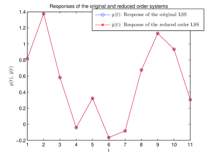
Figure 2: Example $1$: The responses of the original DTLSS $\Sigma$ of order $7$ and the reduced order DTLSS $\bar{\Sigma}$ of order $4$ acquired by Algorithm 3 for the switching sequence in (19).

One more example will be presented to illustrate the case when a representation for the $L$-unobservability space is constructed. The NDFA $\mathcal{A}$ accepting the language of allowed switching sequences is the same one used in the first example; whereas, this time the parameters of the SISO DTLSS $\Sigma$ of order $n=7$ with $Q=\{1,2,3\}$ are in the form:

$$\texttt{A}_{\texttt{1}}=\left[[\texttt{0},\mbox{ }\texttt{1},\mbox{ }\texttt{0},\mbox{ }\texttt{0},\mbox{ }\texttt{0},\mbox{ }\texttt{0},\mbox{ }\texttt{0}];\mbox{ }\texttt{randn(6,7)}\right]$$

$$\texttt{A}_{\texttt{2}}=\left[\texttt{randn(2,7)};\mbox{ }[\texttt{0},\mbox{ }\texttt{0},\mbox{ }\texttt{0},\mbox{ }\texttt{0},\mbox{ }\texttt{0},\mbox{ }\texttt{0},\mbox{ }\texttt{0}];\mbox{ }\texttt{randn(4,7)}\right]$$

$$\texttt{A}_{\texttt{3}}=\left[\texttt{randn(1,7)};\mbox{ }[\texttt{0},\mbox{ }\texttt{0},\mbox{ }\texttt{1},\mbox{ }\texttt{0},\mbox{ }\texttt{0},\mbox{ }\texttt{0},\mbox{ }\texttt{0}];\mbox{ }\texttt{randn(5,7)}\right]$$

$$\texttt{B}_{\texttt{1}}=\texttt{randn(7,1)}$$

$$\texttt{B}_{\texttt{2}}=\texttt{randn(7,1)}$$

$$\texttt{B}_{\texttt{3}}=\texttt{randn(7,1)}$$

$$\texttt{C}_{\texttt{1}}=\texttt{randn(1,7)}$$

$$\texttt{C}_{\texttt{2}}=\left[\texttt{1},\mbox{ }\texttt{0},\mbox{ }\texttt{0},\mbox{ }\texttt{0},\mbox{ }\texttt{0},\mbox{ }\texttt{0},\mbox{ }\texttt{0}\right]$$

$$\texttt{C}_{\texttt{3}}=\texttt{randn(1,7)}$$

Applying Algorithm 3 to this DTLSS, yields a reduced order system $\bar{\Sigma}$ of order $r=3$, whose output values are the same as the original system $\Sigma$ for the instances when the NDFA reaches a final state. Note that this corresponds precisely to an $L$-realization in the sense of Definition 5 (the last outputs of $\Sigma$ and $\bar{\Sigma}$ are the same for all the switching sequences generated by the governing NDFA, i.e., for all $\sigma\in L(\mathcal{A})$). In this example, the algorithm makes use of Lemma 4 and constructs the $W$ matrix. The matrix $W\in\mathbb{R}^{r\times n}$ computed is $W=\left[\begin{array}[]{c|c}I_{3}&\mathbf{0}\end{array}\right]$.

In this example, note that the resulting DTLSS is merely an $L$-realization of $\Sigma$ and nothing more as stated in Remark 3, i.e., its output coincides with the output of $\Sigma$ for only the instances corresponding to the final states of the NDFA. This fact is visible from Figure 3, where it can be seen that output corresponding to the final state $s_{f}$ of the NDFA coincides for $\Sigma$ and $\bar{\Sigma}$ (Observe that for all switching sequences generated by $\mathcal{A}$ ending with the label $2$, the output values of $\Sigma$ and $\bar{\Sigma}$ are the same). Again, the input sequence of length $11$ used in the simulation is generated by the function randn. Finally, note that the DTLSS $\Sigma$ is again minimal whereas for the switching sequences restricted by the NDFA $\mathcal{A}$, it turns out $4$ states are disposable in this case.

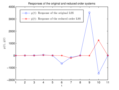
Figure 3: Example $2$: The responses of the original DTLSS $\Sigma$ of order $7$ and the reduced order DTLSS $\bar{\Sigma}$ of order $3$ acquired by Algorithm 3 for the switching sequence in (19). Note that only the second and fifth element of the output sequence is equal for $\Sigma$ and $\bar{\Sigma}$ in first five elements, others look the same as a result of the scaling.

VIII CONCLUSIONS

A model reduction method for discrete time linear switched systems whose discrete dynamics are restricted by switching sequences comprising a regular language is presented. The method is essentially a moment matching type of model reduction method, which focuses on matching the Markov parameters of a DTLSS related to the specific switching sequences generated by a nondeterministic finite state automaton. Possible future research directions include expanding the method for continuous time case, and approximating the input/output behavior of the original system rather than exactly matching it, and formulating the presented algorithms in terms of bisimulation instead of input-output equivalence.

References

- [1] M. Bastug, M. Petreczky, R. Wisniewski, and J. Leth. Model reduction by moment matching for linear switched systems. Proceedings of the American Control Conference, to be published.
- [2] A. Bemporad, G. Ferrari-Trecate, and M. Morari. Observability and controllability of piecewise affine and hybrid systems. IEEE Transactions on Automatic Control, 45(10):1864–1876, 2000.
- [3] A. Birouche, J Guilet, B. Mourillon, and M Basset. Gramian based approach to model order-reduction for discrete-time switched linear systems. In Proc. Mediterranean Conference on Control and Automation, 2010.
- [4] Y. Chahlaoui. Model reduction of hybrid switched systems. In Proceeding of the 4th Conference on Trends in Applied Mathematics in Tunisia, Algeria and Morocco, May 4-8, Kenitra, Morocco, 2009.
- [5] Mircea Lazar Calin Belta Ebru Aydin Gol, Xu Chu Ding. Finite bisimulations for switched linear systems. In IEEE Conference on Decision and Control (CDC) 2012, Maui, Hawaii, 2012.
- [6] Goran Frehse. Phaver: algorithmic verification of hybrid systems past hytech. International Journal on Software Tools for Technology Transfer, 10(3):263–279, 2008.
- [7] H. Gao, J. Lam, and C. Wang. Model simplification for switched hybrid systems. Systems & Control Letters, 55:1015–1021, 2006.
- [8] C.G.J.M. Habets and J. H. van Schuppen. Reduction of affine systems on polytopes. In International Symposium on Mathematical Theory of Networks and Systems, 2002.
- [9] G. Kotsalis, A. Megretski, and M. A. Dahleh. Balanced truncation for a class of stochastic jump linear systems and model reduction of hidden Markov models. IEEE Transactions on Automatic Control, 53(11), 2008.
- [10] G. Kotsalis and A. Rantzer. Balanced truncation for discrete-time Markov jump linear systems. IEEE Transactions on Automatic Control, 55(11), 2010.
- [11] D. Liberzon. Switching in Systems and Control. Birkhäuser, Boston, MA, 2003.
- [12] E. Mazzi, A.S. Vincentelli, A. Balluchi, and A. Bicchi. Hybrid system model reduction. In IEEE International conference on Decision and Control, 2008.
- [13] N. Monshizadeh, H. Trentelman, and M. Camlibel. A simultaneous balanced truncation approach to model reduction of switched linear systems. Automatic Control, IEEE Transactions on, PP(99):1, 2012.
- [14] M. Petreczky. Realization Theory of Hybrid Systems. PhD thesis, Vrije Universiteit, Amsterdam, 2006.
- [15] M. Petreczky. Realization theory for linear and bilinear switched systems: formal power series approach - part i: realization theory of linear switched systems. ESAIM Control, Optimization and Caluculus of Variations, 17:410–445, 2011.
- [16] M. Petreczky, L. Bako, and J. H. van Schuppen. Realization theory of discrete-time linear switched systems. Automatica, 49:3337––3344, November 2013.
- [17] M. Petreczky, R. Wisniewski, and J. Leth. Balanced truncation for linear switched systems. Nonlinear Analysis: Hybrid Systems, 10:4–20, November 2013.
- [18] H.R. Shaker and R. Wisniewski. Generalized gramian framework for model/controller order reduction of switched systems. International Journal of Systems Science, in press, 2011.
- [19] Z. Sun and S. S. Ge. Switched linear systems : control and design. Springer, London, 2005.
- [20] P. Tabuada. Verification and Control of Hybrid Systems: A Symbolic Approach. Springer-Verlag, 2009.
- [21] Arjan van der Schaft and Hans Schumacher. An Introduction to Hybrid Dynamical Systems. Springer-Verlag London, 2000.
- [22] B. Yordanov and C. Belta. Formal analysis of discrete-time piecewise affine systems. Automatic Control, IEEE Transactions on, 55(12):2834–2840, Dec 2010.
- [23] L. Zhang, E. Boukas, and P. Shi. Mu-dependent model reduction for uncertain discrete-time switched linear systems with average dwell time. International Journal of Control, 82(2):378– 388, 2009.
- [24] L. Zhang and P. Shi. Model reduction for switched lpv systems with average dwell time. IEEE Transactions on Automatic Control, 53:2443–2448, 2008.
- [25] L. Zhang, P. Shi, E. Boukas, and C. Wang. Model reduction for uncertain switched linear discrete-time systems. Automatica, 44(11):2944 – 2949, 2008.