The gradient flow running coupling with twisted boundary conditions.

Abstract

We study the gradient flow for Yang-Mills theories with twisted boundary conditions. The perturbative behavior of the energy density $\langle E(t)\rangle$ is used to define a running coupling at a scale given by the linear size of the finite volume box. We compute the non-perturbative running of the pure gauge $SU(2)$ coupling constant and conclude that the technique is well suited for further applications due to the relatively mild cutoff effects of the step scaling function and the high numerical precision that can be achieved in lattice simulations. We also comment on the inclusion of matter fields.

1 Introduction

Non-abelian Yang-Mills theories play a central role in our understanding of high energy physics. Despite their apparent simplicity (they depend on one free parameter, the coupling constant), they have proven to produce very rich phenomena at the quantum level. The invariance under conformal transformations present in the classical theory is broken by quantum corrections and a typical scale of the interactions (usually characterized by the $\Lambda$-parameter) comes into play. The coupling constant becomes scale dependent and asymptotic freedom PhysRevLett.30.1343 ; PhysRevLett.30.1346 guarantees that at high energies its value is small. A perturbative analysis has proven to be very successful in making predictions in this regime, but at low energies the coupling becomes large and non-perturbative effects set in. Confinement characterizes the interaction in this regime and perturbation theory provides little information.

Finite volume renormalization schemes together with non-perturbative numerical simulations Luscher:1991wu ; Luscher:1992an ; deDivitiis:1994yp play a major role in understanding how and when this transition from the perturbative to the non-perturbative regimes of YM theories happens. By identifying the linear size of a finite volume box with the renormalization scale a controlled and non-perturbative running of the coupling constant can be carried over from the very perturbative regime to the non-perturbative one.

There are many practical issues that have made the Schrödinger Functional Luscher:1992an (SF) the preferred scheme to perform the previously mentioned program (see Luscher:1992zx ; Luscher:1993gh ; DellaMorte:2004bc ; Tekin:2010mm for some applications). In the SF one imposes Dirichlet boundary conditions on the spatial components of the gauge fields at $x_{4}=0,T$, while they remain periodic in the spatial directions. By choosing appropriately the values of the fields at the time boundaries one can define a running coupling, usually denoted $g_{\rm SF}^{2}$, with many good properties from a practical point of view. It is easy to evaluate numerically and precise, especially in the perturbative regime.

Other schemes have been proposed: In the twisted Polyakov loop scheme (TPL) the gauge fields are embedded in a torus with twisted boundary conditions and the ratio of Poliakov loops between the twisted and periodic directions is used to define a running coupling deDivitiis:1994yp . This scheme has some good properties, related to the manifest invariance under translations. In particular $\mathcal{O}(a)$ improvement in the pure gauge case is guaranteed, and therefore one expects smaller cutoff effects. On the other hand the observable used to define the coupling tends to be more noisy than the SF coupling.

When one wants to study QCD-like theories, or other models with fermions coupled to the gauge field, similar considerations apply. In the SF scheme Sint:1993un ; Sint:1995rb one can couple an arbitrary number of fermions in any representation to the gauge field. The coupling constant is defined in a similar way, and maintains its good properties. Fermions induce additional boundary counterterms that one needs to compute to have $\mathcal{O}(a^{2})$ scaling. Moreover the boundary conditions for the fermion fields typically break chiral symmetry, and therefore one also needs bulk improvement, although this last issue can be addressed by modifying the boundary conditions of the fermion fields Sint:2010eh . On the other hand, the TPL scheme can not be used with an arbitrary number of fermions in the fundamental representation. The twisted boundary conditions put a constraint on the number of fermions that can be coupled to the gauge field. But when this scheme can be used, it guarantees a better scaling towards the continuum. $\mathcal{O}(a)$ improvement is automatic, even with Wilson fermions, provided that one works with massless quarks Frezzotti:2003ni ; Sint:2010eh . Nevertheless the observable used to define the coupling (a ratio of polyakov loops), tends to be more noisy than the SF coupling, especially in the non-perturbative domain.

Recently the nice properties of the gradient flow regarding the renormalization of composite operators have introduced new observables as candidates for a running coupling definition Luscher:2010iy ; Luscher:2011bx . By introducing an extra parameter (the flow time $t$) one defines a one parameter family of gauge fields. The evolution of the gauge field in flow time is given by a diffusion-like equation that drives the gauge field towards a classical solution of the YM equations, and therefore is a smoothing process. The key point is that the flow field does not require any renormalization at positive flow time ($t>0$), and correlation functions of the smooth field can be considered as observables for a running coupling definition.

In particular the energy density of the flow field

$$\langle E(t)\rangle=\frac{1}{4}\langle G_{\mu\nu}(t)G_{\mu\nu}(t)\rangle\,,$$ (1)

where $G_{\mu\nu}(t)$ is the field strength of the gauge field at flow time $t$, can be used to give a non-perturbative definition of the coupling at a scale $\mu=1/\sqrt{8t}$. Moreover one can identify this renormalization scale with the linear size of the box and define a running coupling.

This idea was first applied to the case of a periodic box Fodor:2012td . The dynamics of Yang-Mills theories in a periodic box contains contributions from zero momentum modes that are not Gaussian and therefore have to be treated exactly GonzalezArroyo:1981vw (see also the review vanBaal:1988qm and references therein). Making a long story short, this leads to a definition of the running coupling that is non-analytic in $g^{2}_{\overline{\rm MS}}$. The author wants to stress that there is nothing wrong with such a coupling definition, but often one wants to make contact with perturbation theory (i.e. when determinning the $\Lambda$ parameter). A non-analytic definition of the coupling may make contact with perturbation theory at a larger energy scale and looses many nice properties, like a universal 2-loop beta function. Moreover perturbative computations in this setup are usually more involved and difficult because one has to treat the zero mode (toron) contribution non perturbatively.

These difficulties can be avoided with a different choice of boundary conditions. For example in the SF, if the boundary values are chosen wisely, zero momentum modes become incompatible with the boundary conditions, and therefore these non Gaussian modes are absent of the dynamics. A definition of a running coupling using the gradient flow in this setup has been proposed in Fritzsch:2013je . It leads to a coupling definition analytic in $g^{2}_{\overline{\rm MS}}$ and with a universal two loop beta function.

The infamous problem of topology freezing that affects large volume simulations Schaefer:2010hu ; Luscher:2011kk , has recently been shown to also affect step scaling studies Fritzsch:2013yxa ; Luscher:2014kea . To overcome this problem it has been proposed Luscher:2014kea to use a setup with mixed boundary conditions. Since in this scheme the fields satisfy open boundary conditions at $x_{0}=T$, topological freezing is avoided Luscher:2012av ; Luscher:2014kea . On the other hand the fields satisfy Dirichlet boundary conditions at $x_{0}=0$, and the absence of zero momentum modes and the analyticity of the observable used to define the coupling is guaranteed.

In this paper we propose another alternative based on using twisted boundary conditions for the gauge fields as in the TPL scheme. These twisted boundary conditions guarantee that the action has a unique minimum up to gauge transformations, and therefore zero momentum modes are not present in the dynamics. Moreover the formulation is manifestly translation invariant, since the scheme is defined in a torus, guaranteeing the absence of $\mathcal{O}(a)$ effects, even when one works with massless Wilson fermions.

This paper is organized as follows. Section 2 presents a small review of the twisted boundary conditions. Readers interested in more details are encouraged to look at the review ga:torus and the recent paper Perez:2013dra . Section 3 studies the perturbative behavior of the gradient flow with twisted boundary conditions. Again we encourage the reader to consult the original works Luscher:2010iy ; Luscher:2011bx for a better understanding of the properties of the gradient flow. Section 4 uses the previous results to define a non-perturbative coupling that runs with the size of the box. Finally in section 5 we compute the running coupling for the case of an $SU(2)$ pure gauge theory, and conclude that the modest size of cutoff effects and small variance of the observable when using Monte Carlo techniques to compute it, make it an interesting choice for further studies.

2 Twisted boundary conditions

The twisted boundary conditions were first introduced by ’t Hooft tHooft:1979uj to characterize confinement. But for us, they will be used simply as a tool to study the renormalization of Yang-Mills theories. The main observation is that the requirement for physical quantities to be periodic can be accomplished by fields that change by a gauge transformation under translations over a period.

2.1 Gauge fields

We will consider $SU(N)$ gauge fields in a four dimensional torus of size $L^{4}$. The twisted boundary conditions are implemented by requiring the field to gauge-transform under the displacement of a period

$$A_{\mu}(x+L\hat{\nu})=\Omega_{\nu}(x)A_{\mu}(x)\Omega_{\nu}^{+}(x)+\Omega_{\nu}(x)\partial_{\mu}\Omega_{\nu}^{+}(x)\,,$$ (2)

where $\Omega_{\mu}(x)$ are known as the twist matrices. The uniqueness of $A_{\mu}(x+L\hat{\mu}+L\hat{\nu})$ requires that the twist matrices have to obey the relation

$$\Omega_{\mu}(x+L\hat{\nu})\Omega_{\nu}(x)=e^{2\pi\imath n_{\mu\nu}/N}\Omega_{\nu}(x+L\hat{\mu})\Omega_{\mu}(x)\,,$$ (3)

where $n_{\mu\nu}$ is an anti-symmetric tensor of integers modulo $N$ called the twist tensor. It is easy to check that under a gauge transformation, $\Lambda(x)$, the twist matrices change according to

$$\Omega_{\nu}(x)\longrightarrow\Omega^{\prime}_{\nu}(x)=\Lambda(x+L\hat{\nu})\Omega_{\nu}(x)\Lambda^{+}(x)\,,$$ (4)

but the twist tensor $n_{\mu\nu}$ remains unchanged. Therefore all the physics of the twisted boundary conditions is contained in the twist tensor, and the particular choice of twist matrices is irrelevant. One can restrict the gauge transformations to those that leave the twist matrices unchanged. It is easy to check that the necessary and sufficient condition for the gauge transformations is to obey the periodicity condition

$$\Lambda(x+L\hat{\nu})=\Omega_{\nu}(x)\Lambda(x)\Omega_{\nu}^{+}(x)\,.$$ (5)

The reader interested in knowing more about the twisted boundary conditions is invited to consult the review ga:torus . Here we will use a particular setup: we choose to twist only one plane (the $x_{1}-x_{2}$ plane) by choosing $n_{12}=-n_{21}=1$, while the rest of the components of the twist tensor will be zero. This means that our gauge connections will still be periodic in the $x_{3}$ and $x_{4}$ directions. As we will see, this choice guarantees that the action has a unique minimum (modulo gauge transformations), and therefore it turns out to be a convenient choice for perturbative studies. This is the reason why the very same choice has been made before to define the Twisted Polyakov Loop running coupling scheme deDivitiis:1994yp , or for other perturbative studies Luscher:1985wf . We will closely follow the notation and steps presented in Perez:2013dra , a reference that the reader interested in more details should consult.

A convenient implementation of twisted boundary conditions consists in using space-time independent twist matrices. In particular for the periodic directions we set the twist matrices to one

$$\Omega_{1,2}(x) = \Omega_{1,2}$$ (6a)

$$\Omega_{3,4}(x) = 1\,.$$ (6b)

We will use latin indexes ($i,j,\dots=1,2$) to run over the directions in the twisted plane, while greek indexes ($\mu,\nu,\dots=0,\dots,3$) will run over the four space time directions. The consistency relation Eq. (3) implies the following condition for the twist matrices

$$\Omega_{1}\Omega_{2}=e^{2\pi\imath/N}\Omega_{2}\Omega_{1}.$$ (7)

Notice that the boundary conditions for the gauge field with this choice of the twist matrices are

$$A_{\mu}(x+L\hat{k})=\Omega_{k}A_{\mu}(x)\Omega_{k}^{+}\,,$$ (8)

and $A_{\mu}=0$ is a valid connection. In fact we will show that it is the only connection compatible with the boundary conditions that does not depend on $x$, and therefore it is the unique minimum of the action modulo gauge transformations.

Eq. (8) defines a generalization of the Dirac algebra. It can be shown ga:torus that there is a unique solution for the matrices $\Omega_{i}$ modulo similarity transformations. Introducing the color momentum, $\tilde{p}_{i}=\frac{2\pi\tilde{n}_{i}}{NL}$ with $n_{i}=0,\dots,N-1$ it is easy to check that the $N^{2}$ matrices

$$\Gamma(\tilde{p})=\frac{\imath}{\sqrt{2N}}e^{\imath\alpha(\tilde{p})}\Omega_{1}^{-\tilde{n}_{2}}\Omega_{2}^{\tilde{n}_{1}}\,,$$ (9)

where $\alpha(\tilde{p})$ are arbitrary phases, are linearly independent and obey the relation

$$\Omega_{i}\Gamma(\tilde{p})\Omega_{i}^{+}=e^{\imath L\tilde{p}_{i}}\Gamma(\tilde{p})\,.$$ (10)

Moreover all but $\Gamma(\tilde{p}=0)$ are traceless, and therefore they can be used as a basis of the Lie algebra of the gauge group. This means that any gauge connection can be expanded as

$$A_{\mu}^{a}(x)T^{a}=\sum_{\tilde{p}}^{\prime}\hat{A}_{\mu}(x,\tilde{p})e^{\imath\tilde{p}x}\Gamma(\tilde{p}).$$ (11)

The prime over the sum means that the term $\tilde{p}_{i}=0$ is absent in the sum, as required for a $SU(N)$ gauge group. Notice that the coefficients $\hat{A}_{\mu}(x,\tilde{p})$ are functions (not matrices) periodic in $x$. Therefore one can do an usual Fourier expansion and obtain

$$A_{\mu}^{a}(x)T^{a}=\frac{1}{L^{4}}\sum_{p,\tilde{p}}^{\prime}\tilde{A}_{\mu}(p,\tilde{p})e^{\imath(p+\tilde{p})x}\Gamma(\tilde{p})\,,$$ (12)

with the usual spatial momentum

$$p_{\mu}=\frac{2\pi n_{\mu}}{L}\quad(n_{\mu}\in\mathbb{Z})\,.$$ (13)

Finally we define the total momentum as the sum of the color and space momentum $P_{i}=p_{i}+\tilde{p}_{i}$, $P_{3,4}=p_{3,4}$. Noting that any $P_{\mu}$ can be uniquely decomposed in the space momentum and color momentum degrees of freedom we can safely write $\Gamma(P)$ instead of $\Gamma(\tilde{p})$. Our main conclusion is that any gauge connection compatible with our choice of boundary conditions can be written as

$$A_{\mu}^{a}(x)T^{a}=\frac{1}{L^{4}}\sum_{P}^{\prime}\tilde{A}_{\mu}(P)e^{\imath Px}\Gamma(P)\,.$$ (14)

In particular the only connection that does not depend on $x$ is given by $\tilde{A}_{\mu}(P)=0$. In general the matrices $\Gamma(P)$ are not anti-hermitian, but one can choose the phases $\alpha(P)$ of equation (9) so that this condition is enforced

$$\alpha(P)=\frac{\theta}{2}P_{1}P_{2}\qquad\left(\theta=\frac{NL^{2}}{2\pi}\right)\,.$$ (15)

In this case, the Fourier coefficients $\tilde{A}_{\mu}(P)$ satisfy the usual relation

$$\tilde{A}_{\mu}(P)^{*}=\tilde{A}_{\mu}(-P)\,,$$ (16)

and the $\Gamma$ matrices are normalized according to

$${\rm Tr}\left\{\Gamma(P)\Gamma(-P)\right\}=-\frac{1}{2}\,.$$ (17)

We finally note that a simlar expansion is possible on the lattice, with the only difference that the space momentum will be restricted to the Brillouin zone.

2.2 Matter fields

The inclusion of matter fields interacting with gauge fields with twisted boundary conditions is not completely straightforward. To understand why it is better first to consider how to include fermion fields in the fundamental representation. Since the twist matrices tell us how fields change under translations, one naively expects

$$\psi(x+L\hat{i})=\Omega_{i}\psi(x)\,,$$ (18)

but one can easily see that this choice is not consistent, since the value of the field $\psi(x+L\hat{i}+L\hat{j})$ depends on the order in which we perform the translations due to the non-commutativity of the twist matrices. This difficulty can be avoided by introducing more fermions, or what usually is called a “smell” degree of freedom Parisi:1984cy . If $\alpha,\beta=1,\dots,N_{s}$ are indices that run over the $N_{s}$ smells of fermions, and $a,b=1,\dots,N$ run over the color degrees of freedom, the boundary conditions of the fermions read

$$\psi^{a}_{\alpha}(x+L\hat{i})=e^{\imath\theta_{i}}(\Omega_{i})_{ab}(\Omega^{*}_{i})_{\alpha\beta}\psi^{b}_{\beta}(x)\,.$$ (19)

This means that a fermion smell becomes a linear combination of the gauge transformed fermion smells under a translation. $\theta_{i}$ are in principle arbitrary, but introduced for convenience to remove the zero-momentum modes of the Dirac operator. These phases have to be chosen such that they are not elements of the gauge group (i.e. $e^{\imath\theta}\not\in SU(N)$). This choice of boundary conditions for the fermion fields is consistent, but they require the number of smells to be equal to the number of colors. One can easily extend the construction to the case when the ratio $N_{s}/N$ is an integer, but in general one can not have an arbitrary number of fermions in the fundamental representation.

On the other hand fermions in the adjoint representation transform in the same way as the gauge fields, and therefore any number of fermions would be compatible with the twisted boundary conditions.

Regardless of the representation but assuming that the matter fields are compatible with the twisted boundary conditions, $\mathcal{O}(a)$ improvement for massless Wilson quarks is automatically satisfied since fields live on a torus, and the boundary conditions do not break chiral symmetry (see Sint:2010eh ; Frezzotti:2003ni ).

3 The gradient flow in a twisted box

The gradient flow has recently proved to be an interesting tool to study several aspects of YM theories Narayanan:2006rf ; Luscher:2009eq ; Luscher:2010iy ; Luscher:2011bx ; Luscher:2013cpa . By introducing an extra coordinate $t$, called flow time (not to be confused with Euclidean time $x_{0}$), gauge fields are smoothed along the flow according to the equation

$$\frac{{\rm d}B_{\mu}(x,t)}{{\rm d}t} = D_{\nu}G_{\nu\mu}$$ (20a)

$$B(x,0) = A_{\mu}(x)$$ (20b)

where $D_{\mu}=\partial_{\mu}+B_{\mu}$ is the covariant derivative and $G_{\mu\nu}=\partial_{\mu}B_{\nu}-\partial_{\nu}B_{\mu}+[B_{\mu},B_{\nu}]$ is the field strength tensor. The main reason why renormalization problems are highly simplified with the use of the gradient flow is that correlations functions made of the flow field $B_{\mu}(x,t)$ do not need renormalization at positive flow time Luscher:2011bx . In particular the energy density

$$\langle E(t)\rangle=-\frac{1}{2}\langle{\rm Tr}\left\{G_{\mu\nu}(x,t)G_{\mu\nu}(x,t)\right\}\rangle$$ (21)

is a renormalized quantity at a scale $\mu=1/\sqrt{8t}$ and can be used (at $t>0$) to define a renormalized coupling Luscher:2010iy . Moreover one can use a finite box to define a finite volume renormalization scheme by running the renormalization scale with the linear size of a finite volume box Fodor:2012td ; Fritzsch:2013je ; Luscher:2014kea

$$\mu=\frac{1}{\sqrt{8t}}=\frac{1}{cL}\,.$$ (22)

The constant $c$ parametrizes the ratio between the renormalization scale and the linear size of the box $L$, and is part of the definition of the renormalization scheme.

Being a finite volume renormalization scheme, the boundary conditions are relevant. The idea has been applied in a four dimensional torus with periodic boundary conditions Fodor:2012td , with Schrödinger functional boundary conditions Fritzsch:2013je , and also with mixed boundary conditions Luscher:2014kea . In this work we will give a definition of a running coupling in a four dimensional torus with twisted boundary conditions, but first we need to study the perturbative behavior of $\langle E(t)\rangle$ in a twisted box.

3.1 Perturbative behavior of the gradient flow in a twisted box: continuum

3.1.1 Generalities and gauge fixing

We are interested in the perturbative expression for $\langle E(t)\rangle$, and in order to avoid some difficulties in the definition of propagators, it turns out to be convenient to fix the gauge of the flow field $B_{\mu}(x,t)$. This can be achieved by studying the modified flow equation

$$\frac{{\rm d}B_{\mu}^{(\alpha)}(x,t)}{{\rm d}t}=D_{\nu}^{(\alpha)}G_{\nu\mu}^{(\alpha)}(x,t)+\alpha D_{\mu}^{(\alpha)}\partial_{\nu}B_{\nu}^{(\alpha)}(x,t)\,.$$ (23)

The superscript ${(\alpha)}$ recalls that covariant derivatives and field strength are made of the modified flow field $B_{\mu}^{(\alpha)}(x,t)$, solution of the previous equation. A solution of this modified flow equation $B_{\mu}^{(\alpha)}(x,t)$ can be transformed in a solution of the original flow equation (20b) by a time dependent gauge transformation Luscher:2011bx

$$B_{\mu}=\Lambda B_{\mu}^{(\alpha)}\Lambda^{-1}+\Lambda\partial_{\mu}\Lambda^{-1}\,,$$ (24)

where

$$\frac{{\rm d}\Lambda}{{\rm d}t}=\alpha\Lambda\partial_{\mu}B_{\mu}\,;\quad\Lambda\big{|}_{t=0}=1\,.$$ (25)

Therefore gauge invariant quantities are independent of $\alpha$. Note that the previously defined gauge transformation $\Lambda(x)$ belongs to the restricted set of gauge transformations that leave the twist matrices invariant (see equation (5)), and the boundary conditions of $B_{\mu}^{(\alpha)}$ are also independent of $\alpha$.

3.1.2 Flow field and energy density to leading order

The particular choice $\alpha=1$ simplify the computations, and we will use it for the rest of this section. The modified flow equation reads in this case

$$\frac{{\rm d}B_{\mu}}{{\rm d}t}=D_{\nu}G_{\nu\mu}+D_{\mu}\partial_{\nu}B_{\nu}\,.$$ (26)

In perturbation theory one re-scales the gauge potential with the bare coupling $A_{\mu}\rightarrow g_{0}A_{\mu}$, and the flow field has an asymptotic expansion in the bare coupling

$$B_{\mu}(x,t)=\sum_{n=1}^{\infty}B_{\mu,n}(x,t)g_{0}^{n}\,.$$ (27)

To leading order our flow equation (26) is just the heat equation

$$\frac{{\rm d}B_{\mu,1}(x,t)}{{\rm d}t} = \partial_{\nu}^{2}B_{\mu,1}(x,t)$$ (28)

$$B_{\mu,1}(x,0) = A_{\mu}(x)\,,$$ (29)

expanding $B_{\mu,1}(x,t)$ in our preferred basis (14) one can easily solve (28) and obtain

$$B_{\mu,1}(x,t)=\frac{1}{L^{4}}\sum_{P}^{\prime}e^{-P^{2}t}\tilde{A}_{\mu}(P)e^{\imath Px}\Gamma(P)\,.$$ (30)

Finally our observable of interest also has an expansion in powers of $g_{0}$

$$\langle E(t)\rangle=-\frac{1}{2}\langle{\rm Tr}\{G_{\mu\nu}(x,t)G_{\mu\nu}(x,t)\}\rangle=\mathcal{E}(t)+\mathcal{O}(g_{0}^{4})\,.$$ (31)

One can easily obtain

$$\mathcal{E}(t) = \frac{g_{0}^{2}}{2}\langle\partial_{\mu}B_{\nu,1}\partial_{\mu}B_{\nu,1}-\partial_{\mu}B_{\nu,1}\partial_{\nu}B_{\mu,1}\rangle$$

$$= \frac{-g_{0}}{2L^{8}}\sum_{P,Q}^{\prime}e^{-(P^{2}+Q^{2})t}e^{\imath(P+Q)x}\left(P_{\alpha}Q_{\alpha}\delta_{\mu\nu}-P_{\mu}Q_{\nu}\right)\langle\tilde{A}_{\mu}(P)\tilde{A}_{\nu}(Q)\rangle{\rm Tr}(\hat{\Gamma}(P)\hat{\Gamma}(Q))\,.$$

Finally using the expression for the gluon propagator

$$\langle\tilde{A}_{\mu}(P)\tilde{A}_{\nu}(Q)\rangle=L^{4}\delta_{P_{\alpha},-Q_{\alpha}}\frac{1}{P^{2}}\left[\delta_{\mu\nu}-(1-\lambda^{-1})\frac{P_{\mu}P_{\nu}}{P^{2}}\right]\frac{1}{{\rm Tr}({\Gamma(-P)\Gamma(P)})}+\mathcal{O}(g_{0}^{2})$$ (33)

one gets

$$\mathcal{E}(t)=\frac{3g_{0}^{2}}{2L^{4}}\sum_{P}^{\prime}e^{-2P^{2}t}\,.$$ (34)

3.2 Perturbative behavior of the gradient flow in a twisted box: lattice

When defining the gradient flow in the lattice one has to make several choices. These basically correspond to the particular discretizations of the action whose gradient is used to define the flow, as well as the discretization of the energy density and the choice of action that one simulates (i.e. Wilson/improved actions).

First we will analyze the popular case where the Wilson action is simulated, and one uses the same action to define the flow (in this case is called the Wilson flow). The clover definition of the observable has been a typical choice Luscher:2010iy for a discretization of the energy density. Later we will comment on the general case.

3.2.1 Generalities and gauge fixing

On the lattice the gradient flow is substituted by a discretized version. There are several possibilities: one can use the Wilson action

$$S_{w}(V)=\frac{1}{g_{0}^{2}}\sum_{\rm p}{\rm Re}\{{\rm Tr}(1-U_{\rm p})\}$$ (35)

where the sum runs over the oriented plaquettes, and define the flow equation by equating the time derivative of the links with the gradient of the Wilson action

$$a^{2}\partial_{t}V_{\mu}(x,t)=-g_{0}^{2}\{T^{a}\partial_{x,\mu}^{a}S_{w}(V)\}V_{\mu}(x,t)\,,\qquad V_{\mu}(x,0)=U_{\mu}(x)\,.$$ (36)

In this case the gradient flow is usually referred as the Wilson flow. Some explanations of our notation are in order. If $f(U_{\mu}(x))$ is an arbitrary function of the link variable $U_{\mu}(x)$, the components of its Lie-algebra valued derivative $\partial_{x,\mu}^{a}$ are defined as

$$\partial_{x,\mu}^{a}f(U_{\mu}(x))=\left.\frac{{\rm d}f(e^{\epsilon T^{a}}U_{\mu}(x))}{{\rm d}\epsilon}\right|_{\epsilon=0}\,.$$ (37)

In perturbation theory one is interested in a neighborhood of the classical vacuum configuration. In this neighborhood the lattice fields $U_{\mu}(x)$ and $V_{\mu}(x,t)$ are parametrized as follows:

$$U_{\mu}(x) =\exp\{ag_{0}A_{\mu}(x)\}\;, V_{\mu}(x,t) =\exp\{ag_{0}B_{\mu}(x,t)\}\;.$$ (38)

Again it is convenient to study a modified flow equation where the gauge degrees of freedom are damped. We will consider

$$a^{2}\partial_{t}V_{\mu}^{\Lambda}(x,t)=g_{0}^{2}\left\{-\big{[}T^{a}\partial_{x,\mu}^{a}S_{w}(V^{\Lambda})\big{]}+a^{2}\hat{D}_{\mu}^{\Lambda}\big{[}\Lambda^{-1}(x,t)\dot{\Lambda}(x,t)\big{]}\right\}V_{\mu}^{\Lambda}(x,t)\,,$$ (39)

with $V_{\mu}^{\Lambda}(x,0)=U_{\mu}(x)$ and the forward lattice covariant derivative $\hat{D}_{\mu}^{\Lambda}$ acting on Lie-algebra valued functions according to

$$\hat{D}_{\mu}f(x)=\frac{1}{a}\left[V_{\mu}(x,t)f(x+\hat{\mu})V_{\mu}^{-1}(x,t)-f(x)\right]\,.$$ (40)

Solutions of the modified and original flow equations are related by a gauge transformation

$$V_{\mu}(x,t)=\Lambda(x,t)V_{\mu}^{\Lambda}(x,t)\Lambda^{-1}(x+\hat{\mu},t)\,.$$ (41)

The most natural choice for $\Lambda(x,t)$ is the same functional used for gauge fixing

$$\Lambda^{-1}\frac{{\rm d}\Lambda}{{\rm d}t}=\alpha\hat{\partial}^{*}_{\mu}B_{\mu}(x,t)\,,\qquad\Lambda\big{|}_{t=0}=1\,.$$ (42)

where $\hat{\partial},\hat{\partial}^{*}$ denote the forward/backward finite differences. We again note that the boundary conditions of $V_{\mu}^{\Lambda}(x,t)$ are independent of $\alpha$, since $\Lambda(x,t)$ belongs to the restricted class of gauge transformations that leave the twist matrices unchanged.

3.2.2 Flow field and energy density to leading order

Again the choice $\alpha=1$ turns out to be convenient and we will stick to it from now on.

The modified flow equation reads

$$a^{2}\partial_{t}V_{\mu}(x,t)=g_{0}^{2}\left\{-[T^{a}\partial_{x,\mu}^{a}S_{w}(V)]+a^{2}\hat{D}_{\mu}(\hat{\partial}_{\nu}^{*}B_{\nu})\right\}V_{\mu}(x,t)\,,\qquad V_{\mu}(x,0)=U_{\mu}(x)\,.$$ (43)

The flow field can be expanded in powers of $g_{0}$ (equation (27)) and to first order in $g_{0}$ we have

$$\partial_{t}B_{\mu,1}(x,t)=\hat{\partial}_{\nu}\hat{\partial}_{\nu}^{*}B_{\mu,1}(x,t)\,.$$ (44)

Expanding the flow field in our favorite Lie-algebra basis (equation (14)) one can write the solution to the previous equation

$$B_{\mu,1}(x,t)=\frac{1}{L^{4}}\sum_{P}^{\prime}e^{-\hat{P}^{2}t}\tilde{A}_{\mu}(P)e^{\imath Px}\Gamma(P)\,,$$ (45)

where

$$\hat{P}_{\mu}=\frac{2}{a}\sin\left(a\frac{P_{\mu}}{2}\right)$$ (46)

is the usual lattice momentum.

We can choose among different discretizations for the energy density. The most popular one consists in using the clover definition for $G_{\mu\nu}(x,t)$ Luscher:2010iy . To leading order we have

$$\hat{G}_{\mu\nu}(x,t) = \frac{g_{0}}{2}\,\mathring{\partial}_{\mu}\left[B_{\nu,1}(x,t)+B_{\nu,1}(x-\hat{\nu},t)\right]$$ (47)

$$- \frac{g_{0}}{2}\,\mathring{\partial}_{\nu}\left[B_{\mu,1}(x,t)+B_{\mu,1}(x-\hat{\mu},t)\right]+\mathcal{O}(g_{0}^{2})\,,$$

where $\mathring{\partial}_{\mu}=\tfrac{1}{2}(\hat{\partial}_{\mu}+\hat{\partial}^{*}_{\mu})$ is the symmetric finite difference. The energy density computed with the clover definition for the field strength tensor reads

$$\langle E^{\rm cl}(t)\rangle=-\frac{1}{2}\langle{\rm Tr}\{\hat{G}_{\mu\nu}\hat{G}_{\mu\nu}\}\rangle=\mathcal{E}^{\rm cl}(t,a/L)+\mathcal{O}(g_{0}^{2})$$ (48)

Using the definitions

$$\mathring{P}_{\mu} = \frac{1}{a}\sin\left(aP_{\mu}\right)\,,$$ (49a)

$$C_{\mu} = \cos\left(a\frac{P_{\mu}}{2}\right)\,,$$ (49b)

and the lattice gluon propagator, one can easily obtain

$$\hat{\mathcal{E}}^{\rm cl}(t,a/L)=\frac{g_{0}^{2}}{2L^{4}}\sum_{P}^{\prime}e^{-2\hat{P}^{2}t}\frac{\mathring{P}^{2}C^{2}-(\mathring{P}_{\mu}C_{\mu})^{2}}{\hat{P}^{2}}\,.$$ (50)

3.2.3 Some comments on different discretizations

In general the lattice computation of the leading order behavior of the energy density involves several choices of discretization: the action that one simulates (labelled (a)), the action whose gradient defines the flow evolution (labelled (f)), and finally the discretization used to compute the observable (labelled (O)). To leading order, these three choices can be expressed as choice of “actions”

$$S_{a}[\tilde{A}_{\mu}] = \frac{1}{4L^{4}}\sum_{P}^{\prime}\tilde{A}_{\mu}(-P)K_{\mu\nu}^{(a)}(P)\tilde{A}_{\nu}(P)+\mathcal{O}(g_{0}^{2})\,,$$ (51a)

$$S_{f}[\tilde{A}_{\mu}] = \frac{1}{4L^{4}}\sum_{P}^{\prime}\tilde{A}_{\mu}(-P)K_{\mu\nu}^{(f)}(P)\tilde{A}_{\nu}(P)+\mathcal{O}(g_{0}^{2})\,,$$ (51b)

$$S_{O}[\tilde{A}_{\mu}] = \frac{1}{4L^{4}}\sum_{P}^{\prime}\tilde{A}_{\mu}(-P)K_{\mu\nu}^{(O)}(P)\tilde{A}_{\nu}(P)+\mathcal{O}(g_{0}^{2})\,.$$ (51c)

The matrices $K^{(a)}$ and $K^{(f)}$ may (and should) contain a gauge fixing part, but not the one corresponding to the observable $K^{(O)}$. In this way final results will be independent of the choices of gauge. The inverse of the $K_{\mu\nu}^{(a)}$ defines the lattice gluon propagator

$$\langle A_{\mu}(-P)A_{\nu}(P)\rangle = D_{\mu\nu}(P)\,,$$ (52)

$$K_{\mu\alpha}^{(a)}(P)D_{\alpha\nu}(P) = \delta_{\mu\nu}\,.$$ (53)

Using this notation it is trivial to obtain the form of the flow field to leading order

$$\tilde{B}_{\mu,1}(P)=\left(\exp\{-tK^{(f)}(P)\}\right)_{\mu\nu}\tilde{A}_{\nu}(P)=H_{\mu\nu}(t,P)\tilde{A}_{\nu}(P)\,,$$ (54)

and noting that the reality of the action requires that $H^{+}(t,P)=H(t,-P)$, we can write the expression of the energy density to leading order as

$$\mathcal{E}(t,a/L) = g_{0}^{2}\langle S_{O}[\tilde{B}_{\mu,1}]\rangle$$ (55)

$$= \frac{g_{0}^{2}}{2L^{4}}\sum_{P}^{\prime}{\rm Tr}\{H^{+}(t,P)K^{(O)}(P)H(t,P)D(P)\}\,.$$ (56)

This formula allows an easy evaluation of the energy density, to leading order in perturbation theory, for any choice of discretizations. One general point that one can make is that if one uses the Wilson flow the matrix $H(t,P)$ can be chosen to be proportional to the identity (by an appropriate gauge choice), and therefore commutes with any other matrix. Moreover if the action that one simulates is the same as the one that we use to compute the observable, the product of matrices $DK^{O}$ together with the trace simply result in a factor 3, and therefore one obtains

$$\mathcal{E}(t,a/L)=\frac{3g_{0}^{2}}{2L^{4}}\sum_{P}^{\prime}e^{-2t\hat{P}^{2}}\,.$$ (57)

This means that without changing the flow, improving the action and the observable leads to exactly the same cutoff effects than if one does not improve anything (to leading order).

3.3 Tests

In order to check the previous computations one can perform several consistency checks. First it is obvious that the continuum result (equation (34)) is recovered from the lattice one (equation (50)) if one takes the limit $a/L\rightarrow 0$. In the infinite volume limit boundary conditions are irrelevant, and therefore for $L\rightarrow\infty$ one should recover the result of Luscher:2010iy that reads

$$\mathcal{E}^{(L=\infty)}(t)=\frac{3g_{0}^{2}(N^{2}-1)}{128\pi^{2}t^{2}}\,.$$ (58)

This result is reproduced from our expression equation (34) by simply noting that

$$P_{\mu}=\frac{2\pi}{L}\left(n_{\mu}+\frac{\tilde{n}_{\mu}}{N}\right)\,,$$ (59)

and therefore

$$\frac{1}{L^{4}}\sum_{P}^{\prime}\xrightarrow[L\rightarrow\infty]{}\frac{1}{(2\pi)^{4}}\sum_{\tilde{p}_{i}}^{\prime}\int_{-\infty}^{\infty}{\rm d}^{4}P\,.$$ (60)

Finally recalling that there are $N^{2}-1$ terms in the sum over $\tilde{p}_{i}$ (the term $\tilde{p}_{i}=0$ is explicitly excluded) one obtains

$$\mathcal{E}(t)\xrightarrow[L\rightarrow\infty]{}\frac{3g_{0}^{2}}{32\pi^{4}}\sum_{\tilde{p}_{i}}^{\prime}\int_{-\infty}^{\infty}{\rm d}^{4}Pe^{-2P^{2}t}=\frac{3g_{0}^{2}(N^{2}-1)}{128\pi^{2}t^{2}}\,.$$ (61)

To check the lattice computations we have performed some dedicated pure gauge lattice simulations. We use the plaquette action of an $SU(2)$ gauge theory in two different volumes $L/a=4^{4}$ and $L/a=6^{4}$. We collect $10,000$ measurements of $\langle E^{\rm cl}(t)\rangle$ for different values of $t$ and $\beta=2/g_{0}^{2}=40,80,120,200,400,560,800,960,1120,1280$. In these large-$\beta$ simulations the measured $\langle E^{\rm cl}(t)\rangle$ should reproduce the perturbative expression (equation (50)). Being more precise, we will study numerically the quantity

$$R(g_{0},t)=\frac{\langle E^{\rm cl}(t)\rangle-\mathcal{E}^{\rm cl}(t)}{\mathcal{E}^{\rm cl}(t)}\,.$$ (62)

We expect that $R(g_{0},t)=\mathcal{O}(g_{0}^{2})$, and therefore by fitting the data from the simulations to a linear behavior

$$R(g_{0},t)=m(t)g_{0}^{2}+n(t)$$ (63)

one should obtain an intercept $n(t)$ compatible with zero within errors. Indeed this is the case, for different values of $t$ and $L$, as the reader can check in table (1). A couple of representative fits are shown in the figure 1.

$V$		$c$
		0.30	0.35	0.40	0.45	0.50
$4^{4}$	$\chi^{2}/{\rm ndof}$	1.4	1.5	1.6	1.7	1.7
	$\mathcal{E}(t,a/L)$	$1.37\times 10^{-1}$	$9.76\times 10^{-2}$	$6.58\times 10^{-2}$	$3.22\times 10^{-2}$	$2.53\times 10^{-2}$
	$n\times 10^{4}$	$2.5(4.7)$	$3.4(6.2)$	$4.8(8.1)$	$6.8(10)$	$9.5(12)$
$6^{4}$	$\chi^{2}/{\rm ndof}$	0.34	0.44	0.62	0.83	1.03
	$\mathcal{E}(t,a/L)$	$3.78\times 10^{-2}$	$2.20\times 10^{-2}$	$1.39\times 10^{-2}$	$7.82\times 10^{-3}$	$5.45\times 10^{-3}$
	$n\times 10^{4}$	$-1.8(1.6)$	$-3.1(2.5)$	$-4.5(3.9)$	$-6.0(5.9)$	$-7.4(8.2)$

Table 1: Results of a linear fit of $R(g_{0},t)$ for different lattice sizes and different flow times $t$. In the table the flow time is parametrized by $c=\frac{\sqrt{8t}}{L}$. As one can observe all fits have a good fit quality and the intercept of the fit (given by $n$) is compatible with zero within errors.

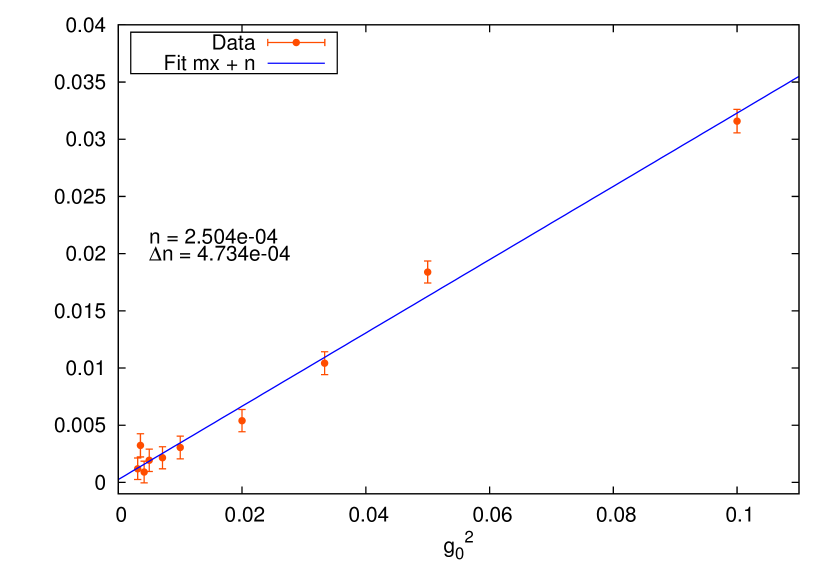
(a) Fit for $L=4^{4}$ and $c=0.3$.

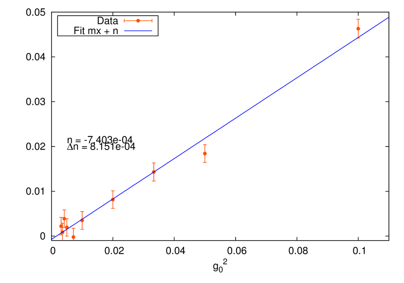
(b) Fit for $L=6^{4}$ and $c=0.5$

Figure 1: Some representative fits to the large-$\beta$ simulations. The plots show the function $R(g_{0},t)$ at fixed $t=c^{2}L^{2}/8$ versus $g_{0}^{2}$.

4 Running coupling definition

The computations of the previous section guarantee that

$$t^{2}\langle E(t)\rangle=g_{0}^{2}\left[\frac{3t^{2}}{2L^{4}}\sum_{P}^{\prime}e^{-2P^{2}t}\right]+\mathcal{O}(g_{0}^{4})\,.$$ (64)

On the other hand the properties of the gradient flow ensures that $t^{2}\langle E(t)\rangle$ is a renormalized observable defined at a scale $\mu=1/\sqrt{8t}$. This suggests that one can use $t^{2}\langle E(t)\rangle$ for a non-perturbative coupling definition. Moreover if one keeps the product of the renormalization scale and the linear size of the box fixed (i.e. $\mu L=1/c={\rm constant}$) the coupling will depend on no scale other than the linear size of the box, and therefore will be ideal for finite size scaling.

In full glory our coupling definition reads

$$g_{\rm TGF}^{2}(L)=\mathcal{N}^{-1}_{T}(c)t^{2}\langle E(t)\rangle\Big{|}_{t=c^{2}L^{2}/8}$$ (65)

where

$$\mathcal{N}_{T}(c)=\frac{3c^{4}}{128}\sum_{P}^{\prime}e^{-\frac{c^{2}L^{2}}{4}P^{2}}=\frac{3c^{4}}{128}\sum_{n_{\mu}=-\infty}^{\infty}{\sum_{\tilde{n}_{i}=0}^{N-1}}^{\prime}e^{-{\pi^{2}c^{2}}(n^{2}+\tilde{n}^{2}/N^{2}+2\tilde{n}_{i}n_{i}/N)}\,.$$ (66)

This coupling has a perturbative expansion

$$g_{\rm TGF}^{2}(L)=g_{\rm\overline{MS}}^{2}+\mathcal{O}(g_{\rm\overline{MS}}^{4})$$ (67)

and a universal two loop $\beta$-function

$$L\frac{\partial g_{\rm TGF}^{2}}{\partial L}=-\frac{\beta_{0}}{16\pi^{2}}g_{\rm TGF}^{4}-\frac{\beta_{1}}{\left(16\pi^{2}\right)^{2}}g_{\rm TGF}^{6}+\mathcal{O}(g_{\rm TGF}^{8})$$ (68)

where the universal coefficients, for the case of an $SU(N)$ YM theory are given by

$$\beta_{0}=\frac{11N}{3}\,,\qquad\beta_{1}=\frac{34N^{2}}{3}\,.$$ (69)

We point out that the same coupling definition is valid if one includes any number of fermions in any representation, as soon as they are allowed by the twisted boundary conditions (more details in section 2.2).

4.1 Cutoff effects in the twisted running coupling

The comparison of the lattice and the continuum computations of $\mathcal{E}(t)$ can give us an idea of the size of cutoff effects (to leading order in $g_{0}^{2}$) of the twisted gradient flow coupling. We are going to study in detail the case of lattice simulations using the Wilson action, the Wilson flow, and the clover definition for the observable. If we define

$$\hat{\mathcal{N}}_{T}(c,a/L)=\frac{c^{4}}{128}\sum_{P}^{\prime}e^{-\frac{c^{2}L^{2}}{4}\hat{P}^{2}}\frac{\mathring{P}^{2}C^{2}-(\mathring{P}_{\mu}C_{\mu})^{2}}{\hat{P}^{2}}\,,$$ (70)

the quantity

$$Q(c,a/L)=\left|\frac{\hat{\mathcal{N}}_{T}(c,a/L)-\mathcal{N}_{T}(c)}{{\mathcal{N}}_{T}(c)}\right|\,,$$ (71)

quantifies to leading order the size of cutoff effects as a function of the lattice size and the scheme parameter $c$. A global picture of cutoff effects for the groups $SU(2)$ and $SU(3)$ can be seen in the figure 2.

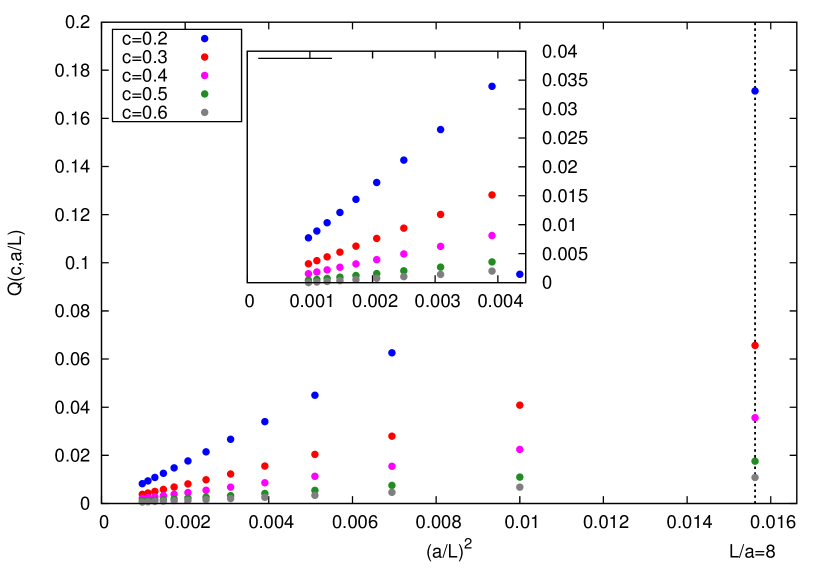
Figure 2: Cutoff effects to leading order of perturbation theory in the twisted gradient flow coupling. As we see, for $c\in[0.3-0.5]$ cutoff effects are below the 7% for an $L/a=8$ lattice.

These figures may lead to the conclusion that a large value of $c$ is optimal. But from the point of view of lattice simulations, it is known Fritzsch:2013je that larger values of $c$ lead to larger statistical errors when computing the coupling via lattice simulations. For the typical lattice sizes ($L/a\sim 10-20$) that one uses in step scaling studies the values $c\in[0.3,0.5]$ seem reasonable.

4.2 Improved coupling definition

If one is computing $t^{2}\langle E(t)\rangle$ non-perturbatively via lattice simulations, and one is using the Wilson action, the Wilson flow and the clover observable for the evaluation of the energy density observable, one can alternatively define the coupling via

$$g_{T}^{2}(L)=\hat{\mathcal{N}}_{T}^{-1}(c,a/L)t^{2}\langle E(t)\rangle\Big{|}_{t=c^{2}L^{2}/8}\,.$$ (72)

This last coupling definition has the same properties, but one expects an improved scaling towards the continuum limit, since the leading order cutoff effects $\propto g_{0}^{2}$ have been removed thanks to the lattice factor $\hat{\mathcal{N}}_{T}(c,a/L)$.

In a similar way, any choice of discretizations that define a coupling can be normalized with a factor computed on the lattice (cf. section 3.2.3), leading to an improved scaling towards the continuum.

5 $SU(2)$ running coupling

In this section we will compute the running coupling in $SU(2)$ pure gauge theory to test if the twisted coupling definition is applicable for step scaling studies.

We will first recall the general strategy, introduced in Luscher:1991wu , of the recursive procedure involved in the computation of the running coupling. The process starts with a non-perturbative coupling definition that depends on no scale other than the linear size of a finite-volume box. Of course in our case this role will be played by the twisted gradient flow coupling $g^{2}_{\rm TGF}(L)$. The step scaling function tells us how much the coupling changes when the renormalization scale is changed by a factor $s$

$$\sigma_{s}(g^{2}(L))=g^{2}(sL)\,.$$ (73)

Therefore it is a discrete version of the $\beta-$function. The value $s=1/2$ is a typical choice, and is the one we will use for now on, although the basic idea is the same for any other value. If one knows how much is the coupling at a renormalization scale that corresponds to a large volume (lets call it $L_{\rm max}$), and one knows the step scaling function, then one can obtain the value of the coupling at scales $L_{\rm max}/2^{k}$ for $k=1,2,\dots$. Eventually, one will reach a very small box size (very large energy scale), where asymptotic freedom guarantees that one can safely make contact with perturbation theory.

To compute the step scaling function numerically one starts by measuring the coupling on some lattice of size $L/a$. The step scaling function is easily obtained by simply measuring the coupling on a lattice half as big ($L/(2a)$) while keeping the rest of the bare parameters constant. The step scaling function computed in this naive way will carry an implicit dependence of the lattice spacing (the cutoff), and therefore defines a lattice step scaling function

$$\Sigma(g^{2}(L),a/L)\,.$$ (74)

In order to obtain the continuum step scaling function $\sigma(g^{2}(L))$, one simulates several pairs of lattices and takes a continuum limit:

$$\sigma(u)=\lim_{a/L\rightarrow 0}\Sigma(u,a/L)\,.$$ (75)

5.1 Numerical computation of the step scaling function and running coupling

5.1.1 Simulation details

We will simulate $SU(2)$ YM theory using the Wilson action

$$S=\frac{\beta}{4}\sum_{\rm p}{\rm Tr}\left\{1-U_{\rm p}\right\}$$ (76)

where the sum runs over all oriented plaquettes. We simulate lattices of size $L/a=20,24,30,36$, and in order to compute the step scaling function also lattices of half this size ($L/a=10,12,15,18$). The range of values of $\beta$ (between 2.75 and 12.0) translate to renormalized couplings $g_{\rm TGF}^{2}(L)$ between 7.5 and 0.6 (for $c=0.3$), enough to cover both the non-perturbative and perturbative regions of the theory. Appendix A collects the values of the $g^{2}_{\rm TGF}(L)$ of our simulations.

We will use a combination of heatbath Creutz:1980zw ; Fabricius:1984wp ; Kennedy:1985nu and overrelaxation Creutz:1987xi as suggested in Wolff:1992nq . In particular we choose to do one heatbath sweep followed by $L/a$ overrelaxation sweeps. Since measuring the coupling (i.e. integrating the flow equations) is numerically more expensive than the Monte Carlo updates, we repeat this process 50 times between measurements.

In total we collect 2048 measurements of the coupling for each lattice size, each value of $\beta$, and several values of $c\in[0.3,0.5]$. These measurements are collected in $N_{r}$ parallel runs (replica) of length $N_{\rm MC}$ each so that $N_{r}\times N_{\rm MC}=2048$. We check that there are no autocorrelation between measurements (i.e. $\tau_{\rm int}=0.5$ within errors), even for our larger lattices and larger values of $c$. We conclude that we can safely consider the measurements independent.

The Wilson flow equations are integrated using the adaptive step size integrator described in appendix D of Fritzsch:2013je . With this scheme we make sure that the integration error in each step is not larger than $10^{-6}$.

5.1.2 Data analysis

For each $L/a$ we have computed the value of the twisted gradient flow coupling at different values of $\beta$ (we call it $g^{2}_{\rm TGF}(\beta;L/a)$). These data are fitted to a Padé-like ansatz

$$g^{2}_{\rm TGF}(\beta;L/a)=\frac{4}{\beta}\quad\frac{\sum_{n=0}^{M-1}a_{n}\beta^{n}+\beta^{M}}{\sum_{n=0}^{M-1}b_{n}\beta^{n}+\beta^{M}}\,.$$ (77)

This fit imposes the one-loop constraint to the data (i.e. $g^{2}_{\rm TGF}(\beta;L/a)\rightarrow 4/\beta$ at large $\beta$), and has a total of $2M$ free fit parameters.

Alternatively, and to estimate the dependence of our results on the choice of functional form used to fit the data, we use a different Padé inspired functional form

$$g^{2}_{\rm TGF}(\beta;L/a)=\frac{4}{\beta}\quad\frac{1}{1+\sum_{n=1}^{M}c_{n}/\beta^{n}}\,,$$ (78)

that also ensures the correct one-loop behavior at large $\beta$.

We obtain good fits ($\chi^{2}/{\rm ndof}\sim 0.6-1.9$) with $M=2$ when using the functional form of Eq. 77 to fit the lattice data (i.e. 4 fitting parameters). When using the functional form of Eq.78 we need $M=4$ to accurately describe the data on the small lattices ($L/a=10,12$) and $M=6$ for the larger ones ($L/a=15,18,20,24,30,36$). It is important to stress that the data are statistically uncorrelated, since they correspond to different simulations.

In the figures 3 we show a couple of these fits. Our worst fit corresponds to the $L/a=24$ lattice and the Pade fit gives a $\chi^{2}/{\rm ndof}=1.69$, while the Taylor fit results in a fit quality of $\chi^{2}/{\rm ndof}=1.9$. We see how in this case the two different functional forms interpolate differently between the data, giving us confidence that if one estimates the error of the interpolation using both functional forms, one will be on the safe side.

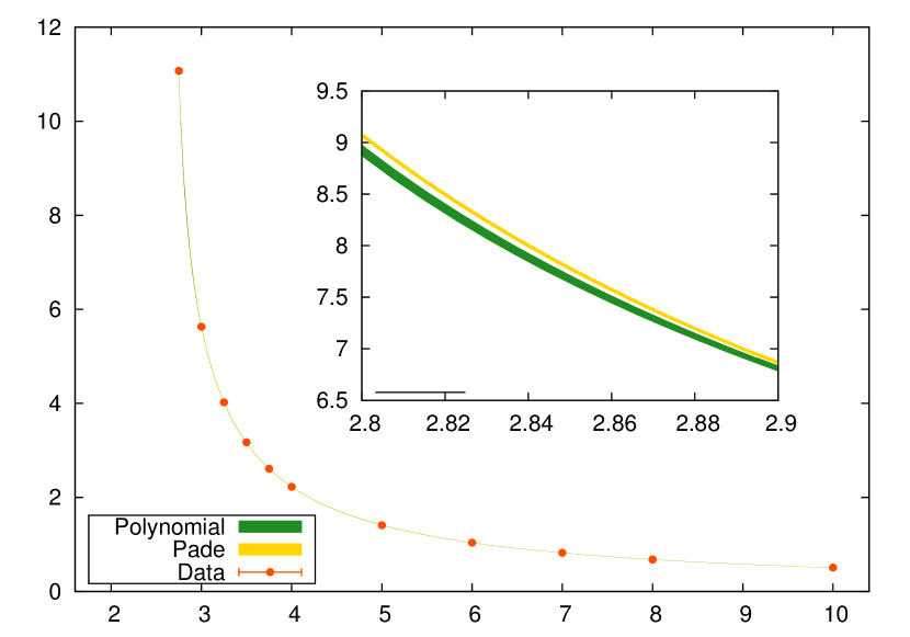
(a)

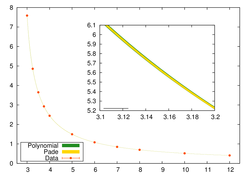
(b)

Figure 3: Some examples of our fits to interpolate the values of the renormalized coupling for different values of $\beta$. (a): Our worst fits corresponds to the $L/a=24$. As we can see there is a difference between the different interpolating functions between the data points. We stress that this systematic effects is taken into account in our analysis by using both functional forms to estimate the error of the interpolations (see the text for more details). (b): Fits to the data of the $L/a=36$ lattice. As we can see, in this case both interpolating functions agree within errors, although the polynomial fits tends to have larger errors.

We use resampling methods to propagate errors by using 4000 bootstrap samples. All fitting parameters derived from our original data are computed for each bootstrap sample. Interpolation points are computed for each bootstrap sample and each functional form. The final error of the interpolated point is computed using both functional forms and all bootstrap samples, and therefore takes into account not only the statistical uncertainty, but also the systematic effect due to the dependence of the interpolating functional form.

5.1.3 Step scaling function

We will first show the continuum extrapolations of the step scaling function $\Sigma(u,a/L)$ at some representative values of $u=7.5,3.75,1.5$. Figure 4 shows that these extrapolations are mild. We have used the value $c=0.3$ that gives a precision in the data for the renormalized coupling between $0.15\%$ and $0.25\%$.

One of the advantages of the use of the twisted boundary conditions is the absence of $\mathcal{O}(a)$ cutoff effects, that are present for example in the Schrödinger functional due to boundary effects. Here the invariance under translations guarantee that the continuum limit can be safely taken by a linear extrapolation in $(a/L)^{2}$.

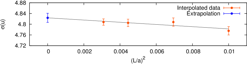
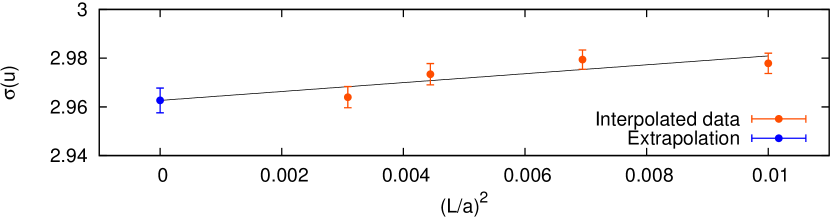
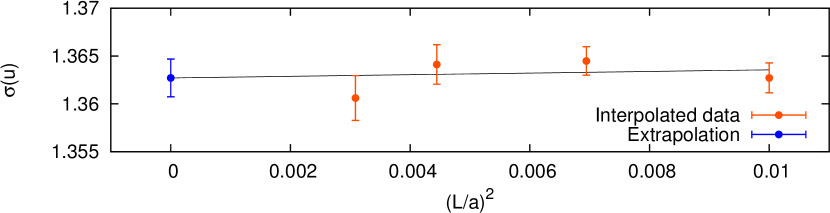
Figure 4: Examples of the continuum extrapolation of the step scaling function. The three figures corresponds (from top to bottom) to the values $u=7.5,3.75,1.5$. We recall that we use a scale factor $s=1/2$, and the scheme is defined by the parameter $c=0.3$.

5.1.4 Running coupling

As a final application, we will compute the running coupling. We will fix the scheme by setting $c=0.3$. We start our recursion in a volume $L_{\rm max}$ defined by the condition

$$g^{2}_{\rm TGF}(L_{\rm max})\Big{|}_{c=0.3}=7.5\,.$$ (79)

The lattice step scaling function and its continuum limit is computed as described in the previous sections. As figure 4 shows, the extrapolations towards the continuum are rather flat. The continuum limit values are used to further compute the values of the step scaling function at larger renormalization scales (smaller volumes), up to $L_{\rm min}=L_{\rm max}/2^{26}$, where $g^{2}_{\rm TGF}(L_{\rm min})|_{c=0.3}=0.5324(84)$.

Since the same functional form (fitting parameters) are used recursively to compute the values of the coupling at different scales, one has to propagate errors taking into account the correlations correctly. This is done in the spirit of the resampling methods in the most naive way: one uses as input for the coupling at a scale $L$ all the bootstrap samples of the coupling from the scale $2L$. We recall here that these bootstrap samples carry the information not only of the statistical uncertainties, but also of the dependence of our results on the functional form chosen to fit the data. Our results have carefully taken into account the two sources of systematic uncertainty: the continuum extrapolation and the choice of fitting function for our lattice data.

Figure 5 shows the running of the coupling from the low energies to the high energies, over a factor $2^{26}$ change in scale, while table 2 contains the numerical values of the coupling at different renormalization scales. The fact that the absolute error in the renormalized coupling tends to be constant a large energies (small volumes), is a consequence of the error propagation, that dominates for large energies the error budget.

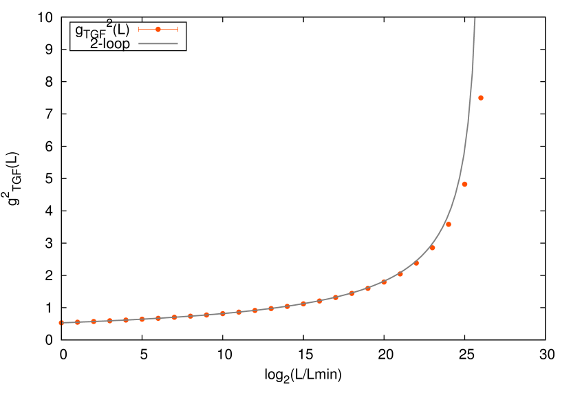
Figure 5: $g^{2}_{\rm TGF}(L)$ as a function of the renormalization scale $\log(L/L_{\rm min})$, and a comparison with the two loop perturbative prediction. Errors are plotted, but compatible with the size of the points.

As a further consistency test, we have repeated the full running of the coupling using as scale factor to define the step scaling function $s=2$ (i.e. we run from high to low energies), obtaining consistent results.

$L=L_{\rm max}/2^{k}$	$k=0$	$k=1$	$k=2$	$k=3$	$k=4$	$k=5$
$g^{2}_{\rm TGF}(L)$	7.5	4.824(17)	3.581(15)	2.858(12)	2.383(10)	2.0464(95)
$L=L_{\rm max}/2^{k}$	$k=6$	$k=7$	$k=8$	$k=9$	$k=10$	$k=11$
$g^{2}_{\rm TGF}(L)$	1.7949(94)	1.5995(94)	1.4432(93)	1.3153(92)	1.2085(90)	1.1181(89)
$L=L_{\rm max}/2^{k}$	$k=12$	$k=13$	$k=14$	$k=15$	$k=16$	$k=17$
$g^{2}_{\rm TGF}(L)$	1.0405(87)	0.9732(86)	0.9143(84)	0.8621(83)	0.8158(83)	0.7742(82)
$L=L_{\rm max}/2^{k}$	$k=18$	$k=19$	$k=20$	$k=21$	$k=22$	$k=23$
$g^{2}_{\rm TGF}(L)$	0.7368(82)	0.7028(82)	0.6720(82)	0.6437(82)	0.6178(82)	0.5939(83)
$L=L_{\rm max}/2^{k}$	$k=24$	$k=25$	$k=26$
$g^{2}_{\rm TGF}(L)$	0.5718(83)	0.5514(84)	0.5324(84)

Table 2: Values of the renormalized twisted gradient flow coupling as a funtion of the renormalization scale $\mu=1/cL$ for $c=0.3$. The final error at large scales (small volumes) is dominated by the error propagation.

The $\Lambda$ parameter can be extracted, in units of $L_{\rm max}$ via

$$\Lambda=\mu(\beta_{0}g^{2}(\mu))^{-\beta_{1}/2\beta_{0}^{2}}e^{-1/2\beta_{0}g^{2}(\mu)}e^{-\int_{0}^{g^{2}(\mu)}\left\{\frac{1}{\beta(x)}+\frac{1}{\beta_{0}x^{3}}-\frac{\beta_{1}}{\beta_{0}^{2}x}\right\}}\,,$$ (80)

using that $\mu=1/cL$. The previous formula is exact, but the last exponential is essentially unknown analytically. Nevertheless if one uses a value of $g^{2}_{\rm TGF}(L)$ where the difference between the two loop and the non-perturbative results are negligible, the effect of the last exponential is also negligible. Of course this is more certain the smaller the coupling, but since the relative error of the coupling grows as the coupling decreases, this would translate in a larger error for the $\Lambda$ parameter. Below we quote a couple of values as example.

$$\Lambda L_{\rm max}=1.509(44)\quad(@g_{TGF}^{2}(L)=1.7949(94))\,,$$

$$\Lambda L_{\rm max}=1.57(13)\quad(@g_{TGF}^{2}(L)=1.0405(87))\,.$$

We want to end this section with a small comment on the use of different values of $c$. The main point has already been raised in Fritzsch:2013je : the larger the value of $c$, the larger the (relative) statistical error of the coupling, but the scaling towards the continuum seems better. This general behavior is consistent with the leading order in perturbation theory as we have seen. We will simply say that the relative error in the raw data increases with $c$, and roughly one can say that for $c=0.4$ the relative error is two times larger than for $c=0.3$, while for $c=0.5$ the error is three times larger. This statement seem to hold true independently of the volume (i.e. of the value of $g^{2}_{\rm TGF}$).

6 Conclusions

In this work we have studied the YM gradient flow for fields obeying twisted boundary conditions on a 4D torus. The energy density of the flow field at positive flow time is used to define a non-perturbative coupling at a scale given by the flow time. Moreover one can make the flow time scale with the finite size of the box. In this way one obtains a coupling that depends only on a scale given by the size of the torus, and the usual techniques of step scaling can be applied.

The perturbative behavior of the energy density of the flow field is computed to leading order both in the lattice and in the continuum. This allows us to estimate the size of cutoff effects of the coupling to leading order in perturbation theory. Results are consistent with other definitions of the running coupling using the gradient flow. Cutoff effects are mild.

In order to state the validity of this coupling definition beyond perturbation theory we have performed a numerical study in pure gauge $SU(2)$. We have computed the running of the coupling from the very perturbative regime $g^{2}\sim 0.5$ to the non perturbative one $g^{2}\sim 7.5$, over a change by a factor $2^{26}$ in scale. We have used lattices of sizes $L/a=10-36$. The statistical precision that one can achieve with this coupling definition is very high: 2048 independent measurements are enough to achieve a sub-percent precision ($0.15-0.25\%$). This precision is roughly independent of the physical volume, the value of the coupling or the lattice size. We have also shown that the continuum extrapolations of the step scaling function are rather flat. Moreover we have shown that this techniques can be used to reliably extract the $\Lambda$ parameter.

The same coupling definition can be used if fermions are coupled to the gauge field. But the consistency of the twisted boundary conditions imposes a constraint on the number of fermions in the fundamental representation that we can use. In particular, what arguably is the most interesting application of these techiniques, namely the coupling constant of QCD (gauge group $SU(3)$ with $N_{f}=4$ fermions in the fundamental representation) can not be attacked with this method. Nevertheless there are many applications of this work. On one hand $N_{f}=3$ flavour of quarks in the fundamental representation is already interesting for the strong interations. But it is probably in the context of conformal theories and physics beyond the standard model, with models like $SU(3)$ with $N_{f}=12$ fermions in the fundamental representation, or with adjoint fermions, where the nice properties of this coupling definition (automatic $\mathcal{O}(a)$ improvement, analyticity and high statistical precision) can have a higher impact. In particular the setup with twisted boundary conditions have already been used for step scaling studies in the TPL scheme Lin:2012iw ; Itou:2012qn . In this particular case the use of the gradient flow observable will lead to more precise results, as we have already seen in some preliminary results in the last lattice conference linconf . One can also consider the application of the same ideas to other choices of twisted boundary conditions. This is specially interesting in the context of reduced models, as we have also seen recently liamconf .

Appendix A Raw values of $g_{TGF}^{2}$

All the values quoted in this appendix are computed using Eq. 72. Simulations are performed as described in section 5.

$\beta$	10	12	15	18	$L/a$
12.0	$0.39194(60)$	$0.39465(61)$	$0.39813(62)$	$0.39974(59)$
10.0	$0.48769(76)$	$0.49211(74)$	$0.49688(76)$	$0.49945(76)$
8.0	$0.6455(10)$	$0.6517(10)$	$0.6605(10)$	$0.6693(10)$
7.0	$0.7701(12)$	$0.7824(12)$	$0.7945(13)$	$0.8055(13)$
6.0	$0.9574(15)$	$0.9738(16)$	$0.9934(16)$	$1.0087(16)$
5.0	$1.2644(20)$	$1.2933(22)$	$1.3269(22)$	$1.3573(22)$
4.0	$1.8747(31)$	$1.9390(33)$	$2.0194(36)$	$2.0883(36)$
3.75	$2.1336(38)$	$2.2138(39)$	$2.3259(41)$	$2.4263(43)$
3.5	$2.4910(44)$	$2.5971(47)$	$2.7584(52)$	$2.8999(53)$
3.25	$2.9803(55)$	$3.1476(59)$	$3.4002(66)$	$3.6192(70)$
3.0	$3.7453(73)$	$4.0287(79)$	$4.4214(87)$	$4.8287(99)$
2.75	$5.119(11)$	$5.684(13)$	$6.622(16)$	$7.745(21)$

$\beta$	20	24	30	36	$L/a$
12.0	$0.40162(60)$	$-$	$0.40772(61)$	$0.41078(63)$
10.0	$0.50340(76)$	$0.50786(77)$	$0.51280(82)$	$0.51809(85)$
8.0	$0.6741(11)$	$0.6794(11)$	$0.6900(11)$	$0.6987(11)$
7.0	$0.8125(13)$	$0.8240(13)$	$0.8369(13)$	$0.8497(13)$
6.0	$1.0222(17)$	$1.0379(17)$	$1.0609(17)$	$1.0819(18)$
5.0	$1.3767(23)$	$1.4091(23)$	$1.4562(25)$	$1.4968(25)$
4.0	$2.1439(39)$	$2.2260(41)$	$2.3453(42)$	$2.4465(43)$
3.75	$2.5047(47)$	$2.6107(48)$	$2.7636(52)$	$2.9277(54)$
3.5	$3.0037(57)$	$3.1720(60)$	$3.4170(66)$	$3.6494(70)$
3.25	$3.7581(75)$	$4.0224(75)$	$4.4397(86)$	$4.8568(98)$
3.0	$5.088(11)$	$5.630(12)$	$6.573(16)$	$7.587(20)$
2.75	$8.699(25)$	$11.072(34)$	$15.817(44)$	$-$

Table 3: Raw values of $g^{2}_{\rm TGF}(\beta;L/a)$.

References

- (1) D. J. Gross and F. Wilczek, Ultraviolet behavior of non-abelian gauge theories, Phys. Rev. Lett. 30 (Jun, 1973) 1343–1346.
- (2) H. D. Politzer, Reliable perturbative results for strong interactions?, Phys. Rev. Lett. 30 (Jun, 1973) 1346–1349.
- (3) M. Lüscher, P. Weisz, and U. Wolff, A Numerical method to compute the running coupling in asymptotically free theories, Nucl.Phys. B359 (1991) 221–243.
- (4) M. Lüscher, R. Narayanan, P. Weisz, and U. Wolff, The Schrödinger Functional: a renormalizable probe for non-abelian gauge theories, Nucl.Phys. B384 (1992) 168–228, [hep-lat/9207009].
- (5) G. de Divitiis, R. Frezzotti, M. Guagnelli, and R. Petronzio, Non-perturbative determination of the running coupling constant in quenched SU(2), Nucl.Phys. B433 (1995) 390–402, [hep-lat/9407028].
- (6) M. Luscher, R. Sommer, U. Wolff, and P. Weisz, Computation of the running coupling in the SU(2) Yang-Mills theory, Nucl.Phys. B389 (1993) 247–264, [hep-lat/9207010].
- (7) M. Lüscher, R. Sommer, P. Weisz, and U. Wolff, A precise determination of the running coupling in the SU(3) Yang-Mills theory, Nucl.Phys. B413 (1994) 481–502, [hep-lat/9309005].
- (8) ALPHA Collaboration, M. Della Morte et al., Computation of the strong coupling in QCD with two dynamical flavors, Nucl.Phys. B713 (2005) 378–406, [hep-lat/0411025].
- (9) ALPHA Collaboration, F. Tekin, R. Sommer, and U. Wolff, The running coupling of QCD with four flavors, Nucl.Phys. B840 (2010) 114–128, [arXiv:1006.0672].
- (10) S. Sint, On the Schrödinger functional in QCD, Nucl.Phys. B421 (1994) 135–158, [hep-lat/9312079].
- (11) S. Sint, One loop renormalization of the QCD Schrödinger functional, Nucl.Phys. B451 (1995) 416–444, [hep-lat/9504005].
- (12) S. Sint, The Chirally rotated Schrödinger functional with Wilson fermions and automatic O(a) improvement, Nucl.Phys. B847 (2011) 491–531, [arXiv:1008.4857].
- (13) R. Frezzotti and G. Rossi, Chirally improving Wilson fermions. 1. O(a) improvement, JHEP 0408 (2004) 007, [hep-lat/0306014].
- (14) M. Lüscher, Properties and uses of the Wilson flow in lattice QCD, JHEP 1008 (2010) 071, [arXiv:1006.4518].
- (15) M. Lüscher and P. Weisz, Perturbative analysis of the gradient flow in non-abelian gauge theories, JHEP 1102 (2011) 051, [arXiv:1101.0963].
- (16) Z. Fodor, K. Holland, J. Kuti, D. Nogradi, and C. H. Wong, The Yang-Mills gradient flow in finite volume, JHEP 1211 (2012) 007, [arXiv:1208.1051].
- (17) A. Gonzalez-Arroyo, J. Jurkiewicz, and C. Korthals-Altes, Ground state metamorphosis for Yang-Mills fields on a finite periodic lattice, .
- (18) P. van Baal, Gauge theory in a finite volume, Acta Phys.Polon. B20 (1989) 295–312.
- (19) P. Fritzsch and A. Ramos, The gradient flow coupling in the Schr dinger Functional, JHEP 1310 (2013) 008, [arXiv:1301.4388].
- (20) ALPHA Collaboration, S. Schaefer, R. Sommer, and F. Virotta, Critical slowing down and error analysis in lattice QCD simulations, Nucl. Phys. B845 (2011) 93–119, [arXiv:1009.5228].
- (21) M. Lüscher and S. Schaefer, Lattice QCD without topology barriers, JHEP 1107 (2011) 036, [arXiv:1105.4749].
- (22) P. Fritzsch, A. Ramos, and F. Stollenwerk, Critical slowing down and the gradient flow coupling in the Schrödinger functional, PoS Lattice2013 (2013) 461, [arXiv:1311.7304].
- (23) M. L scher, Step scaling and the Yang-Mills gradient flow, JHEP 1406 (2014) 105, [arXiv:1404.5930].
- (24) M. Lüscher and S. Schaefer, Lattice QCD with open boundary conditions and twisted-mass reweighting, Comput.Phys.Commun. 184 (2013) 519–528, [arXiv:1206.2809].
- (25) A. González-Arroyo, Yang-Mills fields on the 4-dimensional Torus. Part I: Classical Theory, World Scientific. Proceedings of the Peñiscola 1997 advanced school on non-perturbative quantum field physics (1998) Singapore, [hep-th/9807108].
- (26) M. García Pérez, A. González-Arroyo, and M. Okawa, Spatial volume dependence for 2+1 dimensional SU(N) Yang-Mills theory, JHEP 1309 (2013) 003, [arXiv:1307.5254].
- (27) G. ’t Hooft, A property of electric and magnetic flux in nonabelian gauge theories, Nucl. Phys. B153 (1979) 141.
- (28) M. Luscher and P. Weisz, Efficient Numerical Techniques for Perturbative Lattice Gauge Theory Computations, Nucl.Phys. B266 (1986) 309.
- (29) G. Parisi, Prolegomena to any future computer evaluation of the QCD mass spectrum, Cargese Summer Inst. 1983:0531 (1984).
- (30) R. Narayanan and H. Neuberger, Infinite N phase transitions in continuum Wilson loop operators, JHEP 0603 (2006) 064, [hep-th/0601210].
- (31) M. Lüscher, Trivializing maps, the Wilson flow and the HMC algorithm, Commun.Math.Phys. 293 (2010) 899–919, [arXiv:0907.5491].
- (32) M. Luscher, Chiral symmetry and the Yang–Mills gradient flow, JHEP 1304 (2013) 123, [arXiv:1302.5246].
- (33) M. Creutz, Monte Carlo Study of Quantized SU(2) Gauge Theory, Phys.Rev. D21 (1980) 2308–2315.
- (34) K. Fabricius and O. Haan, Heat Bath Method for the Twisted Eguchi-Kawai Model, Phys.Lett. B143 (1984) 459.
- (35) A. Kennedy and B. Pendleton, Improved Heat Bath Method for Monte Carlo Calculations in Lattice Gauge Theories, Phys.Lett. B156 (1985) 393–399.
- (36) M. Creutz, Overrelaxation and Monte Carlo Simulation, Phys.Rev. D36 (1987) 515.
- (37) U. Wolff, Dynamics of hybrid overrelaxation in the Gaussian model, Phys.Lett. B288 (1992) 166–170.
- (38) C.-J. D. Lin, K. Ogawa, H. Ohki, and E. Shintani, Lattice study of infrared behaviour in SU(3) gauge theory with twelve massless flavours, JHEP 1208 (2012) 096, [arXiv:1205.6076].
- (39) E. Itou, Properties of the twisted Polyakov loop coupling and the infrared fixed point in the SU(3) gauge theories, PTEP 2013 (2013), no. 8 083B01, [arXiv:1212.1353].
- (40) D. Lin, SU(3) gauge theory with 12 flavours in a twisted box., Talk at The 32nd International Symposium on Lattice Field Theory (2014).
- (41) L. Keegan, TEK twisted gradient flow running coupling., Talk at The 32nd International Symposium on Lattice Field Theory (2014).