Local and nonlocal dynamics in superfluid turbulence

Abstract

In turbulent superfluid He II, the quantized vortex lines interact via the classical Biot–Savart law to form a complicated vortex tangle. We show that vortex tangles with the same vortex line density will have different energy spectra, depending on the normal fluid which feeds energy into the superfluid component, and identify the spectral signature of two forms of superfluid turbulence: Kolmogorov tangles and Vinen tangles. By decomposing the superfluid velocity field into local and nonlocal contributions, we find that in Vinen tangles the motion of vortex lines depends mainly on the local curvature, whereas in Kolmogorov tangles the long-range vortex interaction is dominant and leads to the formation of clustering of lines, in analogy to the ’worms‘ of ordinary turbulence.

I Introduction

The hydrodynamics of helium II is noteworthy for two reasons: its two-fluid nature (an inviscid superfluid and a viscous normal fluid), and the fact that superfluid vorticity is constrained to thin, discrete vortex lines of fixed (quantized) circulation Donnelly ; in ordinary (classical) fluids, by contrast, the vorticity is a continuous field. Turbulence in helium II (called superfluid turbulence, or quantum turbulence) consists of a three-dimensional tangle of interacting vortex lines. The properties of this new form of turbulence and current thinking (in terms of theory and experiments) have been recently reviewed Barenghi-Skrbek-Sreeni ; Nemirovskii .

Under certain conditions, it has been argued Vinen-Niemela ; Skrbek-Sreeni that the turbulent tangle is characterized by a single length scale, the average distance $\ell$ between the vortex lines, which is inferred from the experimentally observed vortex line density $L$ (length of vortex line per unit volume) as $\ell\approx L^{-1/2}$. Models based on this property describe fairly well the pioneering experiments of Vinen Vinen , in which an applied heat flux drives the superfluid and the normal fluid in opposite directions (thermal counterflow). More recently, such ‘Vinen’ tangles were created at very low temperatures by short injections of ions Walmsley-Golov , exhibiting the characteristic decay $L\sim t^{-1/2}$ predicted by Vinen Baggaley-ultraquantum .

Under different conditions, however, the experimental evidence is consistent with a more structured vortex tangle Vinen-Niemela ; Volovik , where the kinetic energy is distributed over a range of length scales according to the same Kolmogorov law which governs ordinary turbulence. ‘Kolmogorov’ tangles have been generated at high temperatures by stirring liquid helium with grids Donnelly-grid or propellers Tabeling ; Salort , and at very low temperatures by an intense injection of ions Walmsley-Golov , exhibiting the decay $L\sim t^{-3/2}$ expected from the energy spectrum Donnelly-grid ; Baggaley-ultraquantum .

The experimental evidence for these two forms of superfluid turbulence is only indirect and arises from macroscopic observables averaged over the experimental cell, such as pressure Tabeling ; Salort and vortex line density Donnelly-grid , not from direct visualization of vortex lines. In a recent paper Sherwin we have characterized the energy spectrum of the two forms of turbulence, and showed that ’Kolmogorov’ turbulence contains metastable, coherent vortex structures Baggaley-structures ; Baggaley-Laurie , similar perhaps to the ‘worms’ which are observed in ordinary turbulence Frisch . The aim of this work is to go a step further, and look for the dynamical origin of the reported spectral difference and coherent structures.

It is well known Saffman that in an incompressible fluid the velocity field ${\bf{v}}$ is determined by the instantaneous distribution of vorticity $\omega$ via the Biot-Savart law:

$${\bf{v}}({\bf{x}})=\frac{1}{4\pi}\int\frac{{\mbox{\boldmath$\omega$}}({\bf{x}}^{\prime})\times({\bf{x}}-{\bf{x}}^{\prime})}{|{\bf{x}}-{\bf{x}}^{\prime}|^{3}}d^{3}{\bf{x}}^{\prime}$$ (1)

where the integral extends over the entire flow. The question which we address is whether the velocity at the point ${\bf{x}}$ is mainly determined by the (local) vorticity near ${\bf{x}}$ or by (nonlocal) contributions from further away. Since the quantization of the circulation implies that the velocity field around a vortex line is strictly $1/r$ (where $r$ is the radial distance from the line), from the predominance of local effects we would infer that the vorticity is randomly distributed and nonlocal effects cancel each other out; conversely, the predominance of nonlocal effects would suggest the existence of coherence structures.

If the vorticity were a continuous field, the distinction between local and nonlocal would involve an arbitrary distance, however in our problem the concentrated nature of vorticity introduces a natural distinction between local and nonlocal contributions, as we shall see.

II Method

The two most popular models Barenghi-Skrbek-Sreeni for studying superfluid turbulence are the Gross-Pitaevskii equation (GPE) and the Vortex Filament Model (VFM). Each has advantages and disadvantages. The main advantage of the GPE over the VFM is that vortex reconnections are solutions of the equation of motion and do not require an ad–hoc algorithmic procedure. On the other hand, the experimental context of our interest is liquid helium at intermediate temperatures where the effects of the friction are important (at the chosen value $T=1.9~{}K$, typical of experiments, the normal fluid fraction is 42 percent). We must keep in mind that, although the GPE is a good quantitative model of weakly interacting atomic gases, it is only an idealized model of liquid helium; moreover, the GPE applies only at very low temperatures, and there is not yet a consensusProukakis2008 on its finite-temperature generalizations. This is why, following the approach of SchwarzSchwarz , we choose to use the VFM and model superfluid vortex lines as space curves ${\bf{s}}(\xi,t)$ (where $t$ is time and $\xi$ is arc length) of infinitesimal thickness and circulation $\kappa=9.97\times 10^{-4}~{}\rm cm^{2}/s$ which move according to

$$\frac{ds}{dt}={\bf{v}}_{s}+\alpha{\bf{s}}^{\prime}\times({\bf{v}}_{n}^{ext}-{\bf{v}}_{s})-\alpha^{\prime}{\bf{s}}^{\prime}\times[{\bf{s}}^{\prime}\times({\bf{v}}_{n}^{ext}-{\bf{v}}_{s})].$$ (2)

Here $\alpha$ and $\alpha^{\prime}$ are temperature-dependent friction coefficients BDV ; DB , ${\bf{v}}_{n}$ is the normal fluid velocity, and a prime denotes derivative with respect to arc length (hence ${\bf{s}}^{\prime}=d{\bf{s}}/d\xi$ is the local unit tangent vector, and $C=|{\bf{s}}^{\prime\prime}|$ is the local curvature; the radius of curvature, $R=1/C$, is the radius of the osculating circle at the point ${\bf{s}}$). The superfluid velocity consists of two parts: ${\bf{v}}_{s}={\bf{v}}_{s}^{ext}+{\bf{v}}_{s}^{self}$. The former ${\bf{v}}_{s}^{ext}$ represents any externally applied superflow; the latter ${\bf{v}}_{s}^{self}$ the self-induced velocity at the point ${\bf{s}}$, results from Equation 1 in the limit of concentrated vorticity:

$${\bf{v}}_{s}^{self}({\bf{s}})=-\frac{\kappa}{4\pi}\oint_{\mathcal{L}}\frac{({\bf{s}}-{\bf{r}})}{|{\bf{s}}-{\bf{r}}|^{3}}\times{\bf{dr}},$$ (3)

where the line integral extends over the entire vortex configuration $\mathcal{L}$.

We discretised the vortex lines into a large number of points ${\bf{s}}_{j}$ ($j=1,\cdots N$). The minimal separation $\delta$ between the points is such that the vortex curves are sufficiently smooth (at the temperatures of interest here, the friction, controlled by the parameters $\alpha$ and $\alpha^{\prime}$, damps out high frequency perturbations called Kelvin waves). The VFM assumes that vortex lines are infinitely thin, thus Eq. (3) is valid only if $|{\bf{s}}-{\bf{r}}|>>a_{0}$ where $a_{0}$ is the vortex core (the region around the vortex axis where the superfluid density drops from its bulk value to zero). Thus the integral diverges if one attempts to find the velocity at ${\bf{r}}={\bf{s}}$. As remarked by Schwarz, the occurrence of a similar problem in classical hydrodynamics is not helpful, since the physics of the vortex core is different. The solution to the problem which was proposed by Schwarz Schwarz1985 and thereafter adopted in the helium literature is based on Taylor expanding the integrand around the singularity and comparing against the well-know expression for the self-induced velocity of a circular ring. In this way he obtained a decomposition of the self-induced velocity at the point ${\bf{s}}_{j}$ (Eq. 3) into the following local and nonlocal contributions:

$${\bf{v}}_{s}^{self}({\bf{s}}_{j})={\bf{v}}_{s}^{loc}({\bf{s}}_{j})+{\bf{v}}_{s}^{non}({\bf{s}}_{j})=\frac{\kappa}{4\pi}\ln\left(\frac{\sqrt{\Delta\xi_{+}\Delta\xi_{-}}}{a_{0}}\right){\bf{s}}^{\prime}_{j}\times{\bf{s}}^{\prime\prime}_{j}+\frac{\kappa}{4\pi}\oint_{\mathcal{L}^{\prime}}\frac{({\bf{s}}_{j}-{\bf{r}})}{|{\bf{s}}_{j}-{\bf{r}}|^{3}}\times{\bf{dr}}$$ (4)

where $\Delta\xi_{+}$ and $\Delta\xi_{-}$ are the arc lengths of the curves between the point ${\bf{s}}_{j}$ and the adjacent points ${\bf{s}}_{j-1}$ and ${\bf{s}}_{j+1}$ along the vortex line. $\mathcal{L}^{\prime}$ is the original vortex configuration $\mathcal{L}$ but now without the section between ${\bf{s}}_{j-1}$ and ${\bf{s}}_{j+1}$. The superfluid vortex core radius $a_{0}\approx 10^{-8}~{}\rm cm$ acts as cutoff parameter. Details and tests of the numerical techniques against the experimental and the numerical literature are published elsewhere Baggaley-reconnections ; Baggaley-stats ; Baggaley-PNAS ; Adachi . Note that the local contribution is proportional to ${\bf{s}}^{\prime}\times{\bf{s}}^{\prime\prime}$, in the binormal direction.

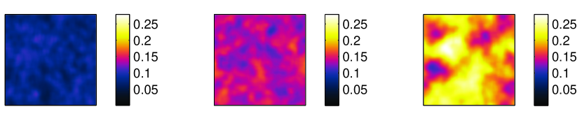
Figure 8: Superfluid energy density $\epsilon_{s}=|{\bf{v}}_{s}|^{2}/2$ smoothed over the average inter-vorex spacing $\ell$, plotted on the $xy$ plane and averaged over $z$. Left: model 1 (uniform normal fluid); middle: model 2 (synthetic turbulence); right: model 3 (frozen Navier-Stokes turbulence). Parameters as in Fig. (2).

All calculations are performed in a cubic periodic domain of size $D=0.1$ using an Adams-Bashforth time-stepping method (with typical time step $\Delta t=5\times 10^{-5}~{}\rm s$), a tree-method Baggaley-tree with opening angle $\theta=0.4$, and typical minimal resolution $\delta=1.6\times 10^{-3}~{}\rm cm$. For example, an increase in the numerical resolution from $\delta=0.0016$ to $\delta=0.0008$ produces a small increase of 2.5% in the importance of the nonlocal contribution in Fig. (8). Moreover, the tests against experiments mentioned above Baggaley-stats ; Baggaley-PNAS ; Adachi , guarantee that the numerical resolution is sufficient, and put the distinction between ${\bf{v}}_{s}^{loc}$ and ${\bf{v}}_{s}^{non}$ on solid ground.

It is known from experiments Bewley2008 and from more microscopic models Koplik ; Zuccher ; Allen2014 that colliding vortex lines reconnect with each other. An algorithmic procedure is introduced to reconnect two vortex lines if they become sufficiently close to each other. This procedure (although arbitrary, unlike the GPE as mentioned before) has been extensively tested Baggaley-reconnections ; various slightly different reconnection algorithms have been proposed and have never been found in disagreement with experimental observations.

We choose a temperature typical of experiments, $T=1.9~{}\rm K$ (corresponding to $\alpha=0.206$ and $\alpha^{\prime}=0.00834$). In all three cases, the initial condition consists of a few seeding vortex loops, which interact and reconnect, quickly generating a turbulent vortex tangle which appears independent of the initial condition.

We study the following three different regimes of superfluid turbulence, characterized by the following forms of the normal fluid’s velocity field ${\bf{v}}_{n}^{ext}$:

1. Uniform normal flow. Firstly, to model turbulence generated by a small heat flux at the blocked end of a channel (thermal counterflow), we impose a uniform normal fluid velocity ${\bf{v}}_{n}^{ext}=V_{n}\hat{\bf x}$ in the x-direction (which we interpret as the direction of the channel) which is proportional to the applied heat flux; to conserve mass, we add a uniform superflow ${\bf{v}}_{s}^{ext}=-(\rho_{n}/\rho_{s})V_{n}\hat{\bf x}$ in the opposite direction, where $\rho_{n}$ and $\rho_{s}$ are respectively the normal fluid and superfluid densities. Eqs. (2) and (4) are solved in the imposed superflow’s reference frame. This model is the most used in the literature, from the pioneering work of Schwarz Schwarz to the recent calculations of Tsubota and collaborators Adachi .

2. Synthetic turbulence. To model turbulence generated by pushing helium through pipes or channels Salort using plungers or bellows or by stirring it with grids Donnelly-grid or propellers Tabeling , we start from the observation that, due to liquid helium’s small viscosity $\mu$, the normal fluid’s Reynolds number ${\rm Re}=VD/\nu_{n}$ is usually large (where $V$ is the rms velocity and $\nu_{n}=\mu/\rho_{n}$ the kinematic viscosity), hence we expect the normal fluid to be turbulent. We assume ${\bf{v}}_{s}^{ext}={\bf 0}$ and Osborne-2006

   $${\bf{v}}_{n}^{ext}({\bf{s}},t)=\sum_{m=1}^{M}({\bf A}_{m}\times{\bf k}_{m}\cos{\phi_{m}}+{\bf B}_{m}\times{\bf k}_{m}\sin{\phi_{m}}),$$ (5)

   where $\phi_{m}={\bf{k}}_{m}\cdot{\bf{s}}+f_{m}t$, ${\bf{k}}_{m}$ are wavevectors and $f_{m}=\sqrt{k^{3}_{m}E(k_{m})}$ are angular frequencies. The random parameters ${\bf A}_{m}$, ${\bf B}_{m}$ and ${\bf k}_{m}$ are chosen so that the normal fluid’s energy spectrum obeys Kolmogorov’s scaling $E(k_{m})\propto k_{m}^{-5/3}$ in the inertial range $k_{1}<k<k_{M}$, where $k_{1}\approx 2\pi/D$ and $k_{M}$ correspond to the outer scale of the turbulence and the dissipation length scale respectively. Then we define the Reynolds number via ${\rm Re}=(k_{M}/k_{1})^{4/3}$. The synthetic turbulent flow defined by Eq. (5) is solenoidal, time-dependent, and compares well with Lagrangian statistics obtained in experiments and direct numerical simulations of the Navier-Stokes equation. It is therefore physically realistic and numerically convenient to model current experiments on grid or propeller generated superfluid turbulence.

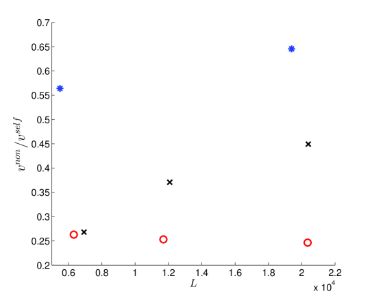
Figure 11: (color online). Ratio $v^{non}/v^{self}$ as a function of vortex line density $L$ $(\rm cm^{-2})$ corresponding to model 1 (uniform normal flow, red circles), model 2 (synthetic normal flow turbulence, black crosses) and model 3 (frozen Navier-Stokes equation, blue stars).

3. Frozen Navier-Stokes turbulence. Synthetic turbulence, being essentially the superposition of random waves, lacks the intense regions of concentrated vorticity which are typical of classical turbulence Frisch . For this reason we consider a third model: a turbulent flow ${\bf{v}}_{n}^{ext}$ obtained by direct numerical simulation (DNS) of the classical Navier-Stokes equation in a periodic box with no mean flow. Since the simultaneous calculation of superfluid vortices and turbulent normal fluid would be prohibitively expensive, we limit ourselves to a time snapshot of ${\bf{v}}_{n}^{ext}$. In other words, we determine the vortex lines under a ’frozen‘ turbulent normal fluid. Our source for the DNS data is the John Hopkins Turbulence Database JHTDB1 ; JHTDB2 , which consists of a velocity field on a $1024^{3}$ spatial mesh. The estimated Reynolds number is ${\rm Re}\approx(L_{0}/\eta_{0})^{4/3}=3205$ where $L_{0}$ is the integral scale and $\eta_{0}$ the Kolmogorov scale. Although ${\rm Re}=3205$ is not a very large Reynolds number, at $T=1.9~{}K$ helium’s viscosity is $\mu=1.347\times 10^{-5}~{}\rm g/(cm~{}s)$, the normal fluid density is $\rho_{n}=0.0611~{}\rm g/cm^{3}$, the kinematic viscosity is $\nu_{n}=\mu/\rho_{n}=0.22\times 10^{-3}~{}\rm cm/s$ DB , and therefore ${\rm Re}=UD/\nu_{n}=3205$ corresponds to the reasonable speed $U=0.7~{}\rm cm/s$ in a typical $D=1~{}\rm cm$ channel. To keep the resulting vortex line density of this model to a computationally practical value, we rescale the velocity components such that they are 60 percent of their original values, thus obtaining the vortex line density $L\approx 20,0000~{}\rm cm^{-2}$. To obtain Fig. 11 the scaling factor is only 45 percent, yielding $L\approx 6,000~{}\rm cm^{-2}$; because of the nonlinearity of the Navier-Stokes equation, this procedure is clearly an approximation but is sufficient for our aim of driving a less intense of more intense vortex tangle.

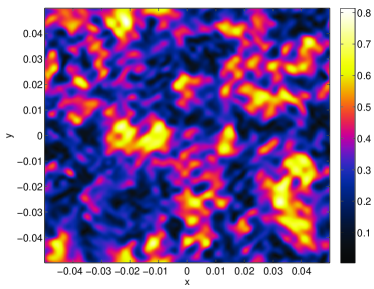
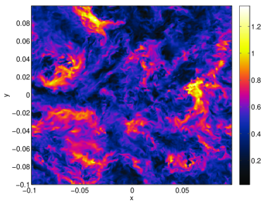
Figure 1: (color online). Magnitude of the driving normal fluid velocity field, $|{\bf{v}}_{n}^{ext}|$, plotted on the $xy$-plane at $z=0$ corresponding to model 2 (synthetic normal flow turbulence, left) and model 3 (frozen Navier-Stokes turbulence, right). The velocity scales (cm/s) are shown at right of each panel. Note the more localized, more intense regions of velocity which are present in model 3.

Fig. 1 shows the magnitude of the normal velocity field plotted (at a fixed time $t$) on the $xy$ plane at $z=0$, corresponding to models 2 and 3 (we do not plot the normal fluid velocity for model 1 because it is uniform). It is apparent that models 1, 2 and 3 represent a progression of increasing complexity of the driving normal flow. In Fig. 1, note in particular the localized regions of strong velocity which appear in model 3.

III Results

The intensity of the turbulence is measured by the vortex line density $L=\Lambda/V$ (where $\Lambda$ is the superfluid vortex length in the volume $V=D^{3}$), which we monitor for a sufficiently long time, such that the properties which we report, refer to a statistically steady state of turbulence fluctuating about a certain average $L$ (we choose parameters so that $L$ is typical of experiments).

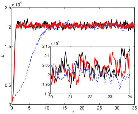
Figure 2: (color online). Evolution of the vortex line density $L$ (cm^-2) vs time $t$ (s) for model 1 (red line, uniform normal flow), model 2 (black line, synthetic normal fluid turbulence) and model 3 (dashed blue line, frozen Navier-Stokes turbulence). The inset displays the oscillations of $L$ vs $t$ in more detail. Parameters: temperature $T=1.9~{}\rm K$, $V_{n}=1~{}\rm cm/s$ (for model 1), ${\rm Re}=79.44$ (for model 2), and ${\rm Re}=3025$ (for model 3).

Fig. 2 shows the initial transient of the vortex line density followed by the saturation to statistically steady-states of turbulence corresponding to model 1 (uniform normal flow), model 2 (synthetic normal flow turbulence) and model 3 (frozen Navier-Stokes turbulence). In all cases, the intensity of the drive is chosen to generate approximately the same vortex line density, $L\approx 20,000~{}\rm cm^{-2}$.

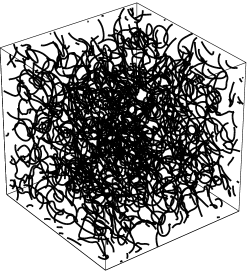
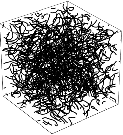
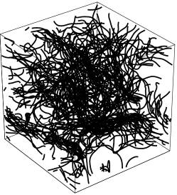
Figure 3: Snapshot of the vortex tangle for model 1 (uniform normal fluid, left), model 2 (synthetic turbulence, middle) and model 3 (frozen Navier-Stokes turbulence, right) at time $t=20~{}\rm s$ (parameters as in Fig. (2).

Snapshots of the vortex tangles are shown in Fig. 3. The vortex tangle driven by the uniform normal fluid (model 1, left) appears visually as the most homogeneous; the vortex tangle driven by the frozen Navier-Stokes turbulence (model 3, right) appears as the least homogeneous. What is not apparent in the figure is the mild anisotropy of the tangle driven by the uniform normal fluid. To quantify this anisotropy, we calculate the projected vortex lengths in the three Cartesian directions ($\Lambda_{x}$, $\Lambda_{y}$, $\Lambda_{z}$) and find $\Lambda_{x}/\Lambda=0.34<\Lambda_{y}/\Lambda=\Lambda_{z}/\Lambda=0.54$ for model 1, confirming a small flattening of the vortices in the yz plane (this effect was discovered by the early investigations of Schwarz Schwarz ). In comparison, models 2 and 3 are more isotropic: for model 2 (tangle driven by synthetic turbulence) we find $\Lambda_{x}/\Lambda=0.50$, $\Lambda_{y}/\Lambda=0.47$ and $\Lambda_{z}/\Lambda=0.49$), and for model 3 (tangle driven by frozen Navier-Stokes turbulence) we obtain $\Lambda_{x}/\Lambda=0.48$, $\Lambda_{y}/\Lambda=0.50$, $\Lambda_{z}/\Lambda=0.49$.

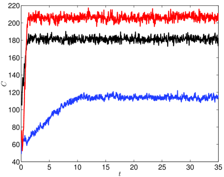
Figure 4: (color online). Average curvature $C$ ($\rm cm^{-1}$) vs time $t$ ($\rm s$) for model 1 (uniform normal flow, red line), model 2 (synthetic turbulence, black line) and model 3 (frozen Navier-Stokes turbulence, dashed blue line). Parameters as in Fig. (2).

Fig. 4 and 5 shows the average curvature $C=<C_{j}>$ (sampled over the discretization points $j=1,\cdots N$) and the distributions of local curvatures $C_{j}=|{\bf{s}}_{j}^{\prime\prime}|$. The tangle generated by model 3 (frozen Navier-Stokes turbulence) has the smallest average curvature: the presence of long lines (large radius of curvature $R=1/|{\bf{s}}^{\prime\prime}|$) is indeed visible in Fig. 2. In terms of curvature, the tangles generated by models 1 and 2 are more similar to each other - the average curvature is almost twice as large as for model 3, indicating that the vortex lines are more in the form of small loops.

However, vortex line density (Fig. 2), visual inspection (Fig. 3) and curvature (Fig. 4 and 5) do not carry information about the orientation of the vortex lines, a crucial ingredient of the dynamics. Fig. 6 shows the energy spectrum $E_{s}(k)$, defined by

$$\frac{1}{V}\int_{V}\frac{1}{2}{\bf v}_{s}^{2}dV=\int_{0}^{\infty}E_{s}(k)dk$$ (6)

where $k$ is the magnitude of the three-dimensional wavevector. The energy spectrum describes the distribution of kinetic energy over the length scales. The spectra of the tangles generated by synthetic normal flow turbulence (model 2) and by the frozen Navier-Stokes turbulence (model 3) are consistent with the classical Kolmogorov scaling $E_{s}(k)\sim k^{-5/3}$ for $k<k_{\ell}=2\pi/\ell$; the kinetic energy is clearly concentrated at the largest length scales (small $k$). In contrast, the spectrum of the tangle generated by the uniform normal fluid (model 1) peaks at the intermediate length scales, and at large wavenumbers is consistent with the shallower $k^{-1}$ dependence of individual vortex lines.

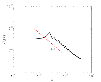
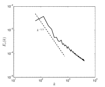
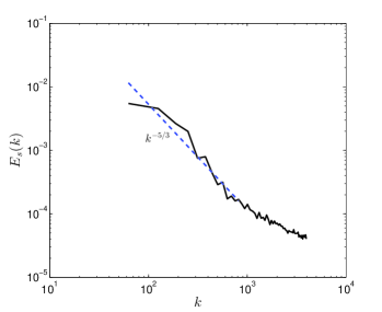
Figure 7: (color online). Energy spectrum $E(k)$ (arbitrary units) vs wavenumber $k$ ($\rm cm^{-1}$) (time averaged over the saturated regime) as in Fig. (6), but the simulations are performed using the reconnection algorithm of Kondaurova et al. Kondaurova . Note that there is no significant difference from spectra obtained using our standard algorithm, see Fig. (6). Vortex tangles generated by uniform normal fluid (model 1, top), synthetic normal fluid turbulence (model 2, middle) and frozen Navier-Stokes turbulence (model 3, bottom). The dashed lines indicate the $k^{-1}$ (top) and the $k^{-5/3}$ dependence (middle and bottom), respectively. Parameters: temperature $T=1.9~{}\rm K$, $V_{n}=0.75~{}\rm cm/s$ (for model 1), ${\rm Re}=81.59$ (for model 2), and ${\rm Re}=3025$ (for model 3).

A natural question to ask is whether our results are affected by the particular vortex reconnection algorithm used. In principle, both the large $k$ region and the small $k$ region of the spectrum could be affected: the former, because vortex reconnections involve changes of the geometry of the vortices at small length scales, the latter because the energy flux may be affected. To rule out this possibility we have performed simulations using the reconnection algorithm of Kondaurova et al. Kondaurova , which tests whether vortex filaments would cross each others path during the next time step (for details, see also ref. Baggaley-reconnections ). Fig. (7) is very similar to Fig. (6), confirming that the shape of the energy spectra does not depend on the reconnection algorithm.

It is also instructive to examine the spatial distribution of the superfluid energy densities arising from the three normal fluid models: Fig. 8 displays the superfluid energy density $\epsilon_{s}=|{\bf{v}}_{s}|^{2}/2$ on the $xy$ plane averaged over $z$. The left panel (model 1, uniform normal flow) shows that $\epsilon_{s}$ is approximately constant, that is to say the vortex tangle is homogeneous; the middle and right panels (model 2 and 3 for synthetic normal flow turbulence and frozen Navier-Stokes turbulence) show that the energy density is increasingly nonhomogeneous, particularly model 3. The localized regions of large energy density correspond to vortex lines which are locally parallel to each other, reinforcing each other’s velocity field rather than cancelling it out.

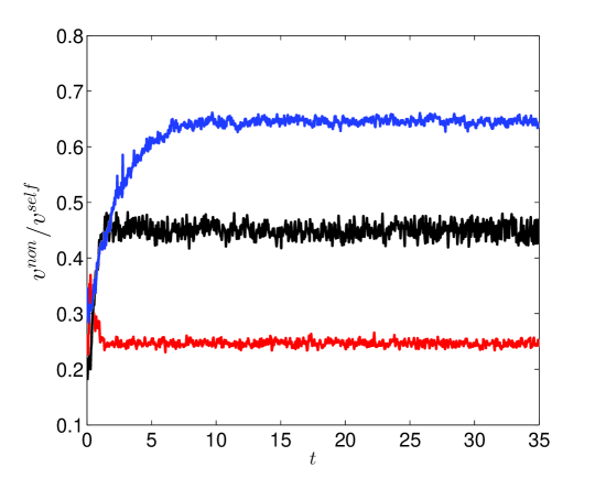
Figure 9: (color online). Ratio of nonlocal to total self-induced velocity as a function of time $t$ $\rm(s)$ for tangles generated by uniform normal fluid (model 1, red line, bottom), synthetic normal fluid turbulence (model 2, black line, middle) and frozen Navier-Stokes turbulence (model 3, blue line, top). Parameters as in Fig. (2).

The natural question which we ask is what is the cause of the spectral difference shown in Fig. 6. To answer the question we examine the local and nonlocal contributions to the superfluid velocity, defined according to Equation 4. Fig. 9 shows the fraction $v^{non}/v^{self}$ of the superfluid velocity which arises from nonlocal contributions, where $v^{non}=<|{\bf{v}}_{non}({\bf{s}}_{j})|>$ and $v^{self}=<|{\bf{v}}_{self}({\bf{s}}_{j})|>$ are sampled over the discretization points $j=1,\cdots N$ at a given time $t$. The difference is striking. Nonlocal effects are responsible for only 25 percent of the total superfluid velocity field in the tangle generated by the uniform normal fluid (model 1), for 45 percent in the tangle generated by synthetic normal flow turbulence (model 2), and for more than 60 percent in the tangle generated by frozen Navier-Stokes turbulence (model 3).

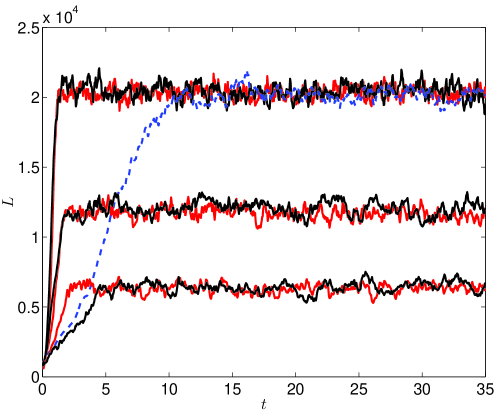
Figure 10: (color online). Evolution of the vortex line density $L$ (cm^-2) vs time $t$ (s) for model 1 (red line, uniform normal flow, respectively at $V_{n}=1~{}\rm(cm/s)$ (top), $V_{n}=0.75~{}\rm(cm/s)$ (middle) and $V_{n}=0.55~{}\rm(cm/s)$ (bottom)), model 2 (black line, synthetic normal fluid turbulence, respectively at $Re=79.44$ (top), $Re=81.59$ (middle) and $Re=83.86$ (bottom)), and model 3 (dashed blue line, frozen Navier-Stokes turbulence, at $Re=3025$).

Finally, we explore the dependence of the result on the vortex line density $L$ by generating statistically steady states of turbulence driven by uniform normal fluid (model 1) and synthetic turbulence (model 2) with different values of $L$, see Fig. 10. Fig. 11 shows that for model 1 (uniform normal flow) the relative importance of nonlocal contributions remains constant at about 25 percent over a wide range of vortex line density, from $L\approx 6000$ to $L\approx 20,000~{}{\rm cm^{-2}}$, whereas for model 2 (synthetic normal flow turbulence) and 3 (frozen Navier–Stokes turbulence), it increases with $L$.

IV Conclusion

Turbulent vortex tangles can be produced in the laboratory using various means: by imposing a flux of heat, by pushing liquid helium II through pipes, or by stirring it with moving objects. The numerical experiments presented here show that reporting the vortex line density $L$ is not enough to characterize the nature of the superfluid turbulence which can be generated in helium II. Vortex tangles with the same value of $L$ may have very different energy spectra, depending on the normal fluid flow which feeds energy into the vortex lines, as shown in Fig. 6. If the normal fluid is turbulent, energy is contained in the large eddies and is distributed over the length scales consistent with the classical $k^{-5/3}$ Kolmogorov law at large $k$, suggesting the presence of a Richardson cascade. If the normal fluid is uniform, most of the energy is contained at the intermediate length scales, and the energy spectrum scales consistently with $k^{-1}$ at large $k$. Using a terminology already in the literature, we identify these two forms of superfluid turbulence as ‘Kolmogorov tangles’ and ‘Vinen tangles’ respectively.

The superfluid velocity field is determined by the instantaneous configuration of vortex lines. Since the superfluid velocity field decays only as $1/r$ away from the axis of a quantum vortex line, the interaction between vortex lines is long-ranged, at least in principle. By examining the ratio of local and nonlocal contributions to the total velocity field, we have determined that in Vinen tangles far-field effects tend to cancel out ($v_{s}^{non}/v_{s}^{self}\approx 25\%$ independently of $L$), the motion of a vortex line is mainly determined by its local curvature, and the vortex tangle is homogeneous. In Kolmogorov tangles, on the contrary, nonlocal effects are dominant and increase with the vortex line density; this stronger vortex-vortex interaction leads to the clustering of vortex lines, for which the vortex tangle is much less homogeneous and contains coherent vorticity regions, in analogy to what happens in ordinary turbulence. The presence of intermittency effects such as coherent structures in the driving normal fluid, which we have explored with model 3, enhances the formation of superfluid vortex bundles, resulting in a more inhomogeneous superfluid energy and in larger nonlocal contributions to the vortex lines’ dynamics.

Future work will explore the problem for turbulence with nonzero mean flow.

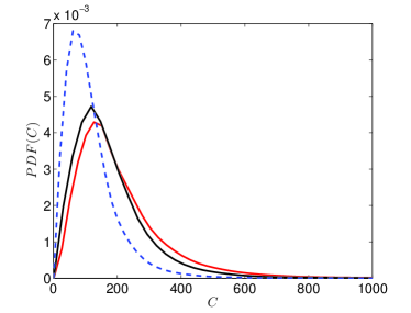
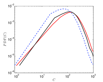
Figure 5: (color online). Left: Probability density function of the curvature, ${\rm PDF}(C)$, vs curvature, $C$ ($\rm cm^{-1}$), corresponding to model 1 (uniform normal flow, red line), model 2 (synthetic turbulence, black line) and model 3 (frozen Navier-Stokes turbulence, dashed blue line). Right: the same data plotted on a log log scale, where the matching slopes on the plot illustrate that we have the same Kelvin waves in all three models (because they are all at the same temperature). Parameters as in Fig. 2.

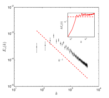
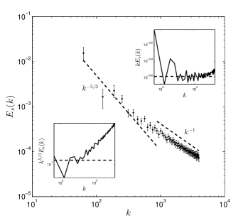
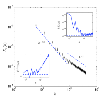
Figure 6: (color online). Energy spectrum $E(k)$ (arbitrary units) vs wavenumber $k$ ($\rm cm^{-1}$) (time averaged over the saturated regime) corresponding to vortex tangles generated by uniform normal fluid (model 1, top), synthetic normal fluid turbulence (model 2, middle) and frozen Navier-Stokes turbulence (model 3, bottom). The dashed lines indicate the $k^{-1}$ (top) and the $k^{-5/3}$ dependence (middle and bottom), respectively. Parameters as in Fig. (2). The compensated spectra $kE_{s}(k)$ and $k^{5/3}E_{s}(k)$ in the insets show the regions of $k$–space where the approximate scalings $k^{-1}$ and $k^{-5/3}$ apply.

- (1) R.J. Donnelly (1991) Quantized Vortices In Helium II (Cambridge University Press, Cambridge, UK).
- (2) C.F. Barenghi, L. Skrbek and K.R. Sreenivasan, Proc. Nat. Acad. Sci. USA 111, 4647 (2014).
- (3) S. Nemirovskii, Phys. Rep. 524 85 (2013)
- (4) W. F. Vinen and J. J. Niemela, J. Low Temp. Phys. 128, 167 (2002).
- (5) L. Skrbek and K.R. Sreenivasan, Phys. Fluids 24, 0113 (2012).
- (6) W.F. Vinen, Proc. R. Soc. A 240 114 (1957).
- (7) P.M. Walmsley and A.I. Golov, Phys. Rev. Lett. 100, 245301 (2008).
- (8) A.W. Baggaley, C.F. Barenghi, and Y.A. Sergeev, Phys. Rev. B 85, 060501 (2012).
- (9) G.E. Volovik J. Low Temp. Phys. 136, 309 (2004).
- (10) M.R. Smith, R.J. Donnelly, N. Goldenfeld, and W.F. Vinen, Phys. Rev. Lett. 71 2583 (1993).
- (11) J. Maurer, and P. Tabeling, Europhys. Lett. 43, 29 (1998).
- (12) J. Salort J, et al., Phys. Fluids 22, 125102 (2010).
- (13) A.W. Baggaley, L.K. Sherwin, C.F. Barenghi, and Y.A. Sergeev, Phys. Rev. B 86, 104501 (2012).
- (14) A.W. Baggaley, C.F. Barenghi, A. Shukurov, and Y.A. Sergeev, Europhys. Lett. 98, 26002 (2012).
- (15) A.W. Baggaley, J. Laurie, and C.F. Barenghi, Phys. Rev. Lett. 109, 205304 (2012).
- (16) U. Frisch, Turbulence. The legacy of A.N. Kolmogorov, Cambridge University Press, Cambridge (1995).
- (17) P.G. Saffman, Vortex Dynamics (Cambridge University Press, Cambridge (1992).
- (18) N.P. Proukakis and B. Jackson, J. Phys. B At. Mol. Opt. 40, 203002 (2008)
- (19) K.W. Schwarz, Phys. Rev. B 38, 2398 (1988).
- (20) K.W. Schwarz, Phys. Rev. B 31, 5782 (1985).
- (21) C. F. Barenghi, R. J. Donnelly, W. F. Vinen, J. Low Temp. Physics 52, 189 (1983).
- (22) R. J. Donnelly, C. F. Barenghi, J. Phys. Chem. Reference Data 27, 1217 (1998).
- (23) J. Koplik and H. Levine, Phys. Rev. Lett. 71, 1375 (1993).
- (24) G.P. Bewley, M.S. Paoletti, K.R. Sreenivasan, and D.P. Lathrop, Proc. Nat. Acad. Sci. USA 105, 13707 (2008).
- (25) S. Zuccher, M. Caliari, and C.F. Barenghi (2012), Phys. Fluids (24): 125108.
- (26) A.J. Allen, S. Zuccher, M. Caliari, N.P. Proukakis, N.G. Parker, and C.F. Barenghi, Phys. Rev. A 90, 013601 (2014).
- (27) A.W. Baggaley, J. Low Temp. Phys. 168, 18 (2012).
- (28) A.W. Baggaley, and C.F. Barenghi, Phys. Rev. E 84, 067301 (2011).
- (29) A.W. Baggaley and R. Hänninen, Proc. Nat. Acad. Sci. USA 111, 4667 (2014)
- (30) H. Adachi, S. Fujiyama, and M. Tsubota, Phys. Rev. B 81, 104511 (2010).
- (31) A.W. Baggaley and C.F. Barenghi, J. Low Temp. Phys. 66, 3 (2012).
- (32) D.R. Osborne, J.C. Vassilicos, K. Sung, and J.D. Haigh (2006), Phys. Rev. E 74, 036309 (2006).
- (33) The data set is available at the website turbulence.pha.jhu.edu
- (34) Y. Li, E. Perlman, M. Wan, Y. Yang, R. Burns, C. Meneveau, R. Burns, S. Chen, A. Szalay & G. Eyink. J. Turbulence 9, No. 31 (2008).
- (35) L.P. Kondaurova, V.A. Andryuschenko, and S.K. Nemirovskii, J. Low Temp. Phys. 150, 415 (2008).