Bouncing scalar field cosmology in the polymeric minisuperspace picture

Abstract

We study a cosmological setup consisting of a FRW metric as the background geometry with a massless scalar field in the framework of classical polymerization of a given dynamical system. To do this, we first introduce the polymeric representation of the quantum operators. We then extend the corresponding process to reach a transformation which maps any classical variable to its polymeric counterpart. It is shown that such a formalism has also an analogue in terms of the symplectic structure, i.e., instead of applying polymerization to the classical Hamiltonian to arrive its polymeric form, one can use a new set of variables in terms of which Hamiltonian retains its form but now the corresponding symplectic structure gets a new deformed functional form. We show that these two methods are equivalent and by applying of them to the scalar field FRW cosmology see that the resulting scale factor exhibits a bouncing behavior from a contraction phase to an expanding era. Since the replacing of the big bang singularity by a bouncing behavior is one of the most important predictions of the quantum cosmological theories, we may claim that our polymerized classical model brings with itself some signals from quantum theory.

PACS numbers: 04.60.Nc, 04.60.Kz
Keywords: Scalar field cosmology, Classical polymerization

1 Introduction

In the regimes that gravitational systems behave classically, general theory of relativity presents an almost complete description of such phenomena. Black hole physics and cosmology are perhaps the best examples which show the power of general relativity to explain how a system will be evolved under the act of gravity. However, it is well-known that there are also some aspects of these systems that general relativity fails to describe them. For example, we can refer to the problem of black hole radiation and all types of classical singularities that appear in the cosmological solutions to the Einstein field equations. Indeed, a quantum theory of cosmology is needed to understand the behavior of the universe in the vicinity of a classical singularity and also, the black hole radiation formalism is based on applying quantum field theory to the curved space-time around a black hole. Therefore, any hope of dealing with such issues would be in the development of a quantum theory of gravity which seems to be the main challenging task of theoretical physics and a wide variety of approaches are offered to the issue, from the DeWitt traditional canonical approach [1] to the more modern viewpoints of string theory and loop quantum gravity [2]-[4] in terms of which the space-time has a granular structure. The granularity property of the underlying space, in turn, supports the idea of existence of a minimal measurable length [5]-[8], one of the main features of which is to deform the algebraic structure of ordinary quantum mechanics.

One of the models that uses the idea of the existence of a minimal measurable length scale in its formalism is the so-called polymer quantization [9]. In this approach to quantization of a dynamical system one uses methods very similar to the effective models of loop quantum gravity [10]. In this scenario the main role is played by the polymer length scale in such a way that, unlike the deformed algebraic structure usually coming from the noncommutative phase-space variables, it enters into the Hamiltonian of the system to deform its functional form into a new one called the polymeric Hamiltonian. In the polymer representation of a quantum system the deformation parameter $\lambda$ in the Hamiltonian is responsible for the granularity property of the underlying space. The presence of this parameter is such that in the continuum limit when $\lambda\rightarrow 0$ the discrete geometry becomes continuum and the physical system behaves classically. Regards to this $\lambda$-dependent Hamiltonian, in the corresponding Hilbert space, the momentum operator is not defined by its normal way as in the usual quantum mechanics, instead it can be defined by a polymerization process in which the polymer scale comes into the play as a first-order parameter to define the derivative operator [9], [11]. With this motivations, polymer quantization has attracted some attentions in recent years in the fields which have to deal with the quantum gravitational effects in a physical system. Specially, in the domain of quantum features of cosmological models, it is shown that the $\lambda$-dependent classical cosmology leads to a modified Friedman equation which is very similar to the one that comes from loop quantization of the model [11]-[15].

Before going any further, some remarks are in order to clarify how the polymerization process, which originally is a quantum pattern, may work in a classical scheme. To see this, suppose a classical dynamical system is described by the Hamiltonian $H$. In the ordinary quantum version of this system the Hamiltonian operator contains the parameter $\hbar$ such that in the limit $\hbar\rightarrow 0$ the $\hbar$-dependent Hamiltonian $H_{\hbar}$ turns to its classical counterpart $H$. This is also true for the equations of motion, i.e., the classical equations of motion for the mentioned system are nothing but the $\hbar\rightarrow 0$ limit of the quantum dynamical equations. However, as we explain above, in the polymer picture of quantum mechanics the Hamiltonian operator $H_{\hbar,\lambda}$ gets an additional parameter $\lambda$, which is rooted in the ideas of minimum length. Now, note what happens if one deals with the classical limit $\hbar\rightarrow 0$ of this theory? It is clear that although the parameter $\hbar$ will disappear from the resulting classical Hamiltonian, this Hamiltonian is still labeled by the parameter $\lambda$. Therefore, we are facing with a classical theory that is not the one from which we begin and described by the Hamiltonian $H$, but a classical theory with a $\lambda$-dependent Hamiltonian $H_{\lambda}$. Of course, if all things are well arranged, we expect to recover the initial classical theory in the limit $\lambda\rightarrow 0$. It is believed that the solutions of such an (lets call them) effective classical theories can exhibit some important features of the corresponding dynamical system which may be related to quantum effects and more importantly, these effects can be achieved without quantization of the system. An excellent explanation of this process can be found in [16].

In this paper, after a brief review of a flat FRW cosmology in the presence of a massless scalar field, we introduce processes by means of which this setup can be polymerized. We show that this issue may be done by two equivalent methods. By one of them, to achieve a $\lambda$-deformed Hamiltonian, we define a transformation in phase-space which transforms the usual phase-space variables to their polymer counterparts and by another, we find a non-canonical coordinate transformation such that in terms of its new variables the Hamiltonian retains its functional form but the corresponding symplectic structure will be deformed. We then apply these two methods to the above mentioned scalar field cosmological model to arrive at the polymeric counterpart of the equations of motion. It is shown that although these two methods of polymerization give different equations of motion, the resulting scale factor and scalar field, as the solution of the equations of motion, have the same form independent of from which method they are obtained. We finally summarize the work by a discussion around the possible relation between the classical polymerization and quantum effects.

2 Scalar field cosmology: a brief review

In this section we consider the simplest dynamical model of space-time, compatible with the assumption of a flat, homogeneous and isotropic space on large scales. The geometry of such a space-time is described by the Friedmann-Robertson-Walker (FRW) metric with zero curvature index

$$ds^{2}=-N^{2}(t)dt^{2}+a^{2}(t)(dx^{2}+dy^{2}+dz^{2}),$$ (1)

where $N(t)$ is the lapse function and $a(t)$ denotes the scale factor which measures the expansion or contraction of the universe in terms of the time variable $t$. By definition of the cosmological proper time $\tau$ via $d\tau=Ndt$, the function $N(t)$ may be absorbed in time coordinate. Therefore, the above metric has only one dynamical variable $a(t)$. If we also consider a free scalar field $\phi(t)$ minimally coupled to the gravity, the dynamics of the total cosmological setting will be

$${\cal S}=\int d^{4}x\sqrt{-g}\left(\frac{1}{16\pi G}R-\frac{1}{2}g^{\mu\nu}\partial_{\mu}\phi\partial_{\nu}\phi\right),$$ (2)

in which we have used the notation $g$, $G$ and $R$ for the determinant of the metric tensor $g_{\mu\nu}$, Newton gravitational constant and the Ricci scalar respectively. The Einstein field equations for the gravitational field and also the scalar field Klein-Gordon equation can be obtained by variation of the above action with respect to $g_{\mu\nu}$ and $\phi$ respectively. However, in order to pass to the polymerized counterpart of the theory in the next section and compare the results, we prefer to obtain the dynamics from the Hamiltonian equations. The best way to do this issue is to follow the ADM formalism and express the action in terms of the minisuperspace variables $(a,\phi)$. By this method the Lagrangian (and hence the Hamiltonian) of the model (see relations (3) and (5) below) is very similar to the one of a point particle moving in a two dimensional space with coordinates $(a,\phi)$. So, by substituting the Ricci scalar associated with the metric (1), that is

$$R=6\left(\frac{\ddot{a}}{N^{2}a}+\frac{\dot{a}^{2}}{N^{2}a^{2}}-\frac{\dot{N}\dot{a}}{aN^{3}}\right),$$

and integration over spatial dimensions, we obtain a point-like Lagrangian as

$$L(a,\phi,\dot{a},\dot{\phi})=-\frac{3}{8\pi G}a\dot{a}^{2}+\frac{1}{2}a^{3}\dot{\phi}^{2},$$ (3)

in which we have set $N=1$ so that the time parameter $t$ is the usual cosmic time. The momenta conjugate to the variables $(a,\phi)$ can be calculated from their standard definition as

$$p_{a}=\frac{\partial L}{\partial\dot{a}}=-\frac{3}{4\pi G}a\dot{a},\hskip 14.22636ptp_{\phi}=\frac{\partial L}{\partial\dot{\phi}}=a^{3}\dot{\phi},$$ (4)

from which by the usual canonical analysis one derives the Hamiltonian

$$H=-\frac{2\pi G}{3}\frac{p_{a}^{2}}{a}+\frac{p_{\phi}^{2}}{2a^{3}},$$ (5)

which is constrained to vanish due to gauge freedom of the action. Now, we can write the classical dynamics from the Hamiltonian equations, that is

$$\left\{\begin{array}[]{ll}\dot{a}=\{a,H\}=-\frac{4\pi G}{3}\frac{p_{a}}{a},\\ \\ \dot{p_{a}}=\{p_{a},H\}=-\frac{2\pi G}{3}\frac{p_{a}^{2}}{a^{2}}+\frac{3p_{\phi}^{2}}{2a^{4}},\\ \\ \dot{\phi}=\{\phi,H\}=\frac{p_{\phi}}{a^{3}},\\ \\ \dot{p_{\phi}}=\{p_{\phi},H\}=0.\end{array}\right.$$ (13)

Since for a given cosmological setting, any solution of the Einstein field equations should satisfy the Hamiltonian constraint $H=0$, we may consider this condition as the first integral of the above field equations. So, with the help of (5) the Friedmann equation takes the form

$$a^{4}\dot{a}^{2}-\alpha^{2}=0,$$ (14)

where $\alpha^{2}=4\pi Gp_{0}^{2}/3$ and we take $p_{\phi}=p_{0}=\mbox{const.}$ from the last equation of (13). This equation can easily be integrated to obtain the scale factor as

$$a_{\pm}(t)=(\pm 3\alpha t-t_{0})^{1/3},$$ (15)

where $t_{0}$ is an integration constant. Assuming a positive value for $t_{0}$, the condition $a(t)\geq 0$ would indicate that the expressions of $a_{+}(t)$ and $a_{-}(t)$ are valid for $t\geq\tau_{0}$ and $t\leq-\tau_{0}$ respectively, where $\tau_{0}=t_{0}/3\alpha$. Therefore, by using of the third equation of the system (13), we get the complete set of the solution as

$$\left\{\begin{array}[]{ll}a_{-}(t)=(-3\alpha t-t_{0})^{1/3},\\ \\ \phi_{-}(t)=-\frac{p_{0}}{3\alpha}\ln(-3\alpha t-t_{0}),\end{array}\right.$$ (19)

for $t\leq-\tau_{0}$ and

$$\left\{\begin{array}[]{ll}a_{+}(t)=(3\alpha t-t_{0})^{1/3},\\ \\ \phi_{+}(t)=\frac{p_{0}}{3\alpha}\ln(3\alpha t-t_{0}),\end{array}\right.$$ (23)

for $t\geq\tau_{0}$. These equations show that the dynamical behavior of the universe with the scale factor $a_{+}(t)$ begins with a big-bang singularity at $t=\tau_{0}$ and then follows an expansion phase at late times of cosmic evolution. For a universe with the scale factor $a_{-}(t)$, on the other hand, the behavior is opposite. The universe decreases its size from large values of scale factor at $t=-\infty$ and ends its evolution at $t=-\tau_{0}$ with a zero size singularity. In figure 1 we have shown the above mentioned behaviors for these two sets of solution. It should be noted that although we know that the universe is now in an expansion phase, the contracting solution of the Einstein field equations are also mathematically acceptable. However, the expanding and contracting phases are disconnected from each other and should not consider as simultaneously solutions of the system of field equations, i.e., the expansionary phase will not occur after a contraction phase or vice versa. In the next section we will see how this picture may be modified if one enters the issues arising from an effective theory into the problem at hand.

Before going to the next section to see how the above picture of the classical model may be modified by means of the polymerization mechanism, we would like to take a look at the Lagrangian equations of motion correspond to the model. From (3) the Euler-Lagrange equations read as

$$\left\{\begin{array}[]{ll}\frac{d}{dt}\frac{\partial L}{\partial\dot{a}}-\frac{\partial L}{\partial a}=0\Rightarrow\dot{a}^{2}+2a\ddot{a}+4\pi Ga^{2}\dot{\phi}^{2}=0,\\ \\ \frac{d}{dt}\frac{\partial L}{\partial\dot{\phi}}-\frac{\partial L}{\partial\phi}=0\Rightarrow\frac{d}{dt}(a^{3}\dot{\phi})=0.\end{array}\right.$$ (27)

Combination of the above equations yields

$$a^{4}\dot{a}^{2}+2a^{5}\ddot{a}+3\alpha^{2}=0.$$ (28)

It is easy too check that our previously set of solutions (19) and (23) satisfy the Lagrangian equation of motion (28). However, with $a_{0}$ and $t_{0}$ being some integration constants and $\tau^{2}=9\alpha^{2}/4a_{0}^{6}$, this equation also admits the following solutions

$$\left\{\begin{array}[]{ll}a(t)=a_{0}\left[(t-t_{0})^{2}-\tau^{2}\right],\\ \\ \phi(t)=\phi_{0}\tanh^{-1}\frac{t-\tau}{t_{0}},\end{array}\right.$$ (32)

which seems to be another set of solutions for our problem at hand. But we should take care of that this solution does not satisfy the Hamiltonian constraint $H=0$, and in this sense cannot be considered as physical solution. Therefore, by the Lagrangian formalism we are led again to the same solutions as we have already obtained by the Hamiltonian equations of motion.

3 Classical polymerization

3.1 Polymeric transformation

We saw in the previous section how our classical model suffers from the presence of a past or future big-bang like singularity, which shows that some consequences may be physically unacceptable. It is believed that dealing with such singularities would be in the development of a quantum theory of gravity, according to which the space-time, when it is considered in the high energy limit, has a discrete structure due to the existence of natural cutoffs such as the minimal measurable length. In Schrödinger picture of quantum mechanics, one usually feels free to work in the alternative position or momentum space representations. However, in the presence of the quantum gravitational effects the space-time manifold may take a fuzzy structure so that the well-defined Schrödinger representations are no longer applicable [17]-[19]. One of the recently proposed quantum frameworks which considers a discrete nature for space in its formalism is the so-called polymer representation of quantum mechanics [9, 10]. Instead of the Hilbert space ${\mathcal{H}}=L^{2}(R,dq)$, in which the Schrödinger quantum mechanics is formulated (here $dq$ is the Lebesgue measure on the real line $R$), it is shown that the appropriate Hilbert space to formulate the polymer quantum mechanics is ${\mathcal{H}}_{\rm poly}=L^{2}(R_{{}_{d}},d\mu_{{}_{d}})$, where $d\mu_{{}_{d}}$ is the Haar measure, and $R_{{}_{d}}$ denotes the real line but now endowed with a discrete topology. The extra structure in polymer picture is properly described by a dimension-full parameter $\lambda$ such that the standard Schrödinger representation will be recovered in the continuum limit $\lambda\rightarrow\,0$ [9]. Evidently, the classical limit of the polymer representation $\hbar\rightarrow\,0$, does not yield to the classical theory from which one has started but to an effective $\lambda$-dependent classical theory which may be interpreted as a classical discrete theory. Such an effective theory can also be extracted directly from the standard classical theory (without any attribution to the polymer quantum picture) by using of the Weyl operator [16]. The process is known as polymerization with which we will deal in the rest of this paper.

In polymer representation of quantum mechanics, the position space (with coordinate $q$) is assumed to be discrete with discreteness parameter $\lambda$ and consequently the associated momentum operator $\hat{p}$, that would be a generator of the displacement, does not exist [10]. However, the Weyl exponential operator (shift operator) correspond to the discrete translation along $q$ is well defined and effectively plays the role of momentum for the system under consideration [9]. Taking this fact into account, one can utilize the Weyl operator to find an effective momentum in the semiclassical regime. Therefore, the derivative of the state $f(q)$ with respect to the discrete position $q$ can be approximated by means of the Weyl operator as [16]

$$\partial_{q}f(q)\approx\frac{1}{2\lambda}[f(q+\lambda)-f(q-\lambda)]\hskip 56.9055pt$$

$$=\frac{1}{2\lambda}\Big{(}\widehat{e^{ip\lambda}}-\widehat{e^{-ip\lambda}}\Big{)}\,f(q)=\frac{i}{\lambda}\widehat{\sin(\lambda p)}\,f(q),$$ (33)

and similarly the second derivative approximation gives

$$\partial_{q}^{2}f(q)\approx\frac{1}{\lambda^{2}}[f(q+\lambda)-2f(q)+f(q-\lambda)]\hskip 28.45274pt$$

$$=\frac{2}{\lambda^{2}}(\widehat{\cos(\lambda p)}-1)\,f(q).\hskip 56.9055pt$$ (34)

Inspired by the above approximations, the polymerization process is defined for the finite values of the parameter $\lambda$ as

$$\hat{p}\rightarrow\,\frac{1}{\lambda}\widehat{\sin(\lambda p)},\hskip 28.45274pt\hat{p}^{2}\rightarrow\,\frac{2}{\lambda^{2}}(1-\widehat{\cos(\lambda p)}).$$ (35)

This replacement suggests the idea that a classical theory may be obtained via this process that is dubbed usually as Polymerization in literature [9, 16]

$$q\rightarrow q,\hskip 42.67912ptp\rightarrow\frac{\sin(\lambda p)}{\lambda},\hskip 14.22636ptp^{2}\rightarrow\frac{2}{\lambda^{2}}\left[1-\cos(\lambda p)\right],$$ (36)

and in a same manner one can find polymer transformation of the higher powers of momentum $p$. In this sense, by a classical polymerized system, we mean a system that the transformation (36) is applied to its Hamiltonian. The first consequence of the polymerization (36) is that the momentum is periodic and its range should be bounded as $p\in[-\frac{\pi}{\lambda},+\frac{\pi}{\lambda})$. In the limit $\lambda\rightarrow\,0$, one recovers the usual range for the canonical momentum $p\in(-\infty,+\infty)$. Therefore, the polymerized momentum is compactified and topology of the momentum sector of the phase space is $S^{1}$ rather than the usual $R$ [20].

3.2 Polymeric symplectic structure

Now, let us take a look at the Hamiltonian formalism in the context of symplectic geometry. Given a configuration space ${\mathcal{Q}}$ of a dynamical system, the corresponding cotangent bundle $T^{\ast}{\mathcal{Q}}$ (phase space) is naturally a symplectic manifold endowed with a symplectic structure $\omega$ which, in turn, is a closed non-degenerate $2$-form. In a local coordinate $(q^{1},...,q^{n},p_{1},...,p_{n})$ on $T^{\ast}{\mathcal{Q}}$ the symplectic structure takes the canonical form

$$\omega=\sum_{i=1}^{n}dq^{i}\wedge dp_{i}\,,$$ (37)

where $(q^{i},p_{i})$ are called canonical variables. The evolution of the system is given by

$$i_{{}_{X_{H}}}\omega=dH.$$ (38)

Substituting of ${X_{H}}=\sum_{i=1}^{n}\big{(}\frac{{dq}^{i}}{dt}\frac{\partial}{\partial q^{i}}+\frac{{dp}_{i}}{dt}\frac{\partial}{\partial p_{i}})$ into the equation (38) with canonical structure (37), the standard Hamilton’s equations for $(q^{i}(t),p_{j}(t))$ are emerged that are the integral curves of $X_{H}$. For the minisuperspace $(q^{i},p_{j})=(a,\phi,p_{a},p_{\phi})$ we have considered in section 2, these are indeed the set of equations (13).

The triplet $(H,{\omega},X_{H})$ constitutes a Hamiltonian system. In order to study more complicated physical cases such as systems with a noncommutative or polymeric structure, the corresponding Hamiltonian system may includes some extra deformation parameters. Here, we are going to claim that there are two distinct but equivalent methods to enter the mentioned extra parameters into the scenario:

$\bullet$ Approach I: In the first method we modify the Hamiltonian to get a deformed Hamiltonian $H_{\lambda}$ where $\lambda$ is the deformation parameter. In this method one does not change the symplectic structure, so that the equations of motion can be constructed as the usual case but now with the new Hamiltonian $H_{\lambda}$. In the polymeric systems, for instance, this method will be done by applying the polymerization transformation (36) on the Hamiltonian. In this sense, in a two dimensional phase space a typical Hamiltonian $H(q,p)=p^{2}/2m+U(q)$ takes the form

$$H_{{}_{\lambda}}=\frac{1}{m\lambda^{2}}\left[1-\cos(\lambda p)\right]+U(q),$$ (39)

with the use of which and the canonical symplectic structure $\omega=dq\wedge dp$ in relation (38) one is led to the Hamilton’s equations of motion $\dot{q}=\sin(\lambda p)/m\lambda$ and $\dot{p}=-\partial U/\partial q$.

$\bullet$ Approach II: In the second method, we seek a new set of variables in terms of which the Hamiltonian takes its non-deformed form. What is modified in this method is the symplectic structure $\omega$ according to which the deformation parameter shows itself in the equations of motion. To clarify this method in the polymer framework, let us consider again the above two dimensional case and apply the following non-canonical transformation on its polymeric phase space $\Gamma_{\lambda}$

$$(q,p)\rightarrow\,(q^{\prime},p^{\prime})=\Big{(}q,\frac{2}{\lambda}\sin(\frac{\lambda p}{2})\Big{)},$$ (40)

under the act of which the polymeric Hamiltonian (39) becomes $H=\frac{p^{\prime 2}}{2m}+U(q^{\prime})$ and the corresponding symplectic 2-form will be

$$\omega_{{}_{\lambda}}=\frac{dq^{\prime}\wedge\,dp^{\prime}}{\sqrt{1-(\lambda p^{\prime}/2)^{2}}}\,.$$ (41)

Since the canonical momentum $p$ varies in a bounded domain, according to transformation (40) the range of the new momentum $p^{\prime}$ should be also bounded as $[-\frac{2}{\lambda},+\frac{2}{\lambda})$. Also, the new 2-form symplectic structure $\omega_{{}_{\lambda}}$ does not have the canonical form and therefore the variables $(q^{\prime},p^{\prime})$ should be considered as a pair of non-canonical variables. By means of this set-up equation (38) gives the associated Hamiltonian vector field $X_{H}$ whose integral curves may be written as $\dot{q^{\prime}}=\frac{p^{\prime}}{m}\,\sqrt{1-(\lambda p^{\prime}/2)^{2}}$ and $\dot{p^{\prime}}=-\frac{\partial U}{\partial q^{\prime}}\,\sqrt{1-(\lambda p^{\prime}/2)^{2}}$.

With a straightforward calculation based on the transformation (40) it is easy to show that the resulting dynamics is the same regardless of whether it is obtained from the first or the second approach. This means that by dealing either with $(\omega_{\lambda},H)$ or with $(\omega,H_{\lambda})$ one leads to the same $X_{H}$. This issue may be understood from the fact that equation (38) which defines $X_{H}$ is written in a coordinate independent manner. Therefore, although $X_{H}$ has different components when it is represented in terms of different coordinates $(q,p)$ or $(q^{\prime},p^{\prime})$ that are related to each other by (40), as a geometrical object, $X_{H}$ has an unique character independent of these coordinates. In the next section we will apply the above mentioned classical polymerization formalism to the scalar field cosmological model described in section 2.

4 Scalar field cosmology: polymeric dynamics

In this section let us examine how the scalar field cosmological setting in section 2 may change with polymeric considerations. As we saw in section 2 this model has a four dimensional phase space whose coordinates are $(a,\phi,p_{a},p_{\phi})$ and its dynamics is given by Hamiltonian (5). It is important to note that we only polymerize the geometrical part of the minisuperspace, that is $(a,p_{a})$, while the matter part $(\phi,p_{\phi})$ does not contribute to our polymerization process [16]. Therefore, polymerization of this system according to the approach (I), will lead us the effective Hamiltonian

$$H_{\lambda}=-\frac{4\pi G}{3\lambda^{2}a}\left[1-\cos(\lambda p_{a})\right]+\frac{p_{\phi}^{2}}{2a^{3}}=-\frac{8\pi G}{3\lambda^{2}a}\sin^{2}(\frac{\lambda p_{a}}{2})+\frac{p_{\phi}^{2}}{2a^{3}},$$ (42)

and the canonical symplectic structure

$$\omega=da\wedge dp_{a}+d\phi\wedge dp_{\phi}.$$ (43)

Now, equation (38) with

$$X_{H}=\frac{da}{dt}\frac{\partial}{\partial a}+\frac{{dp_{a}}}{dt}\frac{\partial}{\partial p_{a}}+\frac{{d\phi}}{dt}\frac{\partial}{\partial\phi}+\frac{{dp_{\phi}}}{dt}\frac{\partial}{\partial p_{\phi}},$$ (44)

yields the following equations of motion

$$\left\{\begin{array}[]{ll}\dot{a}=-\frac{4\pi G}{3\lambda a}\sin(\lambda p_{a}),\\ \\ \dot{p_{a}}=-\frac{8\pi G}{3\lambda^{2}a^{2}}\sin^{2}(\frac{\lambda p_{a}}{2})+\frac{3p_{\phi}^{2}}{2a^{4}},\\ \\ \dot{\phi}=\frac{p_{\phi}}{a^{3}},\\ \\ \dot{p_{\phi}}=0.\end{array}\right.$$ (52)

On the other hand if we go ahead through the approach (II), our starting point will be the non-deformed Hamiltonian (5) but now with the polymeric structure

$$\omega_{{}_{\lambda}}=\frac{da\wedge\,dp_{a}}{\sqrt{1-(\lambda p_{a}/2)^{2}}}+d\phi\wedge dp_{\phi},$$ (53)

which is obtained in the light of the deformed symplectic structure (41). Clearly the matter part of the symplectic 2-form is remained unchanged since the polymerization only acts on the geometrical part of the minisuperspace. Substituting the Hamiltonian (5) and polymeric symplectic structure (41) together with the Hamiltonian vector field (44) into the relation (38) gives the following equation of motion for the triplet $(H,\omega_{\lambda},X_{H})$

$$\left\{\begin{array}[]{ll}\dot{a}=-\frac{4\pi G}{3}\frac{p_{a}}{a}\sqrt{1-(\frac{\lambda p_{a}}{2})^{2}},\\ \\ \dot{p_{a}}=-\frac{2\pi G}{3}(\frac{p_{a}}{a})^{2}+\frac{3}{2}\frac{p_{\phi}^{2}}{a^{4}},\\ \\ \dot{\phi}=\frac{p_{\phi}}{a^{3}},\\ \\ \dot{p_{\phi}}=0.\end{array}\right.$$ (61)

From the first equation of this system we have

$$\dot{a}^{2}=\frac{16\pi^{2}G^{2}p_{a}^{2}}{9a^{2}}\Big{(}1-(\frac{\lambda p_{a}}{2})^{2}\Big{)},$$ (62)

which upon substitution the expression $p_{a}^{2}=\frac{3p_{\phi}^{2}}{4\pi Ga^{2}}$, from the constraint equation $H=0$ one gets

$$\dot{a}^{2}=\frac{4\pi Gp_{\phi}^{2}}{3a^{4}}\Big{(}1-\frac{3\lambda^{2}p_{\phi}^{2}}{16\pi Ga^{2}}\Big{)}.$$ (63)

It is easy to show that this equation can also be extracted from the system (52) with the help of the constraint equation $H_{\lambda}=0$. Taking into account from the last equation of (61) that $p_{\phi}=p_{0}=\mbox{cons.}$, the above equation will be casted into the form

$$a^{3}\dot{a}=\pm\alpha\sqrt{a^{2}-\beta^{2}},$$ (64)

where $\alpha^{2}=4\pi Gp_{0}^{2}/3$ and $\beta^{2}=3\lambda^{2}p_{0}^{2}/16\pi G$. This equation can be integrated to yield the solution

$$a_{\lambda}^{\pm}(t)=\bigg{\{}-\beta^{2}+\frac{2^{1/3}\beta^{4}}{\left[2\beta^{6}+(\pm 3\alpha t-t_{0})^{2}+(\pm 3\alpha t-t_{0})\sqrt{4\beta^{6}+(\pm 3\alpha t-t_{0})^{2}}\right]^{1/3}}+$$

$$\frac{1}{2^{1/3}}\left[2\beta^{6}+(\pm 3\alpha t-t_{0})^{2}+(\pm 3\alpha t-t_{0})\sqrt{4\beta^{6}+(\pm 3\alpha t-t_{0})^{2}}\right]^{1/3}\bigg{\}}^{1/2},$$ (65)

where $t_{0}$ is an integration constant. This expression provides a classical description of the scale factor as modified by effective polymer dynamics. At the first glance it may seem that it differs from the classical scale factor obtained in section 2 by a complex relation. However, by a deeper look we realize that it satisfies all of our expectations from a polymeric theory. First, it is seen that in the limit $\lambda\rightarrow 0$ the above expression takes the form of the ordinary case given in (15). Second, due to the presence of the parameter $\lambda$ in (4), it escapes from the classical scale factor only in the region where the scale factor tends to zero and for the large values of scale factor coincides on it (see also figure 1 and discussion below). To evaluate the dynamics of the scalar field, it is better to expand $a_{\lambda}(t)$ as

$$a_{\lambda}^{\pm}(t)\sim(\pm 3\alpha t-t_{0})^{1/3}-\frac{\beta^{2}}{2(\pm 3\alpha t-t_{0})^{1/3}}+O(\beta^{3}),$$ (66)

so that from the third equation of the system (52) one obtains

$$\phi_{\lambda}^{\pm}(t)=\frac{p_{0}}{\alpha}\left[\pm\frac{1}{3}\ln\left(\pm 3\alpha t-t_{0}\right)-\frac{3}{4}\frac{\beta^{2}}{\left(\pm 3\alpha t-t_{0}\right)^{2/3}}+O(\beta^{3})\right].$$ (67)

Now, let’s see how the polymeric picture might lead to a resolution of the primordial singularity appeared in the results of section 2 and yields instead a bouncing connexion between contracting and expanding phases. In figure 1 the scale factors are plotted together with their non-deformed counterparts. In section 2 we have seen that the corresponding scalar field classical cosmology admits two separate solutions, which are disconnected from each other by a classically forbidden region. One of these solutions represents a contracting universe ending in a singularity while another describes an expanding universe which begins its evolution with a big bang singularity. As this figure shows in the case where the classical model is polymerized, the scale factor has a bouncing behavior, i.e. the expansion phase in the cosmic evolution is followed by a contraction phase. In this picture the classically forbidden region is where the universe bounces from a contraction epoch to a re-expansion era. It is clear that the reason for the bouncing behavior in the vicinity of the classical singularity is the existence of the $\lambda$-term in the polymeric model. Therefore, if we consider the bouncing point as the minimum size of the universe as suggested by quantum theories of cosmology, our polymerization process support the idea that the polymeric corrections to the classical cosmology are some signals from quantum gravity.

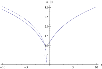
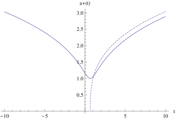
Figure 1: Qualitative behavior of the scale factors versus time based on relation 15 (dashed lines) and 4 (solid lines).

5 Summary

In this letter we have studied the possibility of removing the big bang singularity from a scalar field model of FRW cosmology by introducing a classical process called polymerization. For this purpose, we first reviewed a flat FRW geometry coupled to a massless scalar field as a simple cosmological model which exhibits big bang like singularity in its solutions. We have shown that this setup admits two separate sets of solutions, while one of them is an expanding universe begins its evolution from a big bang singularity, the scale factor of another decreases its size from large values until it eventually reaches a zero size singularity. These two sets are separated from each other by a classically forbidden time interval. Inspired by the polymer representation of quantum mechanics, we then have dealt with a deformed classical theory in which the momenta are transformed like their operator counterparts in polymer quantum mechanics. We also presented an alternative method to classically polymerized of the system, this time not by changing the functional form of the momenta and therefore the Hamiltonian, but by deforming the symplectic structure associated to the corresponding Hamiltonian system. Finally, we applied classical polymerization to the our minisuperspace model and solved the resulting equations of motion once again. Interestingly, we found that the scale factor displays a bouncing behavior, i.e., after a period of contraction, an expansion era occurs. In the late time of cosmic evolution the classical and the polymerized solutions will coincide to each other. However, when the classical solutions approaches their singularities the polymerized solutions get away from them and bounce from a minimum value the size of which is directly related to the polymeric deformation parameter. Bearing in the mind that the prediction of such a bouncing behavior for the scale factor is the main character of the quantum cosmological models, we conclude that the classical polymeric structure which we have constructed has a good correlation with quantum cosmology.

References

- [1] B.S. De Witt, Phys. Rev. 160 (1967) 1113
- [2] C. Rovelli and L. Smolin, Nucl. Phys. B 442 (1995) 593
- [3] A. Ashtekar and J. Lewandowski, Class. Quantum Grav. 14 (1997) A55
- [4] C. Rovelli, Living Rev. Rel. 1 (1998) 1
- [5] D.J. Gross and P.F. Mende, Nucl. Phys. B 303 (1988) 407
- [6] C.M. Ho, T.W. Kephart, D. Minic, Y.J. Ng, Mod. Phys. Lett. A 28 (2013) 1350005 (arXiv:1206.0085 [hep-th])
- [7] D. Amati, M. Ciafaloni and G. Veneziano, Phys. Lett. B 216 (1989) 41
- [8] L. Garay, Int. J. Mod. Phys. A 10 (1995) 145 (arXiv: gr-qc/9403008)
- [9] A. Corichi, T. Vukašinac and J.A. Zapata, Phys. Rev. D 76 (2007) 044016 (arXiv: 0704.0007 [gr-qc])
- [10] A. Ashtekar, S. Fairhurst and J. Willis, Class. Quantum Grav. 20 (2003) 1031 (arXiv: gr-qc/0207106)
- [11] M. Campiglia, Polymer representations and geometric quantization (arXiv: 1111.0638 [gr-qc])
- [12] G. De Risi, R. Maartens and P. Singh, Phys. Rev. D 76 (2007) 103531 (arXiv: 0706.3586 [hep-th])
- [13] V. Taveras, Phys. Rev. D 78, (2008) 064072 (arXiv: 0807.3325 [gr-qc])
- [14] G.M. Hossain, V. Husain and S.S. Seahra, Phys. Rev. D 81 (2010) 024005 (arXiv: 0906.2798 [astro-ph])
- [15] A. Corichi and A. Karami, Phys. Rev. D 84 (2011) 044003 (arXiv: 1105.3724 [gr-qc])
- [16] A. Corichi and T. Vukašinac, Phys. Rev. D 86 (2012) 064019 (arXiv: 1202.1846 [gr-qc])
- [17] A. Kempf, G. Mangano and R.B. Mann, Phys. Rev. D 52 (1995) 1108 (arXiv: hep-th/9412167)
- [18] H. Hinrichsen and A. Kempf, J. Math. Phys. 37 (1996) 2121
- [19] S. Hossenfelder, Living Rev. Rel. 16 (2013) 2 (arXiv: 1203.6191 [gr-qc])
- [20] K. Nozari, M. A. Gorji, V. Hosseinzadeh and B. Vakili, Natural Cutoffs via Compact Symplectic Manifolds (arXiv: 1405.4083 [gr-qc])