Nuclear inputs of key iron isotopes for core-collapse modeling and simulation

Abstract

From the modeling and simulation results of presupernova evolution of massive stars, it was found that isotopes of iron, ^54,55,56Fe, play a significant role inside the stellar cores, primarily decreasing the electron-to-baryon ratio ($Y_{e}$) mainly via electron capture processes thereby reducing the pressure support. The neutrinos produced, as a result of these capture processes, are transparent to the stellar matter and assist in cooling the core thereby reducing the entropy. The structure of the presupernova star is altered both by the changes in $Y_{e}$ and the entropy of the core material. Here we present the microscopic calculation of Gamow-Teller strength distributions for isotopes of iron. The calculation is also compared with other theoretical models and experimental data. Presented also are stellar electron capture rates and associated neutrino cooling rates, due to isotopes of iron, in a form suitable for simulation and modeling codes. It is hoped that the nuclear inputs presented here should assist core-collapse simulators in the process of fine-tuning of the $Y_{e}$ parameter during various phases of presupernova evolution of massive stars. A reliable and accurate time evolution of this parameter is a possible key to generate a successful explosion in modeling of core-collapse supernovae.

1 Introduction

The understanding of production of energy and matter in stars have come a long way since the seminal paper by Bethe [1]. Almost half a century later Bethe again tried to summarize the mechanisms of supernova explosions [2]. Today we know that there are two key quantities that control the complex dynamics of core-collapse supernovae: the lepton-to-baryon fraction ($Y_{e}$) and the core entropy. It is the weak-interaction rates (mainly electron capture and $\beta$-decay) that alter $Y_{e}$ and hence control the time evolution of this key parameter. At the same time the (anti)neutrinos produced by these weak rates are transparent to stellar matter for densities less than around 10¹¹ gcm^-3 and helps in removing energy and entropy from the stellar core.

Nuclei in the mass range A $\sim$ 60, at stellar densities less than around 10¹¹ gcm^-3, posses electron chemical potential of the same order of magnitude as the nuclear Q-value. Under such conditions the electron capture rates are sensitive to the detailed Gamow-Teller (GT) distributions. A reliable and microscopic calculation of ground and excited states GT distribution functions is then in order. Further to this, electron capture rates and associated neutrino cooling rates (as a function of stellar temperature, density and Fermi energy) are required by core-collapse simulators for modeling the dynamics and supernova collapse phase of massive stars (e.g. see the review article by Strother and Bauer [3]).

Isotopes of iron (mainly ^54,55,56Fe) play an effective role in the presupernova evolution of massive stars (see for example the simulation results of Refs. [4, 5]). The microscopic calculation of weak rates of these isotopes of iron was calculated by Nabi [6]. Later a detailed analysis of stellar electron capture rates [7] and neutrino cooling rates [8] on these iron isotopes were presented by the same author (see also [9, 10]). Keeping in view the paramount importance of weak rates of these iron isotopes in modeling and simulation of core-collapse supernovae, we present, in this paper, a detailed analysis of GT strength distributions as well as electron capture and neutrino cooling rates due to ^54,55,56Fe suitable for incorporation in stellar codes. The pn-QRPA model, first developed by Halbleib and Sorensen [11], and extended to nuclear excited states by Muto and collaborators [12], was used to calculate the ground and excited states GT strength distribution functions and stellar electron capture and neutrino cooling rates in a form suitable for use in modeling and simulation codes of core-collapse supernovae. Wherever possible we also compare and contrast our calculation with experiments and previous theoretical calculations. It is expected that the present work can assist in fine-tuning of the temporal variation of $Y_{e}$ parameter which is a key to generation of a successful explosion in modeling and simulation of core-collapse supernovae.

We present our calculation and results in next section and summarize the main conclusions in Section 3.

2 Calculations and Results

Calculation of electron capture (ec) and neutrino cooling rates ($\nu$) in stellar matter is given by

$$\lambda^{{}^{ec(\nu)}}_{ij}=\left[\frac{\ln 2}{D}\right]\left[f_{ij}^{ec(\nu)}(T,\rho,E_{f})\right]\left[B(F)_{ij}+\left({\raise 3.01385pt\hbox{$g_{A}$}\!\mathord{\left/{\vphantom{g_{A}g_{V}}}\right.\kern-1.2pt}\!\lower 3.01385pt\hbox{$g_{V}$}}\right)^{2}_{eff}B(GT)_{ij}\right].$$ (1)

The calculation of Fermi and GT reduced transition probabilities (within the pn-QRPA formalism) and phase space integrals in Eqt. 1 are not shown here because of space limitations and can be seen from Ref. [13]. A quenching factor of 0.6 was introduced in the calculation [6]. The value of D was taken as 6295 s.

The total electron capture (neutrino cooling) rate per unit time per nucleus is given by

$$\lambda^{ec(\nu)}=\sum_{ij}P_{i}\lambda_{ij}^{ec(\nu)},$$ (2)

where it is to be noted that $\lambda_{ij}^{\nu}$ contains contribution from both electron capture and positron decay rates for the transition $i$ (parent excited state) $\rightarrow j$ (daughter excited state) and $P_{i}$ is the probability of occupation of parent excited state which follows the normal Boltzmann distribution.

We next present the calculation of GT strength distribution functions within the pn-QRPA formalism which is later used to calculate the stellar electron capture and neutrino cooling rates. Wherever available, we also compare and contrast our calculation with measured data and previous theoretical calculations.

The pn-QRPA calculated GT strength values along the electron capture direction, B(GT₊), for ⁵⁴Fe are given in Table 1. We also present B(GT₊) distributions calculated using other pn-RPA scenarios for mutual comparison in Table 1 (adapted from Ref. [14]). The first three columns show calculated strength distributions using semi-realistic/semi-empirical shell model interactions. All three interactions started from realistic nucleon-nucleon interactions, from which an effective interaction (e.g., a G-matrix) was derived. The three interactions are similar, but have different starting points and were fitted to different data sets, with the following semi-realistic/semi-empirical interactions: the modified Kuo-Brown interaction KB3G [15], the Tokyo interaction GXPF1 [16] and the Brown-Richter interaction FPD6 [17]. For further details on these interactions we refer to Ref. [14]. The pn-QRPA calculated B(GT₊) values are given in fourth column. It is to be noted that calculated values of B(GT₊) of magnitude less than 10^-3 are not shown in Table 1 for space consideration. The pn-QRPA model calculates GT transitions at low excitation energy as against other three shell model interactions. It is further noted that the pn-QRPA calculated distribution is better fragmented than other RPA models and follows the trend of the measured data, albeit with a much higher magnitude of strength distribution. The measured data is shown in last column and is adapted from the ⁵⁴Fe(n,p) reaction, measured at 97 MeV for excitation energies in ⁵⁴Mn [18], and follows a more or less normal distribution till 8.5 MeV in ⁵⁴Mn. The fragmented data of pn-QRPA model is attributed to an optimum choice of particle-particle and particle-hole GT strength interaction parameters discussed later (for details see Ref. [10]).

Table 2 shows a similar calculated B(GT₊) distribution for ⁵⁵Fe. Once again calculated values of B(GT₊) of magnitude less than 10^-3 are not shown in Table 2 to save space. No experimental data is available for comparison for this odd-A nucleus of iron. Here one notes that the pn-QRPA model calculates high-lying transitions in daughter nucleus. Further the model calculates GT strength function up to around 14 MeV in ⁵⁵Mn. For ⁵⁵Fe nucleus, the excited states within the pn-QRPA formalism can be constructed:
(1) by lifting the odd neutron from ground state to excited states (one-quasiparticle state),
(2) by three-neutron states, corresponding to excitation of a neutron (three-quasiparticle states), or,
(3) by one-neutron two-proton states, corresponding to excitation of a proton (three-quasiparticle states).
The formulae for reduction of three-quasiparticle states to correlated one-quasiparticle state can be seen from Ref. [19]. The KB3G interaction saturates first to its maximum strength and also gives the lowest values for the centroid of the B(GT₊) distribution function.

The calculated and measured B(GT₊) distributions for ⁵⁶Fe are presented in Table 3. Calculated values of B(GT₊) of magnitude less than 10^-3 are not shown in Table 3 for space consideration. One notes that, akin to the case of ⁵⁴Fe, , the pn-QRPA model calculates low-lying GT strengths (as also measured in the experiment [20]). The calculated peak around 4 MeV in the pn-QRPA model takes care of low-lying measured data. It is easily seen from Table 3 that the pn-QRPA best mimics the trend in the measured GT data and is a triumph of the pn-QRPA model.

The key statistics of calculated GT strength distributions for ^54,55,56Fe is presented in Table 4. For the sake of completeness we present the data of GT distributions both in electron capture and in $\beta$-decay directions. We present the centroid E(GT), width and total GT strength for both electron capture and $\beta$-decay directions. Centroids and widths are given in units of MeV and B(GT) strengths are given in units such that B(GT) = 3 for neutron decay. The centroids and widths were calculated from the reported measured data and all measured data are given to one decimal place in Table 4. For the $\beta^{-}$ side the measured data for ⁵⁴Fe were taken from Refs. [21, 22, 23, 24]. For the electron capture direction, experimental data for ⁵⁴Fe were taken from Refs. [18, 21]. Measured data for ⁵⁶Fe in the electron capture direction were taken from Refs. [18, 20] while for the $\beta^{-}$ direction we only quote the reported value of $\sum B(GT_{-})$ = 9.9 $\pm$ 2.4 by Rapaport and collaborators [23]. The authors were unable to extract GT strengths for discrete excited states beyond 5.9 MeV in ⁵⁶Co making it impossible for us to calculate the centroid and width in this case. It is to be noted that we used a quenching factor of 0.6 for the calculated GT strength using the pn-QRPA model [7]. Note that the shell model interactions calculated strengths were quenched by a universal quenching factor of 0.55 rather than 0.6 (see [14]). Table 4 shows that the pn-QRPA model calculates the centroid at a much lower energy than other shell model interactions for ^54,56Fe and ⁵⁵Fe (along $\beta^{-}$ direction). Further in all cases it is seen that the pn-QRPA model best reproduces the placement of measured centroid. The comparison is exceptionally good for the case of GT_- centroid of ⁵⁴Fe and for the GT₊ centroids of ⁵⁶Fe. On the other hand the GXPF1 interaction calculates the highest centroid in daughter nuclei. Comparison of pn-QRPA calculated total GT strength with measured data is also reasonable. One should also keep in mind the uncertainties present in measurements as well as slightly different values of quenching factor used in pn-QRPA and shell model interactions before comparing the calculated numbers with experimental data. Table 4 shows that the pn-QRPA indeed is a good model for calculation of GT strength distribution for isotopes of iron. The pn-QRPA calculated GT strength distributions are in decent comparison with measurements and should therefore translate into a reliable calculation of stellar electron capture and neutrino cooling rates which we present below.

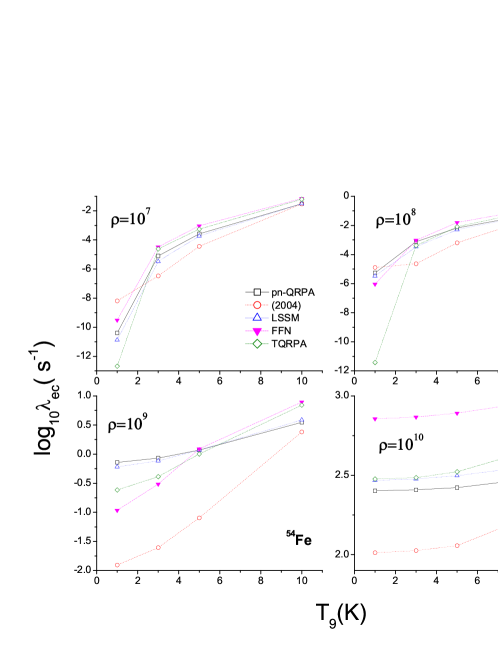
Figure 1: Comparison of electron capture rates on ⁵⁴Fe using current pn-QRPA model (pn-QRPA), previous pn-QRPA calculation (2004) [13], shell model calculation (LSSM) [25], calculation done by Ref. [26] (FFN) and calculation by Ref. [27] (TQRPA) at different selected stellar temperature and density zones.

We first present the calculation of stellar electron capture rates and also compare them with previous theoretical calculations. Fig. 1 shows a four-panel graph depicting the electron capture rates on ⁵⁴Fe. The upper left, upper right, lower left and lower right panels show electron capture rates calculated at stellar densities of 10⁷, 10⁸, 10⁹ and 10¹⁰ gcm^-3, respectively. T₉ gives stellar temperature in units of 10⁹ K. All electron capture rates are depicted in logarithmic scale (to base 10) and calculated in units of $s^{-1}$. The temperature and density zone selected for ⁵⁴Fe is pertinent for presupernova evolution of massive stars as per simulation results of Heger and collaborators [4]. In each panel we compare our results with four previous calculations: (i) previous pn-QRPA calculation of Nabi and Klapdor-Kleingrothaus [13] (2004); (ii) large scale shell model calculation [25] (LSSM); (iii) the pioneer weak-interaction mediated rate calculations performed by Fuller, Fowler and Newman [26] (FFN), and (iv) the pn-QRPA model extended to finite temperature using the thermofield dynamics formalism by Dzhioev and collaborators [27] (TQRPA). Details of other theoretical calculations can be found in the respective references. It can be noted from upper left panel of Fig. 1 that at a stellar density of 10⁷ gcm^-3 and T₉ =1, the current pn-QRPA calculation is around 3 orders of magnitude smaller than the previous pn-QRPA calculation of 2004 [13]. The two calculations get in better agreement at higher temperatures and densities. The difference arises because of a better choice of model parameters in current pn-QRPA calculation. In the current pn-QRPA model we took the values of $\chi$ (particle-hole GT strength parameter) and $\kappa$ (particle-particle GT strength parameter) as 0.15 MeV and 0.07 MeV, respectively. The values of these crucial parameters were different in previous pn-QRPA calculation. For a judicious selection of these GT strength parameters we refer to [10]. The deformation parameter is recently argued to be one of the most important parameters in pn-QRPA calculations [28] and as such rather than using deformations calculated from some theoretical mass model (as used in previous pn-QRPA calculation) the experimentally adopted value of the deformation parameters for ^54,56Fe, extracted by relating the measured energy of the first $2^{+}$ excited state with the quadrupole deformation, was taken from Raman et al. [29]. The incorporation of experimental deformations lead to an overall improvement in the calculation as discussed earlier in Ref. [19]. Our calculation is in overall very good agreement with LSSM results and around one order of magnitude smaller than corresponding FFN numbers. However it is to be noted that at T₉ =1, the reported electron capture rates on ⁵⁴Fe is around a factor three bigger than LSSM rates. The TQRPA electron capture rates are suppressed by around two orders of magnitude at T₉ =1. The comparison improves as temperature and density increase and TQRPA rates are doubled at T₉ =10. It appears that TQRPA rates are too sensitive to temperature changes. Moving to upper right panel (stellar density of 10⁸ gcm^-3) one notes that all calculations are within an order of magnitude differences except the TQRPA results which are around six orders of magnitude smaller at T₉ =1 than the reported rates. The two lower panels (stellar densities of 10^9,10 gcm^-3) also depict calculated rates which are within an order of magnitude differences of one another. The bigger electron capture rates on ⁵⁴Fe as calculated by FFN are due to the fact that FFN did not take into effect the process of particle emission from excited states and their parent excitation energies extended well beyond the particle decay channel. These high lying excited states begin to show their contribution to the total electron capture rate specially at high temperatures and densities. It is also to be noted that FFN neglected the quenching of the total GT strength in calculation of their stellar electron capture rates. Fig. 1 shows the fact that all calculations get in better agreement with each other at high densities whereas noticeable differences are seen at low temperature and densities.

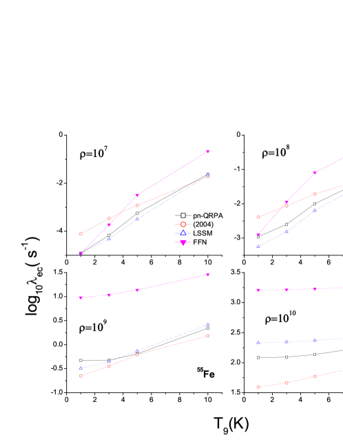
Figure 2: Same as Figure 1 but for ⁵⁵Fe. TQRPA model was not used to calculate electron capture rates on ⁵⁵Fe.

A similar comparison of electron capture rate calculations on ⁵⁵Fe is shown in Fig. 2. TQRPA formalism was not used to calculate electron capture rates on this odd-A isotope of iron and as such not present in Fig. 2. At stellar density of around 10⁷ gcm^-3 (upper left panel), one notes that reported electron capture rates are roughly an order of magnitude smaller as compared to previous pn-QRPA calculation. Only at T₉ =10 do the two calculations come in agreement. The reason for this difference was already discussed above. The comparison with FFN calculation is in reverse order. Here FFN calculated electron capture rates are in good agreement with reported rates at T₉ =1 and at all higher temperatures the reported rates are smaller by an order of magnitude. Once again the comparison with LSSM rates is excellent and speaks for the success of the pn-QRPA model. The comparison between different theoretical models remains more or less same at stellar density of 10⁸ gcm^-3 (upper right panel). At still higher density of 10⁹ gcm^-3 (lower left panel) the comparison of reported rates with previous pn-QRPA calculation and LSSM is excellent whereas the FFN rates are around two orders of magnitude bigger for reasons already mentioned above. A similar comparison with previous calculations is also witnessed at high stellar density of 10¹⁰ gcm^-3 (lower right panel). For further details we refer to Ref. [7].

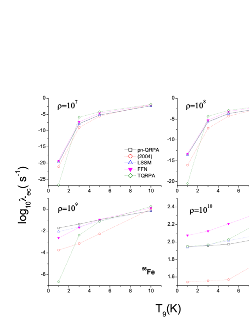
Figure 3: Same as Figure 1 but for ⁵⁶Fe.

The electron capture rate calculations on ⁵⁶Fe is shown in Fig. 3. At density of around 10⁷ gcm^-3 (upper left panel) the comparison of reported rates with LSSM rates is perfect. The previous pn-QRPA calculation and FFN rates differ by up to an order of magnitude with current reported electron capture rates for reasons stated before. The TQRPA rates are suppressed by a whopping seven orders of magnitude at low temperature of T₉ =1. However, by merely changing T₉ =1 to T₉ =1.5, the TQRPA rates increase by as much as up to 4 orders of magnitude bigger than the corresponding pn-QRPA and LSSM rates. It looks that TQRPA rates are very sensitive to temperature changes for the case of ⁵⁶Fe at low densities. The comparison improves with increasing stellar temperatures and densities. Once again at T₉ =10 the TQRPA rates are roughly double the pn-QRPA and LSSM rates. The upper right panel shows the calculated rates at density of 10⁸ gcm^-3. The LSSM rates are in superb agreement whereas FFN rates are bigger by up to an order of magnitude as compared to reported rates. The previous pn-QRPA rates are smaller by up to two orders of magnitude at T₉ =1 and become progressively bigger at higher temperatures. TQRPA comparison is similar as witnessed in upper left panel. The mutual comparison between the five calculations remain more or less same at stellar density of 10⁹ gcm^-3 (lower left panel). It is to be noted that at low temperatures the reported electron capture rates are more than double the LSSM rates. At still higher density of 10¹⁰ gcm^-3 (lower right panel) all calculations agree with one another within a factor of ten as was in the case of ⁵⁴Fe (Fig. 1). Figs. 1 and 3 depict the fact that the comparison between pn-QRPA and LSSM is comparatively far better and that TQRPA model requires further refinement. However during oxygen and silicon burning phases, the reported rates are a factor of 2-4 bigger than LSSM calculated electron capture rates. Core-collapse simulators should take note of these findings which can greatly assist in evolution of fine-tuning of time rate of change of lepton fraction in their codes.

Neutrino cooling rates play a key role in controlling the overall entropy of the stellar matter. As mentioned earlier the calculated neutrino cooling rates contain contributions both due to electron capture and positron decay on iron isotopes. Whereas electron capture rates are orders of magnitude bigger than competing positron decay rates, nonetheless they have a finite contribution to the total neutrino cooling rates and as such are included in the calculation. Figs. 4-6 show four panels depicting neutrino cooling rates due to electron capture and positron decay rates on ^54-56Fe. The upper left, upper right, lower left and lower right panels show neutrino cooling rates calculated at stellar densities of 10⁶, 10⁷, 10⁸ and 10⁹ gcm^-3, respectively. All neutrino cooling rates are shown in logarithmic scale (to base 10) and calculated in units of $MeV.s^{-1}$. Again the density scale in four panels were carefully selected where calculated electron capture and positron decay rates are most effective due to isotopes of iron as per the modeling and simulation results of presupernova evolution of massive stars by Heger and collaborators [4]. Consequently, for the chosen temperature and density zone, the neutrino cooling rates should be most effective in stellar matter.

Fig. 4 show reported neutrino cooling rates due to ⁵⁴Fe in stellar matter. Shown also are the previous pn-QRPA cooling rates (2004) as well as LSSM and FFN results. It is pertinent to mention that TQRPA formalism was not used to calculate the neutrino cooling rates. Rates in upper left panel (plotted at a stellar density of around 10⁶ gcm^-3) show that the previous pn-QRPA rates are, in general, bigger than reported rates by an order of magnitude (except at T₉ =3 where the reported rates are bigger). At T₉ =1 (3) the reported neutrino cooling rates is around four (three) times the LSSM cooling rates. The comparison with LSSM is perfect at higher temperatures. A more or less similar comparison between the different theoretical calculations exist at a stellar density of around 10⁷ gcm^-3 (upper right panel). For still higher density of around 10⁸ gcm^-3 (lower left panel) the reported rates are within an order of magnitude difference with previous pn-QRPA rates. The reported rates are around five times bigger than FFN rates at T₉ =1 and smaller at all higher temperatures (by an order of magnitude). At T₉ =3, the reported rates are twice the LSSM rates. Otherwise the reported rates are in complete agreement with LSSM reported neutrino cooling rates. The reported rates are 1-2 orders of magnitude bigger than previous pn-QRPA rates at low temperatures (T${}_{9}\leq$ 3) and density of 10⁹ gcm^-3 (lower right panel). At high temperatures the previous pn-QRPA rates surpass the reported rates. Similarly the reported rates are a factor 3-7 bigger at low temperatures (T${}_{9}\leq$ 3) compared to FFN rates. At higher temperatures the FFN rates become bigger. LSSM calculated neutrino cooling rates due to ⁵⁴Fe are in perfect agreement with reported rates at a stellar density of 10⁹ gcm^-3. Overall the new pn-QRPA model results are more reliable than previous pn-QRPA calculation (as also reflected in the good comparison of the calculated GT strength distribution with measurements shown earlier) and are attributed to a judicious choice of model parameters stated earlier. FFN cooling rates are generally bigger by an order of magnitude difference. The reason for this artificial enhancement in FFN rates were also discussed earlier. The new pn-QRPA model and LSSM calculations are in very good agreement, both being microscopic in nature.

The calculated neutrino cooling rates due to ⁵⁵Fe using different nuclear models are shown in Fig. 5. The results are shown in a four panel system akin to Fig. 4. The reported neutrino cooling rates is roughly within a factor of ten as compared to previous pn-QRPA and FFN calculations and are found to be in excellent agreement with LSSM calculation. The origin of these differences are already being discussed above.

We finally present the calculations of neutrino cooling rates due to ⁵⁶Fe in Fig. 6. For this case the reported cooling rates are 1-2 orders of magnitude bigger than previous pn-QRPA calculation at low temperatures (T${}_{9}\leq$ 3). The comparison improves at higher temperatures. FFN calculations are within a factor 10 of reported rates while LSSM rates are once again in very good agreement with reported rates for reasons already discussed. During silicon shell burning stages and in later phases the reported neutrino cooling rates is roughly double the LSSM rates. This information may also prove useful for core-collapse simulators. Generally speaking the new pn-QRPA calculated weak rates are in excellent agreement with LSSM rates but at times under some very specific physical conditions (already mentioned) there are some minor differences. Incidentally it is precisely the fine-tuning of the time evolution of lepton-to-baryon fraction (controlled by the stellar weak interaction rates) which may be the key to a successful explosion in the modeling and simulation of core-collapse supernovae.

3 Conclusions

We presented a microscopic calculation of GT strength distribution functions as well as electron capture and neutrino cooling rates due to key iron isotopes in stellar matter. The calculations were also compared with experimental data and other theoretical calculations. These nuclear inputs should prove useful for core-collapse simulators.

The pn-QRPA model places the centroid of the calculated GT strength distributions at much lower energies in daughter nuclei as compared to other RPA interactions. Further the placement of GT centroids by the pn-QRPA model is, in general, in good agreement with the centroids of the measured data. This tendency of pn-QRPA model favor higher values of electron capture rates in stellar environment and can bear significance for astrophysical problems. On the other extreme, the GXPF1 interaction usually leads to placement of GT centroid at much higher energies in daughter compared to other pn-RPA interactions. The reported total GT strengths are, in general, also in good comparison with measured strengths.

During the oxygen and silicon shell and core burning phases of massive stars the pn-QRPA electron capture (neutrino cooling) rates on ⁵⁴Fe are around three times (up to four times) bigger than those calculated by LSSM. The comparison with LSSM gets better for proceeding pre-supernova and supernova phases of stars. The pn-QRPA calculated electron capture rates on ^55,56Fe are in overall excellent agreement with the LSSM rates. During silicon shell burning for stars ($\sim 10-25M_{\odot}$) and oxygen shell burning for much heavier stars ($\sim 40M_{\odot}$) the calculated cooling rates due to ⁵⁵Fe are in very good comparison with the LSSM rates. The results for neutrino cooling rates due to ⁵⁶Fe are in overall good agreement with the corresponding LSSM numbers. FFN rates, in general, are 1-2 orders of magnitude bigger.

The weak rates were calculated on a fine-grid scale, of great utility for core-collapse simulators, and also suitable for interpolation purposes. We present a sample of our fine-grid scale calculation of weak rates at a stellar density of 10¹¹ gcm^-3 in Table 5. The ASCII file of the complete table can be requested from the corresponding author. It is expected that the present calculation can contribute to a better understanding of the explosion mechanism of massive stars. However significant progress is expected, in part, to come from next-generation radioactive ion-beam facilities (e.g. FAIR (Germany), FRIB (USA) and FRIB (Japan)) when we would have access to measured GT strength distribution of many more nuclei (including unstable isotopes).

References

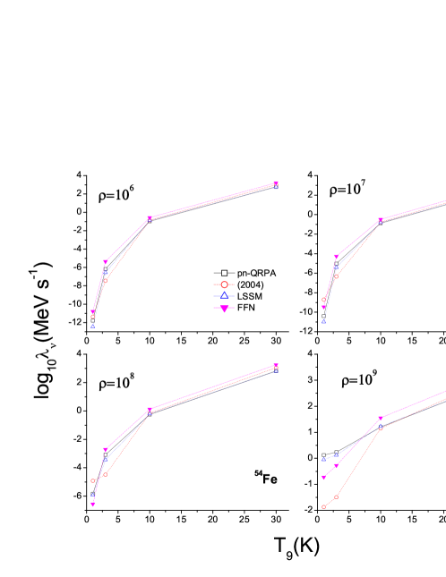
Figure 4: Comparison of neutrino cooling rates due to ⁵⁴Fe using current pn-QRPA model (pn-QRPA), previous pn-QRPA calculation (2004) [13], shell model calculation (LSSM) [25] and calculation done by Ref. [26] (FFN) at different selected stellar temperature and density zones.

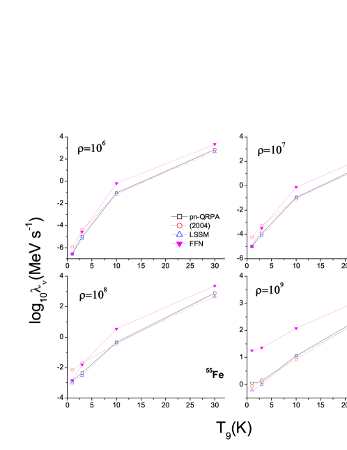
Figure 5: Same as Figure 4 but for ⁵⁵Fe.

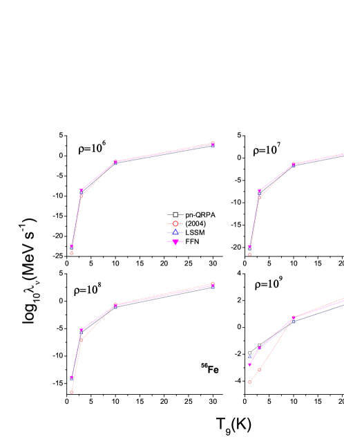
Figure 6: Same as Figure 4 but for ⁵⁶Fe.

Table 1: Calculated GT strength distributions in the electron capture direction for ⁵⁴Fe using different pn-RPA scenarios. For details of interactions used see text. Calculated GT strength less than $10^{-3}$ is not given to save space. Measured data (Exp) is taken from Ref. [18].

KB3G		GXPF1		FPD6		pn-QRPA		Exp
$E_{i}$	$B(GT_{+})$	$E_{i}$	$B(GT_{+})$	$E_{i}$	$B(GT_{+})$	$E_{i}$	$B(GT_{+})$	$E_{i}$	$B(GT_{+})$
4.93	1.50 $\times 10^{-2}$	4.68	3.39 $\times 10^{-3}$	5.19	1.49 $\times 10^{-2}$	1.39	3.56 $\times 10^{-1}$	-1.5	0.05
4.93	1.18 $\times 10^{-2}$	4.68	3.39 $\times 10^{-3}$	5.19	1.49 $\times 10^{-2}$	1.45	6.33 $\times 10^{-2}$	-0.5	0.12
4.93	1.18 $\times 10^{-2}$	4.83	8.78 $\times 10^{-3}$	5.29	2.46 $\times 10^{-2}$	1.61	5.37 $\times 10^{-2}$	0.5	0.25
5.41	4.32 $\times 10^{-3}$	5.05	7.52 $\times 10^{-3}$	5.54	5.37 $\times 10^{-2}$	1.78	3.01 $\times 10^{-2}$	1.5	0.45
5.41	4.32 $\times 10^{-3}$	5.05	7.52 $\times 10^{-3}$	5.54	5.37 $\times 10^{-2}$	1.86	2.60 $\times 10^{-2}$	2.5	0.57
5.60	7.30 $\times 10^{-2}$	5.67	1.80 $\times 10^{-2}$	5.73	3.04 $\times 10^{-2}$	2.24	1.90 $\times 10^{-2}$	3.5	0.54
5.60	7.30 $\times 10^{-2}$	5.67	1.80 $\times 10^{-2}$	5.73	3.04 $\times 10^{-2}$	2.36	1.08 $\times 10^{-1}$	4.5	0.51
5.84	8.09 $\times 10^{-2}$	5.76	3.85 $\times 10^{-3}$	6.00	7.94 $\times 10^{-2}$	2.59	2.89 $\times 10^{-3}$	5.5	0.38
5.84	8.09 $\times 10^{-2}$	5.82	2.28 $\times 10^{-2}$	6.00	7.94 $\times 10^{-2}$	2.70	2.83 $\times 10^{-2}$	6.5	0.41
6.16	1.49 $\times 10^{-1}$	5.82	2.28 $\times 10^{-2}$	6.44	2.80 $\times 10^{-2}$	2.72	1.77 $\times 10^{-1}$	7.5	0.19
6.18	8.04 $\times 10^{-2}$	6.05	2.22 $\times 10^{-2}$	6.44	2.80 $\times 10^{-2}$	2.97	5.43 $\times 10^{-2}$	8.5	0.05
6.18	8.04 $\times 10^{-2}$	6.05	2.22 $\times 10^{-2}$	6.51	1.50 $\times 10^{-1}$	3.05	4.39 $\times 10^{-2}$
6.50	1.35 $\times 10^{-1}$	6.29	5.50 $\times 10^{-2}$	6.96	3.98 $\times 10^{-1}$	3.09	4.28 $\times 10^{-3}$
6.50	1.35 $\times 10^{-1}$	7.11	3.99 $\times 10^{-2}$	6.96	3.98 $\times 10^{-1}$	3.40	2.70 $\times 10^{-2}$
6.78	7.14 $\times 10^{-1}$	7.11	3.99 $\times 10^{-2}$	7.24	6.19 $\times 10^{-1}$	3.49	3.07 $\times 10^{-2}$
6.78	7.14 $\times 10^{-1}$	7.70	5.12 $\times 10^{-1}$	7.24	6.19 $\times 10^{-1}$	3.57	1.93 $\times 10^{-1}$
6.84	5.17 $\times 10^{-1}$	7.70	5.12 $\times 10^{-1}$	7.24	3.23 $\times 10^{-1}$	3.83	2.62 $\times 10^{-1}$
7.32	2.73 $\times 10^{-2}$	7.72	4.25 $\times 10^{-1}$	8.13	3.73 $\times 10^{-2}$	3.89	3.53 $\times 10^{-2}$
7.46	1.89 $\times 10^{-1}$	8.07	7.28 $\times 10^{-2}$	8.13	3.73 $\times 10^{-2}$	3.90	1.16 $\times 10^{-3}$
7.46	1.89 $\times 10^{-1}$	8.13	1.51 $\times 10^{-1}$	8.15	2.31 $\times 10^{-1}$	4.08	1.19 $\times 10^{-3}$
7.67	3.86 $\times 10^{-2}$	8.13	1.51 $\times 10^{-1}$	8.44	3.08 $\times 10^{-2}$	4.15	4.05 $\times 10^{-2}$
7.67	3.86 $\times 10^{-2}$	8.16	6.46 $\times 10^{-1}$	8.44	3.08 $\times 10^{-2}$	4.34	2.18 $\times 10^{-2}$
8.16	9.56 $\times 10^{-2}$	8.16	6.46 $\times 10^{-1}$	8.80	3.31 $\times 10^{-2}$	4.38	2.22 $\times 10^{-3}$
8.16	9.56 $\times 10^{-2}$	9.13	1.68 $\times 10^{-1}$	8.80	3.31 $\times 10^{-2}$	4.60	1.67 $\times 10^{-2}$
8.30	1.07 $\times 10^{0}$	9.13	1.68 $\times 10^{-1}$	9.11	8.56 $\times 10^{-1}$	4.68	1.27 $\times 10^{-1}$
		9.73	1.44 $\times 10^{0}$			4.92	7.14 $\times 10^{-3}$
						4.97	3.01 $\times 10^{-2}$
						5.03	1.84 $\times 10^{-3}$
						5.25	5.38 $\times 10^{-2}$
						5.38	1.50 $\times 10^{-1}$
						5.61	5.68 $\times 10^{-3}$
						5.64	1.11 $\times 10^{-3}$
						5.71	3.44 $\times 10^{-2}$
						5.77	2.26 $\times 10^{-2}$
						5.83	8.02 $\times 10^{-3}$
						5.92	5.56 $\times 10^{-2}$
						6.12	4.14 $\times 10^{-3}$
						6.14	2.66 $\times 10^{-2}$
						6.15	1.05 $\times 10^{-2}$
						6.24	1.09 $\times 10^{-2}$
						6.44	1.22 $\times 10^{-3}$
						6.47	2.65 $\times 10^{-2}$
						6.50	5.61 $\times 10^{-2}$
						6.86	1.15 $\times 10^{-2}$
						6.97	3.52 $\times 10^{-3}$
						7.13	4.45 $\times 10^{-1}$
						7.56	1.25 $\times 10^{-3}$
						7.80	1.23 $\times 10^{-3}$
						7.85	1.74 $\times 10^{-3}$
						10.17	4.76$\times 10^{-3}$
						10.31	2.96$\times 10^{-2}$
						10.49	9.95$\times 10^{-2}$
						10.57	2.02$\times 10^{-3}$
						10.88	4.90$\times 10^{-1}$
						10.98	5.92$\times 10^{-3}$
						11.06	2.91$\times 10^{-2}$
						11.12	1.89$\times 10^{-1}$
						11.26	3.90$\times 10^{-2}$

Table 2: Same as Table 1 but for ⁵⁵Fe.

KB3G		GXPF1		FPD6		pn-QRPA
$E_{i}$	$B(GT_{+})$	$E_{i}$	$B(GT_{+})$	$E_{i}$	$B(GT_{+})$	$E_{i}$	$B(GT_{+})$
0.65	2.75 $\times 10^{-3}$	0.21	5.28 $\times 10^{-3}$	0.52	7.30 $\times 10^{-3}$	0.00	2.55 $\times 10^{-3}$
0.66	3.75 $\times 10^{-3}$	0.23	8.35 $\times 10^{-3}$	0.58	1.14 $\times 10^{-2}$	1.29	2.88 $\times 10^{-2}$
1.27	4.70 $\times 10^{-3}$	0.67	1.01 $\times 10^{-2}$	1.03	5.80 $\times 10^{-3}$	2.17	1.13 $\times 10^{-1}$
1.30	1.05 $\times 10^{-2}$	1.00	3.30 $\times 10^{-2}$	1.05	1.49 $\times 10^{-2}$	2.57	2.76 $\times 10^{-2}$
1.58	4.45 $\times 10^{-2}$	1.41	4.42 $\times 10^{-3}$	1.30	8.94 $\times 10^{-3}$	2.66	1.91 $\times 10^{-3}$
1.70	1.51 $\times 10^{-2}$	1.41	4.20 $\times 10^{-3}$	1.79	3.52 $\times 10^{-2}$	2.94	3.71 $\times 10^{-2}$
1.70	1.59 $\times 10^{-2}$	1.60	1.32 $\times 10^{-2}$	1.82	3.20 $\times 10^{-2}$	3.88	4.40 $\times 10^{-3}$
2.07	1.86 $\times 10^{-2}$	1.60	1.36 $\times 10^{-2}$	1.93	5.47 $\times 10^{-2}$	4.70	2.08 $\times 10^{-3}$
2.07	2.51 $\times 10^{-2}$	2.10	6.48 $\times 10^{-3}$	2.24	8.67 $\times 10^{-2}$	4.98	4.27 $\times 10^{-2}$
2.19	9.45 $\times 10^{-3}$	2.10	1.56 $\times 10^{-2}$	2.25	9.90 $\times 10^{-2}$	5.05	7.64 $\times 10^{-2}$
2.22	9.18 $\times 10^{-2}$	2.20	2.27 $\times 10^{-2}$	2.41	2.12 $\times 10^{-3}$	5.06	3.81 $\times 10^{-3}$
2.29	1.67 $\times 10^{-1}$	2.35	5.43 $\times 10^{-3}$	2.43	1.40 $\times 10^{-2}$	5.22	1.47 $\times 10^{-1}$
2.32	1.98 $\times 10^{-2}$	2.37	5.47 $\times 10^{-3}$	2.69	4.54 $\times 10^{-2}$	5.28	1.83 $\times 10^{-2}$
2.52	8.75 $\times 10^{-3}$	2.39	2.56 $\times 10^{-3}$	2.70	1.09 $\times 10^{-1}$	5.32	1.81 $\times 10^{-3}$
2.62	3.19 $\times 10^{-2}$	2.45	3.42 $\times 10^{-2}$	2.89	3.32 $\times 10^{-2}$	5.41	8.02 $\times 10^{-3}$
2.79	1.62 $\times 10^{-3}$	2.53	3.85 $\times 10^{-2}$	2.92	7.46 $\times 10^{-3}$	5.57	6.72 $\times 10^{-2}$
2.79	9.10 $\times 10^{-3}$	2.72	1.17 $\times 10^{-3}$	3.06	1.38 $\times 10^{-3}$	6.68	1.39 $\times 10^{-1}$
2.80	2.76 $\times 10^{-3}$	2.86	6.17 $\times 10^{-3}$	3.09	5.68 $\times 10^{-3}$	6.76	3.80 $\times 10^{-2}$
2.85	2.01 $\times 10^{-2}$	2.88	4.12 $\times 10^{-3}$	3.16	3.72 $\times 10^{-2}$	6.87	1.90 $\times 10^{-1}$
2.92	4.36 $\times 10^{-2}$	2.89	5.24 $\times 10^{-3}$	3.21	2.33 $\times 10^{-3}$	6.89	5.94 $\times 10^{-2}$
2.99	3.16 $\times 10^{-2}$	3.04	2.24 $\times 10^{-2}$	3.36	1.01 $\times 10^{-3}$	7.04	2.83 $\times 10^{-2}$
3.02	1.97 $\times 10^{-2}$	3.12	4.62 $\times 10^{-3}$	3.43	2.26 $\times 10^{-1}$	7.30	3.19 $\times 10^{-1}$
3.17	1.40 $\times 10^{-2}$	3.12	4.75 $\times 10^{-3}$	3.53	5.98 $\times 10^{-2}$	7.35	8.70 $\times 10^{-3}$
3.23	5.88 $\times 10^{-2}$	3.30	6.75 $\times 10^{-2}$	3.80	3.52 $\times 10^{-2}$	7.54	4.33 $\times 10^{-2}$
3.33	6.74 $\times 10^{-2}$	3.42	2.14 $\times 10^{-2}$	3.98	1.51 $\times 10^{-1}$	7.62	1.13 $\times 10^{-2}$
3.39	1.40 $\times 10^{-1}$	3.45	2.43 $\times 10^{-2}$	4.11	3.50 $\times 10^{-1}$	7.66	1.60 $\times 10^{-2}$
3.50	1.75 $\times 10^{-1}$	3.76	8.23 $\times 10^{-2}$	4.29	1.40 $\times 10^{-1}$	7.72	9.35 $\times 10^{-2}$
3.66	4.00 $\times 10^{-1}$	3.79	7.81 $\times 10^{-2}$	4.36	8.62 $\times 10^{-2}$	7.75	6.00 $\times 10^{-2}$
3.73	2.32 $\times 10^{-1}$	3.96	3.30 $\times 10^{-2}$	4.39	1.48 $\times 10^{-1}$	8.00	5.78 $\times 10^{-1}$
3.77	6.56 $\times 10^{-2}$	4.03	4.13 $\times 10^{-2}$	4.45	1.85 $\times 10^{-2}$	8.02	3.44 $\times 10^{-2}$
3.77	1.59 $\times 10^{-1}$	4.09	1.10 $\times 10^{-2}$	4.46	2.31 $\times 10^{-2}$	8.07	4.51 $\times 10^{-3}$
3.81	1.12 $\times 10^{-1}$	4.15	2.97 $\times 10^{-1}$	4.61	1.25 $\times 10^{-1}$	8.10	6.44 $\times 10^{-2}$
3.92	1.34 $\times 10^{-1}$	4.19	7.81 $\times 10^{-2}$	4.70	8.06 $\times 10^{-2}$	8.21	5.66 $\times 10^{-3}$
3.95	1.54 $\times 10^{-1}$	4.28	8.11 $\times 10^{-2}$	4.78	6.59 $\times 10^{-2}$	8.27	1.65 $\times 10^{-2}$
4.00	3.74 $\times 10^{-3}$	4.30	1.52 $\times 10^{-2}$	4.81	1.51 $\times 10^{-2}$	8.28	1.43 $\times 10^{-2}$
4.17	3.87 $\times 10^{-2}$	4.31	3.61 $\times 10^{-2}$	4.93	1.63 $\times 10^{-2}$	8.30	4.52 $\times 10^{-3}$
4.19	6.99 $\times 10^{-2}$	4.43	2.24 $\times 10^{-1}$	5.13	2.87 $\times 10^{-2}$	8.36	2.52 $\times 10^{-1}$
4.23	1.16 $\times 10^{-3}$	4.47	1.32 $\times 10^{-1}$	5.13	8.34 $\times 10^{-2}$	8.36	4.62 $\times 10^{-2}$
4.23	1.99 $\times 10^{-2}$	4.72	3.63 $\times 10^{-1}$	5.19	6.48 $\times 10^{-2}$	8.43	1.14 $\times 10^{-1}$
4.40	8.37 $\times 10^{-2}$	4.81	6.58 $\times 10^{-2}$	5.20	3.24 $\times 10^{-2}$	8.65	1.68 $\times 10^{-3}$
4.41	6.65 $\times 10^{-2}$	4.85	5.28 $\times 10^{-3}$	5.59	2.53 $\times 10^{-3}$	8.85	6.87 $\times 10^{-3}$
4.59	1.95 $\times 10^{-2}$	4.92	3.33 $\times 10^{-1}$	5.60	5.20 $\times 10^{-2}$	8.93	6.01 $\times 10^{-2}$
4.59	1.36 $\times 10^{-2}$	4.94	5.36 $\times 10^{-2}$	5.66	3.06 $\times 10^{-3}$	8.95	1.28 $\times 10^{-1}$
4.89	1.42 $\times 10^{-2}$	5.04	2.19 $\times 10^{-1}$	5.90	2.90 $\times 10^{-1}$	9.17	2.60 $\times 10^{-3}$
4.89	2.37 $\times 10^{-1}$	5.21	3.10 $\times 10^{-1}$	6.01	3.06 $\times 10^{-3}$	9.25	3.18 $\times 10^{-3}$
4.98	2.48 $\times 10^{-2}$	5.24	1.83 $\times 10^{-1}$	6.35	2.82 $\times 10^{-1}$	9.30	4.77 $\times 10^{-3}$
5.09	2.67 $\times 10^{-2}$	5.46	5.88 $\times 10^{-2}$	6.39	3.54 $\times 10^{-2}$	9.51	1.43 $\times 10^{-2}$
5.12	2.66 $\times 10^{-1}$	5.59	9.05 $\times 10^{-3}$	6.47	3.22 $\times 10^{-2}$	9.66	1.85 $\times 10^{-3}$
5.21	5.22 $\times 10^{-2}$	5.63	8.05 $\times 10^{-2}$	6.56	1.67 $\times 10^{-2}$	9.69	1.08 $\times 10^{-3}$
5.53	9.35 $\times 10^{-3}$	5.95	1.32 $\times 10^{-2}$	6.78	7.69 $\times 10^{-3}$	9.69	5.38 $\times 10^{-3}$
5.54	5.59 $\times 10^{-2}$	6.09	2.54 $\times 10^{-3}$	7.03	1.19 $\times 10^{-2}$	10.05	6.35 $\times 10^{-3}$
5.60	3.20 $\times 10^{-1}$	6.19	1.35 $\times 10^{-1}$	7.06	7.30 $\times 10^{-2}$	10.06	2.60 $\times 10^{-3}$
5.63	2.76 $\times 10^{-2}$	6.24	3.05 $\times 10^{-2}$	7.27	1.71 $\times 10^{-3}$	10.09	7.04 $\times 10^{-3}$
5.70	1.84 $\times 10^{-2}$	6.40	1.89 $\times 10^{-1}$	7.30	3.45 $\times 10^{-3}$	10.16	1.81 $\times 10^{-3}$
5.74	2.73 $\times 10^{-2}$	6.46	2.78 $\times 10^{-2}$	7.64	2.48 $\times 10^{-2}$	13.97	1.37 $\times 10^{-3}$
5.96	7.45 $\times 10^{-2}$	6.65	7.02 $\times 10^{-1}$	7.90	2.08 $\times 10^{-3}$
6.06	2.99 $\times 10^{-3}$	6.81	1.27 $\times 10^{-2}$
6.16	3.06 $\times 10^{-2}$	6.84	2.22 $\times 10^{-1}$
6.23	2.21 $\times 10^{-3}$	7.19	2.46 $\times 10^{-3}$
6.49	1.88 $\times 10^{-3}$	7.19	1.05 $\times 10^{-2}$

Table 3: Same as Table 1 but for ⁵⁶Fe. Measured data (Exp) is taken from Ref. [20].

KB3G		GXPF1		FPD6		pn-QRPA		Exp
$E_{i}$	$B(GT_{+})$	$E_{i}$	$B(GT_{+})$	$E_{i}$	$B(GT_{+})$	$E_{i}$	$B(GT_{+})$	$E_{i}$	$B(GT_{+})$
3.46	3.12 $\times 10^{-1}$	3.83	1.46 $\times 10^{-1}$	3.90	3.69 $\times 10^{-1}$	0.11	3.82 $\times 10^{-2}$	-2.0	0.0084
3.46	3.12 $\times 10^{-1}$	3.83	1.46 $\times 10^{-1}$	3.90	3.69 $\times 10^{-1}$	0.22	2.53 $\times 10^{-1}$	-1.0	0.13
4.80	2.75 $\times 10^{-2}$	4.94	2.13 $\times 10^{-2}$	5.27	8.48 $\times 10^{-3}$	0.77	2.42 $\times 10^{-3}$	0.0	0.40
4.86	2.54 $\times 10^{-1}$	5.36	6.89 $\times 10^{-2}$	5.27	8.48 $\times 10^{-3}$	0.83	1.14 $\times 10^{-2}$	1.0	0.57
4.86	2.54 $\times 10^{-1}$	5.36	6.89 $\times 10^{-2}$	5.83	9.83 $\times 10^{-2}$	1.18	9.14 $\times 10^{-3}$	2.0	0.56
5.42	1.92 $\times 10^{-1}$	5.51	8.41 $\times 10^{-2}$	5.97	2.28 $\times 10^{-1}$	1.24	1.00 $\times 10^{-2}$	3.0	0.29
5.42	2.40 $\times 10^{-1}$	5.95	1.57 $\times 10^{-1}$	5.97	2.28 $\times 10^{-1}$	1.29	4.44 $\times 10^{-2}$	4.0	0.27
5.42	2.40 $\times 10^{-1}$	5.95	1.56 $\times 10^{-1}$	6.72	6.62 $\times 10^{-2}$	1.56	1.55 $\times 10^{-1}$	5.0	0.15
5.88	9.99 $\times 10^{-2}$	6.02	4.88 $\times 10^{-1}$	6.76	1.32 $\times 10^{-1}$	1.73	5.53 $\times 10^{-3}$	6.0	0.14
5.88	9.99 $\times 10^{-2}$	6.02	4.88 $\times 10^{-1}$	6.76	1.32 $\times 10^{-1}$	1.98	4.79 $\times 10^{-2}$	7.0	0.14
5.96	3.22 $\times 10^{-2}$	6.64	3.04 $\times 10^{-1}$	7.04	3.32 $\times 10^{-2}$	2.31	2.52 $\times 10^{-2}$	8.0	0.19
6.56	7.62 $\times 10^{-3}$	6.73	1.86 $\times 10^{-2}$	7.04	3.32 $\times 10^{-2}$	2.48	2.62 $\times 10^{-3}$	9.0	0.17
6.56	7.62 $\times 10^{-3}$	6.73	1.86 $\times 10^{-2}$	7.19	2.89 $\times 10^{-2}$	2.55	5.90 $\times 10^{-2}$	10.0	0.22
6.66	6.95 $\times 10^{-1}$	7.40	2.56 $\times 10^{-1}$	8.10	5.14 $\times 10^{-1}$	2.62	4.39 $\times 10^{-2}$
7.21	6.04 $\times 10^{-2}$	7.40	2.56 $\times 10^{-1}$	8.77	2.47 $\times 10^{-2}$	2.67	7.38 $\times 10^{-2}$
7.21	6.04 $\times 10^{-2}$	7.75	1.28 $\times 10^{-2}$	8.77	2.47 $\times 10^{-2}$	2.77	3.70 $\times 10^{-2}$
7.71	1.02 $\times 10^{-2}$	7.97	7.79 $\times 10^{-3}$	9.18	1.58 $\times 10^{-2}$	2.77	6.00 $\times 10^{-2}$
7.71	1.02 $\times 10^{-2}$	7.97	7.79 $\times 10^{-3}$	9.18	1.58 $\times 10^{-2}$	2.79	7.36 $\times 10^{-2}$
7.90	1.51 $\times 10^{-1}$	8.48	9.14 $\times 10^{-1}$	9.89	5.12 $\times 10^{-2}$	2.89	3.16 $\times 10^{-3}$
8.09	1.90 $\times 10^{-2}$	8.84	4.14 $\times 10^{-2}$	10.10	1.69 $\times 10^{-3}$	3.00	2.11 $\times 10^{-2}$
8.09	1.90 $\times 10^{-2}$	8.84	4.14 $\times 10^{-2}$	10.10	1.69 $\times 10^{-3}$	3.07	1.07 $\times 10^{-2}$
						3.22	8.47 $\times 10^{-3}$
						3.26	3.39 $\times 10^{-2}$
						3.33	1.34 $\times 10^{-3}$
						3.75	9.74 $\times 10^{-2}$
						3.78	2.55 $\times 10^{-3}$
						3.86	1.59 $\times 10^{-3}$
						4.02	8.90 $\times 10^{-1}$
						4.33	5.49 $\times 10^{-2}$
						4.54	7.37 $\times 10^{-2}$
						4.66	2.17 $\times 10^{-2}$
						4.70	2.62 $\times 10^{-2}$
						4.75	1.63 $\times 10^{-2}$
						4.83	1.15 $\times 10^{-3}$
						5.03	2.14 $\times 10^{-2}$
						5.08	4.90 $\times 10^{-3}$
						5.13	8.44 $\times 10^{-3}$
						5.15	2.68 $\times 10^{-3}$
						5.23	2.47 $\times 10^{-3}$
						5.31	1.54 $\times 10^{-2}$
						5.43	1.58 $\times 10^{-3}$
						5.47	1.84 $\times 10^{-2}$
						5.53	1.80 $\times 10^{-3}$
						6.07	5.96 $\times 10^{-3}$
						6.07	1.06 $\times 10^{-2}$
						6.10	2.23 $\times 10^{-2}$
						6.15	5.12 $\times 10^{-3}$
						6.28	1.43 $\times 10^{-3}$
						6.49	2.95 $\times 10^{-3}$
						6.55	4.98 $\times 10^{-3}$
						6.83	1.01 $\times 10^{-3}$
						7.06	3.05 $\times 10^{-3}$

Table 4: Statistics of calculated GT strength distributions for nuclei using different RPA models given in second column. For references of theoretical calculations see text, while experimental references are: (a) $\rightarrow$ [18], (b) $\rightarrow$ [21], (c) $\rightarrow$ [22], (d) $\rightarrow$ [23], (e) $\rightarrow$ [24], (f) $\rightarrow$ [20].

Nucleus	Model	E(GT+)	Width(GT+)	$\sum B(GT_{+})$	E(GT-)	Width(GT-)	$\sum B(GT_{-})$
		MeV	MeV	arb. units	MeV	MeV	arb. units
54Fe
	FPD6	7.50	1.01	4.23	11.92	2.56	7.83
	GXPF1	8.42	1.00	5.19	12.97	2.59	8.79
	KB3G	7.13	0.83	4.62	11.02	2.34	8.24
	pn-QRPA	5.80	3.38	3.59	8.03	4.40	7.41
	EXP(a)	3.7	2.2	3.5	-	-	-
	EXP(b)	3.0	2.3	3.1	8.3	3.6	7.5
	EXP(c)	-	-	-	7.4	3.1	4.0
	EXP(d)	-	-	-	-	-	7.8
	EXP(e)	-	-	-	7.6	3.2	6.0
55Fe
	FPD6	4.42	1.43	3.21	14.87	3.02	8.61
	GXPF1	5.07	1.26	4.52	15.93	3.24	9.92
	KB3G	4.03	1.08	3.82	13.96	2.95	9.22
	pn-QRPA	7.12	1.75	2.98	13.68	5.77	8.31
56Fe
	FPD6	6.12	1.75	2.38	12.79	3.00	9.58
	GXPF1	6.73	1.38	3.70	14.09	3.39	10.90
	KB3G	5.49	1.32	3.10	12.54	3.13	10.30
	pn-QRPA	3.14	1.53	2.36	7.79	3.79	9.99
	EXP(a)	2.7	2.0	2.3	-	-	-
	EXP(d)	-	-	-	-	-	9.9
	EXP(f)	3.5	3.2	3.2	-	-	-

Table 5: Fine-grid calculation of electron capture and neutrino cooling rates due to ^54,55,56Fe for selected stellar density of 10${}^{11}g/cm^{3}$ as a function of temperature in stellar matter. log$\rho Y_{e}$ has units of $g/cm^{3}$, where $\rho$ is the baryon density and $Y_{e}$ is the ratio of the lepton number to the baryon number. Temperatures ($T_{9}$) are given in units of $10^{9}$ K. The calculated Fermi energy is denoted by $E_{f}$ and is given in units of MeV. $\lambda_{ec}$ ($\lambda_{\nu}$) are the electron capture (neutrino cooling) rates in units of $s^{-1}$ ($MeVs^{-1}$). All calculated rates are tabulated in logarithmic (to base 10) scale.

$log\rho Y_{e}$	$T_{9}$	$E_{f}$	54Fe		55Fe		56Fe
			$\lambda_{ec}$	$\lambda_{\nu}$	$\lambda_{ec}$	$\lambda_{\nu}$	$\lambda_{ec}$	$\lambda_{\nu}$
11.0	0.50	23.934	4.408	5.593	4.355	5.493	4.255	5.389
11.0	1.00	23.933	4.408	5.593	4.355	5.493	4.255	5.389
11.0	1.50	23.932	4.409	5.594	4.355	5.492	4.255	5.390
11.0	2.00	23.930	4.409	5.594	4.355	5.492	4.255	5.390
11.0	2.50	23.928	4.409	5.594	4.355	5.493	4.256	5.390
11.0	3.00	23.925	4.409	5.595	4.356	5.494	4.256	5.390
11.0	3.50	23.922	4.410	5.596	4.357	5.496	4.256	5.390
11.0	4.00	23.918	4.411	5.596	4.358	5.499	4.257	5.390
11.0	4.50	23.913	4.411	5.597	4.360	5.502	4.257	5.390
11.0	5.00	23.908	4.412	5.598	4.362	5.505	4.258	5.390
11.0	5.50	23.903	4.413	5.600	4.364	5.508	4.259	5.391
11.0	6.00	23.897	4.414	5.601	4.367	5.512	4.260	5.392
11.0	6.50	23.891	4.416	5.603	4.369	5.516	4.261	5.393
11.0	7.00	23.884	4.417	5.605	4.372	5.521	4.262	5.395
11.0	7.50	23.877	4.419	5.607	4.376	5.526	4.264	5.397
11.0	8.00	23.869	4.421	5.610	4.380	5.532	4.266	5.399
11.0	8.50	23.860	4.423	5.613	4.384	5.538	4.269	5.402
11.0	9.00	23.851	4.426	5.617	4.389	5.545	4.272	5.406
11.0	9.50	23.842	4.429	5.621	4.395	5.552	4.275	5.410
11.0	10.00	23.832	4.432	5.626	4.401	5.560	4.278	5.415
11.0	15.00	23.704	4.481	5.696	4.481	5.666	4.335	5.492
11.0	20.00	23.526	4.543	5.784	4.568	5.787	4.406	5.594
11.0	25.00	23.296	4.599	5.865	4.645	5.900	4.471	5.689
11.0	30.00	23.016	4.648	5.937	4.712	6.000	4.527	5.773

References

- [1] Bethe H A, 1939 Phys. Rev. 55 434.
- [2] Bethe H A, 1990 Rev. Mod. Phys. 62 801.
- [3] Strother T and Bauer W, 2009 Prog. Part. Nucl. Phys. 62 468.
- [4] Heger A, Woosley S E, Martínez-Pinedo G and Langanke K, 2001 Astrophys. J. 560 307.
- [5] Aufderheide M B, Fushiki I, Woosley S E, Stanford E and Hartmann D H, 1994 Astrophys. J. Suppl. Ser 91 389.
- [6] Nabi J-Un, 2009 Eur. Phys. J. 40 223.
- [7] Nabi J-Un, 2011 Astrophys. Space Sci. 331 537.
- [8] Nabi J-Un, 2011 Adv. Space Research 48 985.
- [9] Nabi J-Un, 2012 Rom. J. Phys. 57 1211.
- [10] Nabi J-Un and Tawfik A N, 2013 Phys. Atom. Nucl. 76 294.
- [11] Halbleib J A and Sorensen R A, 1967 Nucl. Phys. A98 542.
- [12] Muto K, Bender E, Oda T and Klapdor H V, 1992 Zeit. Phys. A341 407.
- [13] Nabi J-Un and Klapdor-Kleingrothaus H V 2004 At. Data Nucl. Data Tables 88 237.
- [14] Nabi J-Un and Johnson C W, 2013 J. Phys. G 40 065202.
- [15] Poves A, Sánchez-Solano J, Caurier E and Nowacki F, 2001 Nucl. Phys A 694 157.
- [16] Honma M, Otsuka T, Brown B A and Mizusaki T, 2004 Phys. Rev. C 65 061301(R); 69, 034335.
- [17] Richter W A, Van der Merwe M G, Julies R E and Brown B A, 1991 Nucl. Phys A 523 325.
- [18] Rönnqvist T, Condé H, Olsson N, Ramström E, Zorro R, Blomgren J, Håkansson A, Ringbom A, Tibell G, Jonsson O, Nilsson L, Renberg P-U, van der Werf S Y, Unkelbach W and Brady F P, 1993 Nucl. Phys. A 563 225.
- [19] Nabi J-Un, 2010 Adv. Space Research 46 1191.
- [20] El-Kateb S, Jackson K P, Alford W P, Abegg R, Azuma R E, Brown B A, Celler A, Frekers D, Häusser O, Helmer R, Henderson R S, Hicks K H, Jeppesen R, King J D, Raywood K, Shute G G, Spicer B M, Trudel A, Vetterli M and Yen S, 1994 Phys. Rev. C 49 3128.
- [21] Vetterli M C, Häusser O, Abegg R, Alford W P, Celler A, Frekers D, Helmer R, Henderson R, Hicks K H, Jackson K P, Jeppesen R G, Miller C A, Raywood K and Yen S, 1989 Phys. Rev. C 40 559.
- [22] Adachi T et. al, 2012 Phys. Rev. C 85 024308.
- [23] Rapaport J, Taddeucci T, Welch T P, Gaarde C, Larsen J, Horen D J, Sugarbaker E, Koncz P, Foster C C, Goodman C D, Goulding C A and Masterson T, 1983 Nucl. Phys. A 410 371.
- [24] Anderson B D, Lebo C, Baldwin A R, Chittrakarn T, Madey R and Watson J W, 1990 Phys. Rev. C 41 1474.
- [25] Langanke K and Martínez-Pinedo G, 2000 Nucl. Phys.A673 481.
- [26] Fuller G M, Fowler W A and Newman M J, 1980 Astrophys. J. Suppl. 42 447; 1982 Astrophys. J. Suppl. 48 279; 1982 Astrophys. J. 252 715; 1985 Astrophys. J. 293 1.
- [27] Dzhioev A A, Vdovin A I, Ponomarev V Yu, Wambach J, Langanke K and Martínez-Pinedo G, 2010 Phys. Rev. C 81, 015804.
- [28] Stetcu I and Johnson C W, 2004 Phys. Rev. C 69, 024311-1 - 024311-7.
- [29] Raman S, Malarkey C H, Milner W T, Nestor, Jr C W and Stelson P H, 1987 At. Data Nucl. Data Tables 36, 1-96.