Discretization of functionals involving the Monge-Ampère operator

Abstract.

Gradient flows in the Wasserstein space have become a powerful tool in the analysis of diffusion equations, following the seminal work of Jordan, Kinderlehrer and Otto (JKO). The numerical applications of this formulation have been limited by the difficulty to compute the Wasserstein distance in dimension $\geqslant 2$. One step of the JKO scheme is equivalent to a variational problem on the space of convex functions, which involves the Monge-Ampère operator. Convexity constraints are notably difficult to handle numerically, but in our setting the internal energy plays the role of a barrier for these constraints. This enables us to introduce a consistent discretization, which inherits convexity properties of the continuous variational problem. We show the effectiveness of our approach on nonlinear diffusion and crowd-motion models.

1. Introduction

1.1. Context

Optimal transport and displacement convexity

In the following, we consider two probability measures $\mu$ and $\nu$ on $\mathbb{R}^{d}$ with finite second moments, the first of which is absolutely continuous with respect to the Lebesgue measure. We are interested in the quadratic optimal transport problem between $\mu$ and $\nu$:

$$\min\left\{\int_{X}\left\|T(x)-x\right\|^{2}\operatorname{d}\mu(x);\,T:X\to\mathbb{R}^{d},~{}T_{\#}\mu=\nu\right\}$$ (1.1)

where $T_{\#}\mu$ denotes the pushforward of $\mu$ by $T$. A theorem of Brenier shows that the optimal map in (1.1) is given by the gradient of a convex function [8]. Define the Wasserstein distance between $\mu$ and $\nu$ as the square root of the minimum in (1.1), and denote it $\operatorname{W}_{2}(\mu,\nu)$. Denoting by $\mathcal{K}$ the space of convex functions, Brenier’s theorem implies that for $\varphi\in\mathcal{K}$,

$$\operatorname{W}^{2}_{2}(\mu,\nabla\varphi_{\#}\mu)=\int_{\mathbb{R}^{d}}\left\|x-\nabla\varphi(x)\right\|^{2}\operatorname{d}\mu(x)$$ (1.2)

and that the map defined

$$\varphi\in\mathcal{K}\mapsto\nabla\varphi_{\#}\mu\in\mathcal{P}(\mathbb{R}^{d}),$$ (1.3)

is onto. This map can be seen as a parameterization, depending on $\mu$, of the space of probability measures by the set of convex potentials $\mathcal{K}$. This idea has been exploited by McCann [20] to study the steady states of gases whose energy $\mathcal{F}:\mathcal{P}(\mathbb{R}^{d})\to\mathbb{R}$ is the sum of an internal energy $\mathcal{U}$, such as the negative entropy, and an interaction energy $\mathcal{E}$. McCann gave sufficient conditions for such a functional $\mathcal{F}$ to be convex along minimizing Wasserstein geodesics. These conditions actually imply a stronger convexity property for the functional $\mathcal{F}$: this functional is convex under generalized displacement: for any absolutely continuous probability measure $\mu$, the composition of $\mathcal{F}$ with the parameterization given in Eq. (1.3), $\varphi\in\mathcal{K}\mapsto\mathcal{F}(\nabla\varphi_{\#\mu})$, is convex. Generalized displacement convexity allows one to turn a non-convex optimization problem over the space of probability measures into a convex optimization problem on the space of convex functions.

Gradient flows in Wasserstein space and JKO scheme

Our goal is to simulate numerically non-linear evolution PDEs which can be formulated as gradient flows in the Wasserstein space. The first formulation of this type has been introduced in the seminal article of Jordan, Kinderlehrer and Otto [16]. The authors considered the linear Fokker-Planck equation

$$\left\{\begin{aligned} &\frac{\partial\rho}{\partial t}=\Delta\rho+\mathrm{div}(\rho\nabla V)\\ &\rho(0,.)=\rho_{0}\end{aligned},\right.$$ (1.4)

where $\rho(t,.)$ is a time-varying probability density on $\mathbb{R}^{d}$ and $V$ is a potential energy. The main result of the article is that (1.4) can be reinterpreted as the gradient flow in the Wasserstein space of the energy functional

$$\mathcal{F}(\rho)=\int_{\mathbb{R}^{d}}(\log\rho(x)+V(x))\rho(x)\operatorname{d}x.$$ (1.5)

Jordan, Kinderlehrer and Otto showed how to construct such a gradient flow through a time-discretization, using a generalization of the backward Euler scheme. Given a timestep $\tau$, one defines recursively a sequence of probability densities $(\rho_{k})_{k\geqslant 0}$ :

$$\rho_{k+1}=\arg\min_{\rho\in\mathcal{P}^{\mathrm{ac}}(\mathbb{R}^{d})}\frac{1}{2\tau}\operatorname{W}_{2}^{2}(\rho_{k},\rho)+\mathcal{F}(\rho).$$ (1.6)

The main theorem of [16] is that the discrete gradient flow constructed by (1.6) converges to the solution of the Fokker-Planck equation (1.4) in a suitable weak sense as $\tau$ tends to zero. Similar formulations have been proposed for other non-linear partial differential equations : the porous medium equation [25] and more general degenerate parabolic PDEs [3], the sub-critical Keller-Segel equation [6], macroscopic models of crowds [19], to name but a few. The construction and properties of gradient flows in the Wasserstein space have been studied systematically in [5]. Finally, even solving for a single step of the JKO scheme leads to nontrivial nonlocal PDEs of Monge-Ampère type which appear for instance in the Cournot-Nash problem in game theory [7].

1.2. Previous work

Numerical resolution of gradient flows.

Despite the potential applications, there exists very few numerical simulations that use the Jordan-Kinderlehrer-Otto scheme and its generalizations. The main reason is that the first term of the functional that one needs to minimize at each time step, e.g. Eq. (1.6), is the Wasserstein distance. Computing the Wasserstein distance and its gradient is notably difficult in dimension two or more. In dimension one however, the optimal transport problem is much simpler because of its relation to monotone rearrangement. This remark has been used to implement discrete gradient flows for the quadratic cost [17, 6, 7] or for more general convex costs [4]. In $2$D, the Lagragian method proposed in [12, 9] is inspired by the JKO formulation but the convexity of the potential is not enforced.

Calculus of variation under convexity constraints.

When the functional $\mathcal{F}$ is convex under generalized displacement, one can use the parameterization Eq. (1.3) to transform the problem into a convex optimization problem over the space of convex functions. Optimization problems over the space of convex functions are also frequent in economy and geometry, and have been studied extensively, from a numerical viewpoint, when $\mathcal{F}$ is an integral functional that involve function values and gradients:

$$\min_{\varphi\in\mathcal{K}}\int_{\Omega}F(x,\varphi(x),\nabla\varphi(x))\operatorname{d}x$$ (1.7)

The main difficulty to solve this minimization problem numerically is to construct a suitable discretization of the space of convex functions over $\Omega$. The first approach that has been considered is to approximate $\mathcal{K}$ by piecewise linear functions over a fixed mesh. This approach has an important advantage: the number of linear constraints needed to ensure that a piecewise linear function over a mesh is convex is proportional to the size of the mesh. Unfortunately, Choné and Le Meur [13] showed that there exists convex functions on the unit square that cannot be approximated by piecewise-linear convex functions on the regular grid with edgelength $\delta$, even as $\delta$ converges to zero. This difficulty has generated an important amount of research in the last decade.

Finite difference approaches have been proposed by Carlier, Lachand-Robert and Maury [11], based on the notion of convex interpolate, and by Ekeland and Moreno-Bromberg using the representation of a convex function as a maximum of affine functions [14], taking inspiration from Oudet and Lachand-Robert [18]. In both methods, the number of linear inequality constraints used to discretize the convexity constraints is quadratic in the number of input points, thus limiting the applicability of these methods. More recently, Mirebeau proposed a refinement of these methods in which the set of active constraints is learned during the optimization process [22]. Oberman used the idea of imposing convexity constraints on a wide-stencils [24], which amounts to only selecting the constraints that involve nearby points in the formulation of [11]. Oudet and Mérigot [21] used interpolation operators to approximate the solutions of (1.7) on more general finite-dimensional spaces of functions. All these methods can be used to minimize functionals that involve the value of the function and its gradient only. They are not able to handle terms that involve the Monge-Ampère operator $\det\operatorname{D}^{2}\varphi$ of the function, which appears when e.g. considering the negative entropy of $\left.\nabla\varphi\right|_{\#}\rho$. It is worth mentioning here that convex variational problems with a convexity constraint and involving the Monge-Ampère operator $\det\operatorname{D}^{2}\varphi$ appear naturally in geometric problems such as the affine Plateau problem, see Trudinger and Wang [27] or Abreu’s equation, see Zhou [28]. The Euler-Lagrange equations of such problems are fully nonlinear fourth-order PDEs and looking numerically for convex solutions can be done by similar methods as the ones developed in the present paper.

1.3. Contributions.

In this article, we construct a discretization in space of the type of variational problems that appear in the definition of the JKO scheme. More precisely, given two bounded convex subsets $X,Y$ of $\mathbb{R}^{d}$, and an absolutely continuous measure $\mu$ on $X$, we want to discretize in space the minimization problem

$$\min_{\nu\in\mathcal{P}(Y)}\operatorname{W}^{2}_{2}(\mu,\nu)+\mathcal{E}(\nu)+\mathcal{U}(\nu),$$ (1.8)

where $\mathcal{P}(Y)$ denotes the set of probability measures on $Y$, and where the potential energy $\mathcal{E}$ and the internal energy $\mathcal{U}$ are defined as follows:

$$\mathcal{E}(\nu) =\int_{\mathbb{R}^{d}}\int_{\mathbb{R}^{d}}W(x,y)\operatorname{d}[\nu\otimes\nu](x,y)+\int_{\mathbb{R}^{d}}V(x)\operatorname{d}\nu(x)$$ (1.9)

$$\mathcal{U}(\nu) =\left\{\begin{aligned} &\int_{\mathbb{R}^{d}}U(\sigma(x))\operatorname{d}x\hbox{ if }\operatorname{d}\nu=\sigma\operatorname{d}\mathcal{H}^{d},\sigma\in\mathrm{L}^{1}(\mathbb{R}^{d})\\ &+\infty\hbox{ if not}\end{aligned}\right.$$ (1.10)

We assume McCann’s sufficient conditions [20] for the generalized displacement convexity of the functional $\mathcal{F}=\operatorname{W}_{2}^{2}(\mu,.)+\mathcal{E}+\mathcal{U}$, namely:

• the potential $V:\mathbb{R}^{d}\to\mathbb{R}$ and interaction potential $W:\mathbb{R}^{d}\times\mathbb{R}^{d}\to\mathbb{R}$ are convex functions. (If in addition $V$ or $W$ is strictly convex, we denote this assumption (HE⁺))

• The function $U:\mathbb{R}^{+}\to\mathbb{R}$ is such that the map $r\mapsto r^{d}U(r^{-d})$ is convex and non-increasing, and $U(0)=0$. (If the convexity of $r\mapsto r^{d}U(r^{-d})$ is strict, we denote this assumption (HU⁺).)

Under assumptions (HE) and (HU), the problem (1.8) can be rewritten as a convex optimization problem. Introducing the space $\mathcal{K}_{Y}$ of convex functions on $\mathbb{R}^{d}$ whose gradient lie in $Y$ almost everywhere, (1.8) is equivalent to

$$\min_{\varphi\in\mathcal{K}_{Y}}\operatorname{W}^{2}_{2}(\mu,\nabla\varphi_{\#}\mu)+\mathcal{E}(\nabla\varphi_{\#}\mu)+\mathcal{U}(\nabla\varphi_{\#}\mu).$$ (1.11)

Our contributions are the following:

• In Section 2, we discretize the space $\mathcal{K}_{Y}$ of convex functions with gradients contained in $Y$ by associating to every finite subset $P$ of $\mathbb{R}^{d}$ a finite-dimensional convex subset $\mathcal{K}_{Y}(P)$ contained in the space of real-valued functions on the finite-set $P$. We construct a discrete Monge-Ampère operator, in the spirit of Alexandrov, which satisfies some structural properties of the operator $\varphi\mapsto\det(\operatorname{D}^{2}\varphi)$, such as Minkowski’s determinant inequality. Moreover, we show how to modify the construction of $\mathcal{K}_{Y}(P)$ so as to get a linear gradient operator, following an idea of Ekeland and Moreno-Bromberg [14].

• In Section 3, we construct a convex discretization of the problem (1.11). In order to do so, we need to define an analogous of $\nabla\varphi_{\#}\mu$, where $\varphi$ is a function in our discrete space $\mathcal{K}_{Y}(P)$ and where $\mu_{P}$ is a measure supported on $P$. It turns out that in order to maintain the convexity of the discrete problem, one needs to define two such notions: the pushforward $G_{\varphi\#}^{\mathrm{ac}}\mu_{P}$ which is absolutely continous on $Y$ and whose construction involves the discrete Monge-Ampère operator, and $G_{\varphi\#}\mu_{P}$ which is supported on a finite set and whose construction involves the discrete gradient. The discretization of (1.11) is given by

  $$\min_{\varphi\in\mathcal{K}_{Y}(P)}\operatorname{W}^{2}_{2}(\mu,G_{\varphi\#}\mu_{P})+\mathcal{E}(G_{\varphi\#}\mu_{P})+\mathcal{U}(G^{\mathrm{ac}}_{\varphi\#}\mu_{P}).$$ (1.12)

• In Section 4, we show that if $(\mu_{P_{n}})_{n\geqslant 0}$ is a sequence of probability measures on $X$ that converge to $\mu$ in the Wasserstein sense, minimizers of the discretized problem (1.12) with $P=P_{n}$ converge, in a sense to be made precise, to minimizers of the continuous problem. In order to prove this result, we need a few additional assumptions: the density of $\mu$ should be bounded from above and below on the convex domain $X$, and the integrand in the definition of the internal energy (1.10) should be convex.

• Finally, in Section 5 we present two numerical applications of the space-discretization (1.12). Our first simulation is a meshless Lagrangian simulation of the porous medium equation and the fast-diffusion equation using the gradient flow formulation of Otto [25]. The second simulation concerns the gradient-flow model of crowd motion introduced by Maury, Roudneff-Chupin and Santambrogio [19].

Notation

The Lebesgue measure is denoted $\mathcal{H}^{d}$. The space of probability measures on a domain $X$ of $\mathbb{R}^{d}$ is denoted $\mathcal{P}(X)$, while $\mathcal{P}^{\mathrm{ac}}(X)$ denotes the space of probability measures that are absolutely continuous with respect to the Lebesgue measure.

2. Discretization of the space of convex functions

The first goal of this section is to discretize the space of convex functions whose gradients lie in a prescribed convex set $Y$. Then, we will define a notion of discrete Monge-Ampère operator for functions in this space. We will consider functions from $\mathbb{R}^{d}$ to the set of extended reals $\overline{\mathbb{R}}:=\mathbb{R}\cup\{+\infty\}$.

Definition 2.1 (Legendre-Fenchel transform).

The Legendre transform $\psi^{*}$ of a function $\psi:Y\to\overline{\mathbb{R}}$, is the function $\psi^{*}:\mathbb{R}^{d}\to\overline{\mathbb{R}}$ defined by the formula

$$\psi^{*}(x):=\sup_{y\in Y}\langle x|y\rangle-\psi(y).$$ (2.13)

The space of Legendre-Fenchel transforms of functions defined over a convex set $Y$ is denoted by $\mathcal{K}_{Y}:=\{\psi^{*};\psi:Y\to\overline{\mathbb{R}}\}.$ A function on $\mathbb{R}^{d}$ is called trivial if it is constant and equal to $+\infty$. The space of non-trivial functions in $\mathcal{K}_{Y}$ is denoted $\mathcal{K}_{Y}^{0}$.

Lemma 2.1.

Assume that $Y$ is a bounded convex subset of $\mathbb{R}^{d}$. Then,

1. functions in $\mathcal{K}_{Y}$ are trivial or finite everywhere: $\mathcal{K}_{Y}=\mathcal{K}_{Y}^{0}\cup\{+\infty\}$;

2. a convex function $\varphi$ belongs to $\mathcal{C}^{1}\cap\mathcal{K}_{Y}^{0}$ if and only if $\nabla\varphi(\mathbb{R}^{d})\subseteq Y$ ;

3. the set $\mathcal{C}^{1}\cap\mathcal{K}_{Y}^{0}$ is dense in the set $\mathcal{K}_{Y}^{0}$ for $\left\|.\right\|_{\infty}$;

4. the space $\mathcal{K}_{Y}$ is convex;

5. (stability by maximum) given a family of functions $(\varphi_{i})_{i\in I}$ in $\mathcal{K}_{Y}$, the function $\varphi(x):=\sup_{i\in I}\varphi_{i}(x)$ is also in $\mathcal{K}_{Y}$.

Proof.

(i) We assume that $\varphi$ belongs to $\mathcal{K}_{Y}$, i.e. $\varphi=\psi^{*}$, where $\psi$ is a function from $Y$ to $\overline{\mathbb{R}}$. We will first show that if $\varphi$ is non-trivial, then $\psi$ is lower bounded by a constant on $Y$. By contradiction, assume that there exists a set of points $y_{k}$ in $Y$ such that $\psi(y_{k})\to-\infty$. In this case, given any point $x$ in $X$ we have

$$\psi^{*}(x)\geqslant\max_{k}\langle x|y_{k}\rangle-\psi(y_{k})\geqslant\max_{k}-\left\|x\right\|\left\|y_{k}\right\|-\psi(y_{k})=+\infty,$$

so that $\varphi$ is trivial.

(iii) Assume that $\varphi$ belongs to $\mathcal{K}_{Y}^{0}$, so that there exists a convex function $\psi:Y\to\mathbb{R}$ lower bounded by a constant and such that $\psi^{*}=\varphi$. Then, we can approximate $\psi$ by uniformly convex functions $\psi_{\varepsilon}(y):=\psi(y)+\varepsilon\left\|y\right\|^{2}$ on $Y$. The functions $\varphi_{\varepsilon}:=\psi_{\varepsilon}^{*}$ belong to $\mathcal{K}_{Y}$, are smooth, and uniformly converge to the function $\varphi$. ∎

Definition 2.2 ($\mathcal{K}_{Y}$-envelope and $\mathcal{K}_{Y}$-interpolate).

The $\mathcal{K}_{Y}$–envelope of a function $\varphi$ defined on a subset $P$ of $\mathbb{R}^{d}$ is the largest function in $\mathcal{K}_{Y}$ whose restriction to $P$ lies below $\varphi$. In other words,

$$\varphi_{\mathcal{K}_{Y}}:=\max\{\psi\in\mathcal{K}_{Y};\left.\psi\right|_{P}\leqslant\left.\varphi\right|_{P}\}.$$ (2.14)

A function $\varphi$ on a set $P\subseteq\mathbb{R}^{d}$ is a $\mathcal{K}_{Y}$-interpolate if it coincides with the restriction to $P$ of its $\mathcal{K}_{Y}$–envelope. The space of $\mathcal{K}_{Y}$–interpolates is denoted

$$\mathcal{K}_{Y}(P):=\{\varphi:P\to\mathbb{R};\varphi=\left.\varphi_{\mathcal{K}_{Y}}\right|_{P}\}.$$ (2.15)

2.1. Subdifferential and Laguerre cells

Consider a convex function $\varphi$ on $\mathbb{R}^{d}$, and a point $x$. A vector $y\in\mathbb{R}^{d}$ is a subgradient of $\varphi$ at $x$ if for every $z$ in $\mathbb{R}^{d}$, the inequality $\varphi(z)\geqslant\varphi(x)+\langle z-x|y\rangle$ holds. The subdifferential of $\varphi$ at $x$ is the set of subgradients to $\varphi$ at $x$, i.e.

$$\partial\varphi(x):=\{y\in\mathbb{R}^{d};\forall z\in\mathbb{R}^{d},\varphi(z)\geqslant\varphi(x)+\langle z-x|y\rangle\}$$ (2.16)

The following lemma allows one to compute the subdifferential of the $\mathcal{K}_{Y}$–envelope of a function in $\mathcal{K}_{Y}(P)$.

Definition 2.3 (Laguerre cell).

Given a finite point set $P$ contained in $\mathbb{R}^{d}$, a function $\varphi$ on $P$, we denote the Laguerre cell of a point $p$ in $P$ the polyhedron

$$\operatorname{Lag}_{P}^{\varphi}(p):=\{y\in\mathbb{R}^{d};\forall q\in P,\varphi(q)\geqslant\varphi(p)+\langle q-p|y\rangle\}.$$

Note that the union of the Laguerre cells covers the space, while the intersection of the interior of two Laguerre cells is always empty.

Lemma 2.2.

Let $P$ be a finite point set. A function $\varphi$ on $P$ belongs to $\mathcal{K}_{Y}(P)$ if and only if for every $p$ in $P$, the intersection $\operatorname{Lag}_{P}^{\varphi}(p)\cap Y$ is non-empty. Moreover, if this is the case, then

$$\partial\varphi_{\mathcal{K}_{Y}}(p)=\operatorname{Lag}_{P}^{\varphi}(p)\cap Y.$$ (2.17)

Proof.

Denote $\mathcal{K}:=\mathcal{K}_{\mathbb{R}^{d}}$ and $\varphi_{\mathcal{K}}$ the convex envelope of $\varphi$. It is then easy to see that for every point $p$ in $P$ such that $\varphi_{\mathcal{K}}(p)=\varphi(p)$,

$$\partial\varphi_{\mathcal{K}}(p)=\operatorname{Lag}_{P}^{\varphi}(p).$$

Since $\mathcal{K}_{Y}\subseteq\mathcal{K}$ and by definition, one has $\varphi_{\mathcal{K}_{Y}}(x)\leqslant\varphi_{\mathcal{K}}(x)$, with equality when $x$ is a point in $P$. This implies the inclusion $\partial\varphi_{\mathcal{K}_{Y}}(p)\subseteq Y\cap\partial\varphi_{\mathcal{K}}(p).$ In order to show that the converse also holds, one only needs to remark that

$$Y\subseteq\bigcup_{p\in P}\partial\varphi_{\mathcal{K}_{Y}}(p).\qed$$

Lemma 2.3.

Let $\varphi_{0},\varphi_{1}$ in $\mathcal{K}_{Y}(P)$, let $\varphi_{t}=(1-t)\varphi_{0}+t\varphi_{1}$ be the linear interpolation on $P$ between these functions, and denote $\hat{\varphi}_{t}:=[\varphi_{t}]_{\mathcal{K}_{Y}}$. Then for any $p$ in $P$,

$$\partial\hat{\varphi}_{t}(p) \supseteq(1-t)\partial\hat{\varphi}_{0}(p)+t\partial\hat{\varphi}_{1}(p)$$ (2.18)

$$\operatorname{Lag}_{P}^{\varphi_{t}}(p)\cap Y \supseteq(1-t)(\operatorname{Lag}_{P}^{\varphi_{0}}(p)\cap Y)+t(\operatorname{Lag}_{P}^{\varphi_{1}}(p)\cap Y)$$ (2.19)

Proof.

Thanks to the previous lemma, the two inclusions are equivalent. Now, let $y_{i}$ be a point in $\operatorname{Lag}_{P}^{\varphi_{i}}(p)\cap Y$, so that

$$\forall q\in P,~{}\varphi_{i}(q)\geqslant\varphi_{i}(p)+\langle q-p|y_{i}\rangle.$$

Taking a linear combination of these inequalities, we get

$$\forall q\in P,~{}(1-t)\varphi_{0}(q)+t\varphi_{1}(q)\geqslant(1-t)\varphi_{0}(p)+t\varphi_{1}(p)+\langle q-p|y_{t}\rangle,$$

with $y_{t}=(1-t)y_{0}+ty_{1}$. In other words, the point $y_{t}$ belongs to the Laguerre cell $\operatorname{Lag}_{P}^{\varphi_{t}}(p)$. Since this holds for any pair of points $y_{0}$ in $\operatorname{Lag}_{P}^{\varphi_{0}}(p)$ and $y_{1}$ in $\operatorname{Lag}_{P}^{\varphi_{1}}(p)$, we get the desired inclusion. ∎

Remark 2.1.

A corollary of the two previous lemmas is the convexity of the space $\mathcal{K}_{Y}(P)$ of $\mathcal{K}_{Y}$-interpolates, a fact that does not obviously follow from the definition.

Remark 2.2.

The convex envelope of a function defined on a finite set is always piecewise-linear. In contrast, when the domain $Y$ is bounded, the $\mathcal{K}_{Y}$-envelope of an element $\varphi$ of the polyhedron $\mathcal{K}_{Y}(P)$ does not need to be piecewise linear, even when restricted to the convex hull of $P$. Fortunately, for the applications that we are targeting, we will never need to compute this envelope explicitely, and we will only use formula (2.17) giving the explicit expression of the subdifferential.

2.2. Monge-Ampère operator

In this paragraph, we introduce a notion of discrete Monge-Ampère operator of $\mathcal{K}_{Y}$-interpolates on a finite set. This definition is closely related to the notion of Monge-Ampère measure introduced by Alexandrov. Given a smooth uniformly convex function $\varphi$ on $\mathbb{R}^{d}$, a change of variable gives

$$\int_{B}\det(\operatorname{D}^{2}\varphi(x))\operatorname{d}x=\int_{\nabla\varphi(B)}1\operatorname{d}x=\mathcal{H}^{d}(\nabla\varphi(B)).$$ (2.20)

This equation allows one to define a measure on the source domain $X\subseteq\mathbb{R}^{d}$, called the Monge-Ampère measure and denoted $\operatorname{MA}[\varphi]$. Using the right-hand side of the equality, it is possible to extend the notion of Monge-Ampère measure to convex functions that are not necessarily smooth (see e.g. [15]):

$$\operatorname{MA}[\varphi](B):=\mathcal{H}^{d}(\partial\varphi(B)).$$ (2.21)

Definition 2.4.

The discrete Monge-Ampère operator of a $\mathcal{K}_{Y}$-interpolate $\varphi:P\to\mathbb{R}$ at a point $p$ in $P$ is defined by the formula:

$$\operatorname{MA}_{Y}[\varphi](p):=\mathcal{H}^{d}(\partial\varphi_{\mathcal{K}_{Y}}(p)),$$ (2.22)

where $\mathcal{H}^{d}$ denotes the $d$-dimensional Lebesgue measure.

The relation between the discrete Monge-Ampère operator and the Monge-Ampère measure is given by the formula:

$$\forall\varphi\in\mathcal{K}_{Y}(P),~{}\operatorname{MA}[\varphi_{\mathcal{K}_{Y}}]=\sum_{p\in P}\operatorname{MA}_{Y}[\varphi](p)\delta_{p}.$$ (2.23)

In other words, the Monge-Ampère operator can be seen as the density of the Monge-Ampère measure of $\varphi_{\mathcal{K}_{Y}}$ with respect to the counting measure on $P$. The next lemma is crucial to the proof of convexity of our discretized energies. It is also interesting in itself, as it shows that the interior of the set $\mathcal{K}_{Y}(P)$ of convex interpolates can be defined by $\left|P\right|$ explicit non-linear convex constraints.

Lemma 2.4.

For any point $p$ in $P$, the following map is convex:

$$\varphi\in\mathcal{K}_{Y}(P)\mapsto-\log(\operatorname{MA}_{Y}[\varphi](p)).$$ (2.24)

Proof.

Let $\varphi_{0},\varphi_{1}$ in $\mathcal{K}_{Y}(P)$, let $\varphi_{t}=(1-t)\varphi_{0}+t\varphi_{1}$ be the linear interpolation between these functions, and denote $\hat{\varphi}_{t}:=[\varphi_{t}]_{\mathcal{K}_{Y}}$. Using Lemma 2.3, and with the convention $\log(0)=-\infty$, we have

$$\log(\mathcal{H}^{d}(\partial\hat{\varphi_{t}}(p))) \geqslant\log(\mathcal{H}^{d}((1-t)\partial\hat{\varphi}_{0}(p)+t\partial\hat{\varphi}_{1}(p)))$$

$$\geqslant(1-t)\log(\mathcal{H}^{d}(\partial\hat{\varphi}_{0}(p)))+t\log(\mathcal{H}^{d}(\partial\hat{\varphi}_{1}(p))),$$

where the second inequality is the logarithmic version of the Brunn-Minkowski inequality. ∎

2.3. Convex interpolate with gradient

In applications, we want to minimize energy functionals over the space $\mathcal{K}_{Y}$, which involve potential energy terms such as

$$\varphi\mapsto\int_{X}V(\nabla\varphi(x))\operatorname{d}\mu(x),$$ (2.25)

where $V$ is a convex potential on $\mathbb{R}^{d}$. Any functional defined this way is convex in $\varphi$, and one would like to be able to define a discretization of this functionals that preserves this property. Given a function $\varphi$ in the space $\mathcal{K}_{Y}(P)$ and a point $p$ in $P$, one wants to select a vector in the subdifferential $\partial\varphi_{\mathcal{K}_{Y}}(p)$, and this vector needs to depend linearly on $\varphi$. A way to achieve this is to increase the dimension of the space of variables, and to include the chosen subgradients as unknown of the problem. This can be done as in Ekeland and Moreno-Bromberg [14].

Definition 2.5 (Convex interpolate with gradient).

A $\mathcal{K}_{Y}$-interpolate with gradient on a finite subset $P$ of $\mathbb{R}^{d}$ is a couple $(\varphi,G_{\varphi})$ consisting of a function $\varphi$ in the space of $\mathcal{K}_{Y}$-interpolates $\mathcal{K}_{Y}(P)$ and a gradient map $G_{\varphi}:P\to\mathbb{R}^{d}$ such that

$$\forall p\in P,~{}G_{\varphi}(p)\in\partial\varphi_{\mathcal{K}_{Y}}(p).$$ (2.26)

The space of convex interpolates with gradients is denoted $\mathcal{K}_{Y}^{G}(P)$.

Note that the space $\mathcal{K}_{Y}^{G}(P)$ can be considered as a subset of the vector space of function from $P$ to $\mathbb{R}\times\mathbb{R}^{d}$. Lemma 2.5 below implies that $\mathcal{K}_{Y}^{G}(P)$ forms a convex subset of this vector space, for which one can construct explicit convex barriers. Given a closed subset $A$ of $\mathbb{R}^{d}$ and $x$ a point of $\mathbb{R}^{d}$, $\operatorname{d}(x,A)$ denotes the minimum distance between $x$ and any point in $A$.

Lemma 2.5.

Let $\varphi_{0}$ and $\varphi_{1}$ be two functions in $\mathcal{K}_{Y}(P)$ and let $v_{i}$ a vector in the subdifferential $\partial\hat{\varphi}_{i}(p)$ for a certain point $p$ in $P$. Then,

1. the vector $v_{t}=(1-t)v_{0}+tv_{1}$ lies in $\partial\hat{\varphi}_{t}(p)$;

2. the map $t\mapsto\mathrm{d}(v_{t},\mathbb{R}^{d}\setminus\partial\hat{\varphi}_{t}(p))$ is concave;

Moreover, a function $\varphi$ belongs to the interior of $\mathcal{K}_{Y}(P)$ if and only if

$$\forall p\in P,~{}\operatorname{MA}_{Y}[\varphi](p)>0.$$ (2.27)

Proof.

The first item is a simple consequence of Lemma 2.3. In order to prove the second item, we first remark that setting $R_{i}:=\mathrm{d}(v_{i},\mathbb{R}^{d}\setminus\partial\hat{\varphi}_{i}(p))$, one has: $\mathrm{B}(v_{i},R_{i})\subseteq\partial\hat{\varphi}_{i}(p)$. Using the second inclusion from Lemma 2.3 and the explicit formula for the Minkowski sum of balls, we get:

$$(1-t)\mathrm{B}(v_{0},R_{0})+t\mathrm{B}(v_{1},R_{1})=\mathrm{B}(v_{t},(1-t)R_{0}+tR_{1})\subseteq\partial\hat{\varphi}_{t}(p).$$

This implies the desired concavity property:

$$\operatorname{d}(v_{t},\mathbb{R}^{d}\setminus\partial\hat{\varphi}_{t}(p))\geqslant(1-t)R_{0}+tR_{1}.$$

As for the last assertion, assume by contradiction that there is a $p\in P$ such that $\partial\varphi_{\mathcal{K}_{Y}}(p)$ has empty interior, and let $y\in\partial\varphi_{\mathcal{K}_{Y}}(p)$. Since the Laguerre cells cover the space, this means that $y$ also belongs to (the boundary) of Laguerre cells with nonempty interior corresponding to points $p_{1},\dots,p_{k}\in P^{k}$ for some $k\geq 2$. In this case necessarily, $p$ is in the relative interior of the convex hull of $\{p_{1},\dots,p_{k}\}$ and $\varphi_{\mathcal{K}_{Y}}$ is affine on this convex hull, contradicting interiority of $\varphi$. ∎

3. Convex discretization of displacement-convex functionals

In the discrete setting, the reference probability density $\rho$ is replaced by a probability measure $\mu$ on a finite point set. Since the subdifferential of a convex function $\varphi$ can be multi-valued, the pushforward $\nabla\varphi_{\#}\mu$ is not uniquely defined in general. In order to maintain the convexity properties of the three functionals in our discrete setting, we will need to consider two different type of push-forwards.

Definition 3.1 (Push-forwards).

Let $\mu$ be a probability measure supported on a finite point set $P$, i.e. $\mu=\sum_{p\in P}\mu_{p}\delta_{p}$. We consider a convex interpolate with gradient $(\varphi,G_{\varphi})$ in $\mathcal{K}_{Y}^{G}(P)$, and we define two ways of pushing forward the measure $\mu$ by the gradient of $\varphi_{\mathcal{K}_{Y}}$.

• The first way consists in moving each Dirac mass $\mu_{p}\delta_{p}$ to the selected subgradient $G_{\varphi}(p)$, thus defining

  $$G_{\varphi\#}\mu:=\sum_{p\in P}\mu_{p}\delta_{G_{\varphi}(p)}.$$ (3.28)

• The second possibility, is to spread each Dirac mass $\mu_{p}\delta_{p}$ on the whole subdifferential $\partial\varphi_{\mathcal{K}_{Y}}(p)$. This defines, when $\varphi$ is in the interior of $\mathcal{K}_{Y}(P)$, an absolutely continuous measure:

  $$G^{\mathrm{ac}}_{\varphi\#}\mu:=\sum_{p\in P}\mu_{p}\frac{\left.\mathcal{H}^{d}\right|_{\partial\varphi_{\mathcal{K}_{Y}}(p)}}{\mathcal{H}^{d}(\partial\varphi_{\mathcal{K}_{Y}}(p))}.$$ (3.29)

Remark 3.1.

Note that in both cases, the mass of $\mu$ located at $p$ is transported into the subdifferential $\partial\varphi_{\mathcal{K}_{Y}}(p)$. This implies that the transport plan between $\mu$ and $G_{\varphi\#}\mu$ induced by this definition is optimal, and similarly for $G_{\varphi\#}^{\mathrm{ac}}\mu$. We therefore have an explicit expression for the squared Wasserstein distance between $\mu$ and these pushforwards:

$$\operatorname{W}^{2}_{2}(\mu,G_{\varphi\#}\mu) =\sum_{p\in P}\mu_{p}\left\|p-G_{\varphi}(p)\right\|^{2}$$ (3.30)

$$\operatorname{W}^{2}_{2}(\mu,G^{\mathrm{ac}}_{\varphi\#}\mu) =\sum_{p\in P}\frac{\mu_{p}}{\mathcal{H}^{d}(\partial\varphi_{\mathcal{K}_{Y}}(p))}\int_{\partial\varphi_{\mathcal{K}_{Y}}(p)}\left\|p-x\right\|^{2}\operatorname{d}x$$ (3.31)

Theorem 3.1.

Given a bounded convex set $Y$ and a measure $\mu$ supported on a finite set $P$, and under hypothesis (HE) and (HU), the maps

$$(\varphi,G_{\varphi})\in\mathcal{K}^{G}_{Y}(P) \mapsto\mathcal{E}(G_{\varphi\#}\mu)$$ (3.32)

$$\varphi\in\mathcal{K}_{Y}(P) \mapsto\mathcal{U}(G^{\mathrm{ac}}_{\varphi\#}\mu)$$ (3.33)

are convex. Moreover, under assumptions (HE⁺) and (HU⁺) the functional

$$(\varphi,G_{\varphi})\in\mathcal{K}^{G}_{Y}(P)\mapsto\mathcal{F}(\varphi):=\mathcal{E}(G_{\varphi\#}\mu)+\mathcal{U}(G^{\mathrm{ac}}_{\varphi\#}\mu)$$ (3.34)

has the following strict convexity property: given two functions $\varphi_{0}$ and $\varphi_{1}$ in $\mathcal{K}_{Y}^{G}(P)$, and $\varphi_{t}=(1-t)\varphi_{0}+t\varphi_{1}$ with $t\in(0,1)$, then

$$\mathcal{F}(\varphi_{t})\leqslant(1-t)\mathcal{F}(\varphi_{0})+t\mathcal{F}(\varphi_{1}),$$

with equality only if $\varphi_{0}-\varphi_{1}$ is a constant. In particular, there is at most one minimizer of $\mathcal{F}$ up to an additive constant.

Proof.

The proof of (3.33) uses the log-concavity of the discrete Monge-Ampère operator as in Lemma 2.24 and McCann’s condition [20]. The proof of (3.32) is direct: if $(\varphi_{0},G_{\varphi_{0}})$ and $(\varphi_{0},G_{\varphi_{0}})$ belong to $\mathcal{K}^{G}_{Y}(P)$, and $G_{\varphi_{t}}:=(1-t)G_{\varphi_{0}}+tG_{\varphi_{1}}$, then the convexity of $\mathcal{E}$ follows from that of $V$ and $W$. ∎

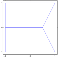
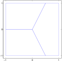
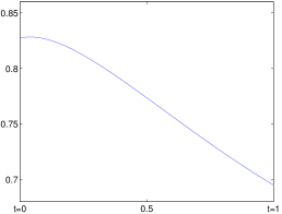
Figure 1. We consider a point set $P=\{q,p_{\pm}\}$, with $q=(2,0)$ and $p_{\pm}=(0,\pm 1)$, and a function $\varphi_{t}$ which linearly interpolates between $\varphi_{0}=\chi_{\{q\}}$ and $\varphi_{1}=0$. (Left) Laguerre cells $\operatorname{Lag}_{P}^{\varphi_{t}}(p)$ intersected with the square $[-1,1]^{2}$ at $t=0$. (Middle) Laguerre cells at $t=1$. (Right) Graph of the second moment of the measure $G_{\varphi_{t}{\#}}^{\mathrm{ac}}\mu$ as a function of $t$, showing the lack of convexity of a discretized energy.

Remark 3.2.

The convexity of the internal energy (3.33) also holds when considering the monotone discretization of the Monge-Ampère operator introduced by Oberman in [23].

Remark 3.3.

It seems necessary to consider two notions of push-forward of a given measure $\mu$. Indeed, the internal energy of a measure that is not absolutely continuous is $+\infty$, so that it only makes sense to compute the map $\mathcal{U}$ on the absolutely continuous measure $G_{\varphi\#}^{\mathrm{ac}}\mu$. On the other hand, condition (HE) is not sufficient to make the potential energy functional $\varphi\in\mathcal{K}^{G}_{Y}(P)\mapsto\mathcal{E}(G^{\mathrm{ac}}_{\varphi\#}\mu)$ convex. This can be seen on the example given in Figure 1: let $Y=[-1,1]^{2}$ and $P=\{q,p_{\pm}\}$ with $q=(2,0)$ and $p_{\pm}=(0,\pm 1)$. We let $\varphi_{t}$ be the linear interpolation between $\varphi_{0}:=\mathbf{1}_{\{q\}}$, and $\varphi_{1}=0$, and We let $\mu=0.8\delta_{q}+0.1\delta_{p_{+}}+0.1\delta_{p_{-}}$. The third column of Figure 1 displays the graph of the second moment of the absolutely continuous push-forward, i.e.

$$t\mapsto\mathcal{E}(G_{\varphi_{t}\#}^{\mathrm{ac}}\mu),\hbox{ where }\mathcal{E}(\nu)=\int_{\mathbb{R}^{d}}\left\|x\right\|^{2}\operatorname{d}\nu(x),$$ (3.35)

The graph shows that this function is not convex in $t$, even though $\mathcal{E}$ is convex under generalized displacement since it satisfies McCann’s condition (HE).

Remark 3.4.

The two maps considered in the Theorem can be computed more explicitely:

$$\mathcal{E}(G_{\varphi\#}\mu) =\sum_{p\in P}\mu_{p}V(G_{\varphi}(p))+\sum_{p,q\in P}\mu_{p}\mu_{q}W(G_{\varphi(p)},G_{\varphi(q)})$$ (3.36)

$$\mathcal{U}(G^{\mathrm{ac}}_{\varphi\#}\mu) =\sum_{p\in P}U\left(\frac{\mu_{p}}{\operatorname{MA}_{Y}[\varphi](p)}\right)\operatorname{MA}_{Y}[\varphi](p)$$ (3.37)

In particular, when $\mathcal{U}$ is the negative entropy ($U(r)=r\log r$), one has:

$$\mathcal{U}(G^{\mathrm{ac}}_{\varphi\#}\mu)=-\sum_{p\in P}\mu_{p}\log(\operatorname{MA}_{Y}[\varphi](p)).$$ (3.38)

Consequently the internal energy term plays the role of a barrier for the constraint set $\mathcal{K}_{Y}(P)$, that is: if $\mathcal{U}(G^{\mathrm{ac}}_{\varphi\#}\mu)$ is finite, then $\varphi$ belongs to the interior of $\mathcal{K}_{Y}(P)$. The same behavior remains true if the function $U$ has super-linear growth at infinity. This enables us to extend $\mathcal{U}(G^{\mathrm{ac}}_{\varphi\#}\mu)$ to the whole space $\mathbb{R}^{P}$, by setting it to $+\infty$ when $\operatorname{MA}_{Y}[\varphi](p)=0$ for some $p\in P$.

4. A convergence theorem

Let $X,Y$ be two convex domains in $\mathbb{R}^{d}$, and $\mu$ be a probability measure on $X$ which is absolutely continuous with respect to the Lebesgue measure on $X$, and whose density $\rho$ is bounded from above and below: $\rho\in[r,1/r]$, with $r>0$. We are interested in the minimization problem

$$\min_{\nu\in\mathcal{P}(Y)}\mathcal{F}(\nu)=\min\{\mathcal{F}(\left.\nabla\varphi\right|_{\#}\mu);\varphi\in\mathcal{K}_{Y}\},$$ (4.39)

$$\hbox{where }\mathcal{F}(\nu):=\operatorname{W}_{2}^{2}(\mu,\nu)+\mathcal{E}(\nu)+\mathcal{U}(\nu),$$ (4.40)

and where the terms of the functional $\mathcal{F}$ satisfy the following assumptions:

• the energy $\mathcal{E}$ (resp $\mathcal{U}$) is weakly continuous (resp. lower semicontinuous) on $\mathcal{P}(Y)$;

• $\mathcal{U}$ is an internal energy, defined as in (1.10), where the integrand $U:\mathbb{R}\to\mathbb{R}$ is convex, $U(0)=0$ and $U$ has superlinear growth at infinity i.e. $\lim_{s\to\infty}s^{-1}U(s)=+\infty$.

Remark 4.1.

Note that the condition (C2) is different from McCann’s condition (HU) for the displacement convexity of an internal energy. Among the internal energies that satisfy both McCann’s conditions and (C1)–(C2), one can cite those that occur in the gradient flow formulation of the heat equation, where $U(r)=r\log r$, and of the porous medium equation, for which $U(r)=\frac{1}{m-1}r^{m},$ with $m>1$. The superlinear growth assumption in (C2) ensures that the internal energy acts as a barrier for the convexity constraint in the approximated problem (4.41).

Theorem 4.1 ($\Gamma$-convergence).

Assume (C1)– (C2). Let $\mu_{n}$ be a sequence of probability measures supported on finite subsets $P_{n}\subseteq X$, converging weakly to the probability density $\rho$, and consider the discretized problem

$$\min_{(\varphi,G_{\varphi})\in\mathcal{K}^{G}_{Y}(P_{n})}\operatorname{W}_{2}^{2}(\mu_{n},G_{\varphi_{n}\#}\mu_{n})+\mathcal{E}(G_{\varphi_{n}\#}\mu_{n})+\mathcal{U}(G_{\varphi_{n}\#}^{\mathrm{ac}}\mu_{n}).$$ (4.41)

Then, there exists a minimizer $\varphi_{n}$ of (4.41). Moreover, the sequence of absolutely continuous measure $\sigma_{n}:=G_{\varphi_{n}\#}^{\mathrm{ac}}\mu_{n}$ is a minimizing sequence for the problem (4.39). If $\mathcal{F}$ has a unique minimizer $\nu$ on $\mathcal{P}(Y)$, then $\sigma_{n}$ converges weakly to $\nu$.

Step 1.

There exists a minimizer to (4.41).

Proof.

Let $(\varphi_{n}^{k})_{k}$ be a minimizing sequence (which we can normalize by imposing $\varphi_{n}^{k}(p)=0$ at a fixed $p\in P_{n}$). Since $Y$ is bounded, we may assume that, up to some not relabeled subsequences $\varphi_{n}^{k}$ and $G_{\varphi_{n}^{k}}$ converge to some $(\varphi_{n},G_{\varphi_{n}})$. We can also assume that $\hat{\varphi}_{n}^{k}:=[\varphi_{n}^{k}]_{\mathcal{K}_{Y}}$ converges uniformly to $\hat{\varphi}_{n}=[\varphi_{n}]_{\mathcal{K}_{Y}}$. The convergence in the Wasserstein term and in $\mathcal{E}$ is then obvious, it remains to prove a liminf inequality for the discretized internal energy. First note that thanks to (C2), we also have that there is a $\nu>0$ such that $\operatorname{MA}_{Y}[\varphi_{n}^{k}](p)\geq\nu$ for every $k$ and every $p\in P_{n}$. Then observe that the internal energy can be written as

$$\mathcal{U}(G_{\varphi_{n}^{k}\#}^{\mathrm{ac}}\mu_{n}):=\sum_{p\in P_{n}}F(p,\operatorname{MA}_{Y}[\varphi_{n}^{k}](p)),\;F(p,t):=tU\left(\frac{\mu_{p}}{t}\right)$$

so that $F(p,.)$ is nonincreasing thanks to (C2). It is then enough to prove that for every $p\in P_{n}$ one has:

$$\limsup_{k}\operatorname{MA}_{Y}[\varphi_{n}^{k}](p)=\limsup_{k}\mathcal{H}^{d}(\partial\hat{\varphi}_{n}^{k}(p))\leq\mathcal{H}^{d}(\partial\hat{\varphi}_{n}(p))$$ (4.42)

but the latter inequality follows at once from Fatou’s Lemma and the fact that if $y$ belongs to $\partial\hat{\varphi}_{n}^{k}(p)$ for infinitely many $k$ then it also necessarily belongs to $\partial\hat{\varphi}_{n}(p)$. This proves that $\varphi_{n}$ solves (4.41). ∎

Let $m$ and $m_{n}$ be the minima of (4.39) and (4.41) respectively. Our goal now is to show that $\lim_{n\to\infty}m_{n}=m$. In order to simplify the proof, we will keep the same notation for an absolutely continuous probability measure and its density.

Step 2.

$\lim\inf_{n\to\infty}m_{n}\geqslant m$

Proof.

For every $n$, let $\varphi_{n}\in\mathcal{K}_{Y}(P_{n})$ be a minimizer of the discretized problem (4.41). By compactness of the set $\mathcal{K}_{Y}$ (up to an additive constant), and taking a subsequence if necessary, we can assume that $\hat{\varphi}_{n}:=[\varphi_{n}]_{\mathcal{K}_{Y}}$ converges uniformly to a function $\varphi$ in $\mathcal{K}_{Y}$. We can also assume that both sequence of measures $\sigma_{n}:=G_{\varphi_{n}\#}^{\mathrm{ac}}\mu_{n}$ and $\nu_{n}:=G_{\varphi_{n}\#}\mu_{n}$ converge to two measures $\sigma$ and $\nu$ for the Wasserstein distance. The difficulty is to show that these two measures $\nu$ and $\sigma$ must coincide. Indeed, let $\pi_{n}$ (resp. $\pi_{n}^{\prime}$) be optimal transport plans between $\mu_{n}$ and $\nu_{n}$ (resp. $\mu_{n}$ and $\sigma_{n}$). Taking subsequences if necessary, these optimal transport plans converge to two transport plans $\pi$ (resp. $\pi^{\prime}$) between $\rho$ and $\nu$ (resp. $\rho$ and $\sigma$) that are supported on the graph of the gradient of $\varphi$. Since the first marginal of $\pi$ and $\pi^{\prime}$ coincide, one must have $\pi=\pi^{\prime}$ and therefore $\nu=\sigma$. The result then follows from the weak lower semicontinuity of $\mathcal{U}$, and the continuity of $(\mu,\nu)\mapsto\operatorname{W}_{2}^{2}(\mu,\nu)+\mathcal{E}(\nu)$. ∎

We now proceed to the proof that $\lim\sup_{n\to\infty}m_{n}\leqslant m$. Our first step is to show that probability measures with a smooth density bounded from below and above are dense in energy. More precisely, we have:

Step 3.

$m=\min_{\varepsilon>0}\min\{\mathcal{F}(\sigma);\sigma\in\mathcal{P}^{\mathrm{ac}}(Y)\cap\mathcal{C}^{0}(Y),\varepsilon\leqslant\sigma\leqslant 1/\varepsilon\}$

Proof.

Let $\sigma$ be a probability density on $Y$ such that $\mathcal{F}(\sigma)<+\infty$. Then, according to Corollary 1.4.3 in [2], there exists a sequence of probability densities $\sigma_{n}$ on $Y$ that satisfy the three properties:

• For every $n>0$, $\sigma_{n}$ is bounded from above and below:

  $$0<\inf_{y\in Y}\sigma_{n}(y)<\sup_{y\in Y}\sigma_{n}(y)<+\infty;$$

• $\sigma_{n}$ converges to $\sigma$ in $\mathrm{L}^{1}(Y)$;

• $\mathcal{U}(\sigma_{n})\leqslant\mathcal{U}(\sigma)$.

Moreover the proof of Corollary 1.4.3 in [2] can be modified by taking a smooth convolution operator so as to ensure that each $\sigma_{n}$ is continuous on $Y$. Our task is then to show that

$$\lim\inf_{n\to\infty}\mathcal{F}(\sigma_{n})\leqslant\mathcal{F}(\sigma),$$

where $\mathcal{F}(\sigma)=\operatorname{W}^{2}_{2}(\mu,\sigma)+\mathcal{E}(\sigma)+\mathcal{U}(\sigma)$. Thanks to (C1), and thanks to the Wasserstein continuity of the terms $\sigma\mapsto\operatorname{W}^{2}_{2}(\mu,\sigma)+\mathcal{E}(\sigma)$, we only need to show that $\sigma_{n}$ converges to $\sigma$ in the Wasserstein sense. This follows from the easy inequality

$$\operatorname{W}^{2}_{2}(\sigma,\sigma^{\prime})\leqslant\left\|\sigma-\sigma^{\prime}\right\|_{\mathrm{L}^{1}(Y)}\operatorname{diam}(Y)^{2}.\qed$$

Step 4.

Let $\sigma\in\mathcal{P}(Y)\cap\mathcal{C}^{0}(Y)$, with $\varepsilon\leqslant\sigma\leqslant 1/\varepsilon$. Then, for every $n\geqslant 0$, there exists a convex interpolate $\varphi_{n}\in\mathcal{K}_{Y}(P_{n})$ such that

$$\forall p\in P_{n},~{}\sigma(\partial[\varphi_{n}]_{\mathcal{K}_{Y}}(p))=\mu_{n}(\{p\}).$$ (4.43)

Proof.

By Breniers’ theorem, there is a convex potential $\psi_{n}$ on $Y$ such that $\nabla\psi_{n}\#\sigma=\mu_{n}$, so that $\varphi_{n}:=\psi_{n}^{*}$ has the desired property. ∎

Step 5.

Assuming that the functions $\varphi_{n}$ in $\mathcal{K}_{Y}(P_{n})$ are constructed as above, we can bound the diameter of their subdifferentials:

$$\lim_{n\to\infty}\max_{p\in P_{n}}\operatorname{diam}(\partial[\varphi_{n}]_{\mathcal{K}_{Y}}(p))=0.$$ (4.44)

Proof.

Let $\hat{\varphi}\in\mathcal{K}_{Y}$ be a potential for the quadratic optimal transport problem between $\rho$ and $\sigma$. Let $\hat{\varphi}_{n}:=[\varphi_{n}]_{\mathcal{K}_{Y}}$ and $\psi=\hat{\varphi}^{*}$ and $\psi_{n}=\hat{\varphi}_{n}^{*}$. First, we add a constant to $\varphi$ and $\varphi_{n}$ such that the integral of $\psi$ and $\psi_{n}$ over $\sigma$ is zero,

$$\int_{Y}\psi(y)\sigma(y)\operatorname{d}y=\int_{Y}\psi_{n}(y)\sigma(y)\operatorname{d}y=0.$$

Poincaré’s inequality on $Y$ with density $\sigma$ gives us

$$\int_{Y}\left|\psi_{n}(y)-\psi(y)\right|^{2}\sigma(y)\operatorname{d}y \leqslant\mathrm{const}(p,Y,\sigma)\int_{Y}\left\|\nabla\psi_{n}-\nabla\psi(y)\right\|^{2}\sigma(y)\operatorname{d}y,$$

and the weak continuity of optimal transport plans then ensures that the right-hand term converges to zero. Noting that $\psi_{n}$ and $\psi$ are convex on $Y$ and have a bounded Lipschitz constant, because the gradients $\nabla\psi,\nabla\psi_{n}$ belong to $X$, this implies that $\psi_{n}$ converge uniformly to $\psi$. Taking the Legendre transform, this shows that $\hat{\varphi}_{n}$ converges uniformly to $\hat{\varphi}$ on the compact domain $X$.

We now prove (4.44) by contradiction, and we assume that there exists a positive constant $r$, and a sequence of points $(p_{n})$, with $p_{n}\in P_{n}$ and such that there exists $y_{n},y_{n}^{\prime}\in\partial\hat{\varphi}_{n}$ with $\left\|y_{n}-y_{n}^{\prime}\right\|\geqslant r$. By compactness, and taking subsequences if necessary, we can assume that $p_{n}$ converges to a point $p$ in $X$ and that the sequences $(y_{n})$ and $(y_{n}^{\prime})$ converge to two points $y,y^{\prime}$ in $Y$ with $\left\|y-y^{\prime}\right\|\geqslant r$. Since the point $y_{n}$ belongs to $\partial\hat{\varphi}_{n}(p_{n})$, one has:

$$\forall x\in X,~{}\hat{\varphi}_{n}(x)\geqslant\hat{\varphi}_{n}(p_{n})+\langle y_{n}|x-p\rangle.$$

Taking the limit as $n$ goes to $\infty$, this shows us that $y$ (and similarly $y^{\prime}$) belongs to $\partial\hat{\varphi}(p)$, so that $\operatorname{diam}(\partial\hat{\varphi}(p))\geqslant r$. The contradiction then follows from Caffarelli’s regularity result [10]: under the assumptions on the supports and on the densities, the map $\hat{\varphi}$ is $\mathcal{C}^{1,\beta}$ up to the boundary of $X$. In particular, the subdifferential of $\hat{\varphi}$ must be a singleton at every point of $X$, thus contradicting the lower bound on its radius. ∎

Step 6.

Let $\sigma_{n}:=G_{\varphi_{n}\#}^{\mathrm{ac}}\mu_{n}$ and $\nu_{n}:=G_{\varphi_{n}\#}\mu_{n}$, where $\varphi_{n}$ is defined above. Then,

$$\lim_{n\to\infty}\left\|\sigma_{n}-\sigma\right\|_{\mathrm{L}^{\infty}(Y)}=0.$$ (4.45)

$$\lim_{n\to\infty}\operatorname{W}_{2}(\nu_{n},\sigma)=0.$$ (4.46)

Proof.

First, note that since $\sigma$ is continuous on a compact set, it is also uniformly continuous. For any $\delta>0$, there exists $\varepsilon>0$ such that $\left\|x-y\right\|\leqslant\varepsilon$ implies $\left|\sigma(x)-\sigma(y)\right|\leqslant\delta$. Using Equation (4.44), for $n$ large enough, the sets $V_{p}:=\partial[\varphi_{n}]_{\mathcal{K}_{Y}}(p)$ have diameter bounded by $\varepsilon$ for all point $p$ in $P_{n}$. By definition, the density $\sigma_{n}$ is equal to

$$\sigma_{n}=\sum_{p\in P}\hat{\sigma}_{p}\chi_{V_{p}}\hbox{ with }\hat{\sigma}_{p}:=\frac{1}{\mathcal{H}^{d}(V_{p})}\int_{V_{p}}\sigma(x)\operatorname{d}x.$$ (4.47)

By the uniform continuity property, on every cell $V_{p}$ one has $\left|\sigma(x)-\hat{\sigma}_{p}\right|\leqslant\delta$, thus proving $\left\|\sigma_{n}-\sigma\right\|_{\mathrm{L}^{\infty}(Y)}\leqslant\delta$ for $n$ large enough. This implies that $\sigma_{n}$ converges to $\sigma$ uniformly, and a fortiori that $\lim_{n\to\infty}\operatorname{W}_{2}(\sigma_{n},\sigma)=0$. Then,

$$\operatorname{W}_{2}(\nu_{n},\sigma)\leqslant\operatorname{W}_{2}(\nu_{n},\sigma_{n})+\operatorname{W}_{2}(\sigma_{n},\sigma).$$ (4.48)

Moreover, one can bound the Wasserstein distance explicitely between $\sigma_{n}$ and $\nu_{n}$ by considering the obvious transport plan on each of the subdifferentials $(\partial[\varphi_{n}]_{\mathcal{K}_{Y}}(p))_{p\in P_{n}}$:

$$\operatorname{W}^{2}_{2}(\nu_{n},\sigma_{n})\leqslant\sum_{p\in P_{n}}\operatorname{diam}(\partial[\varphi_{n}]_{\mathcal{K}_{Y}}(p))\mu_{p}\leqslant\max_{p\in P_{n}}\operatorname{diam}(\partial[\varphi_{n}]_{\mathcal{K}_{Y}}(p)).$$ (4.49)

The second statement (4.46) follows from Eqs. (4.48), (4.49) and (4.44). ∎

Step 7.

$\lim_{n\to\infty}\operatorname{W}_{2}^{2}(\mu_{n},\nu_{n})+\mathcal{E}(\nu_{n})+\mathcal{U}(\sigma_{n})=\operatorname{W}_{2}^{2}(\mu,\sigma)+\mathcal{E}(\sigma)+\mathcal{U}(\sigma)$

Proof.

The convergence of the first two terms follows from the Wasserstein continuity of the map $(\mu,\nu)\in\mathcal{P}(Y)\mapsto\operatorname{W}_{2}^{2}(\mu,\nu)+\mathcal{E}(\nu)$. In order to deal with the third term, we will assume that $n$ is large enough, so that the densities $\sigma,\sigma_{n}$ belong to the segment $S_{\varepsilon/2}=[\varepsilon/2,2/\varepsilon]$. The integrand $U$ of the internal energy is convex on $\mathbb{R}$, and therefore Lipschitz with constant $L$ on $S_{\varepsilon/2}$, so that

$$\left|\int_{Y}U(\sigma_{n})\operatorname{d}x-\int_{Y}U(\sigma(x))\operatorname{d}x\right| \leqslant\int_{Y}\left|U(\sigma_{n})-U(\sigma(x))\right|\operatorname{d}x$$

$$\leqslant L\left\|\sigma_{n}-\sigma\right\|_{\mathrm{L}^{\infty}(Y)}.\qed$$

5. Numerical results

5.1. Computation of the Monge-Ampère operator

In this paragraph we explain how to evaluate the discretized internal energy of $G_{\varphi\#}^{\mathrm{ac}}\mu_{P}$, where $\varphi$ is a discrete convex function in $\mathcal{K}_{Y}(P)$, and $Y$ is a polygon in the euclidean plane. Thanks to the equation

$$\mathcal{U}(G_{\varphi\#}^{\mathrm{ac}}\mu_{P})=\sum_{p\in P}U\left(\mu_{p}/\operatorname{MA}_{Y}[\varphi](p)\right)\operatorname{MA}_{Y}[\varphi](p),$$ (5.50)

one can see that the internal energy and its first and second derivatives can be easily computed if one knows how to evaluate the discrete Monge-Ampère operator and its derivatives with respect to $\varphi$. Our assumptions for performing this computation will be the following:

• the domain $Y$ is a convex polygon and its boundary can be decomposed as a finite union of segments $S=\{s_{1},\ldots,s_{k}\}$

• the points in $P$ are in generic position, i.e. (a) there does not exist a triple of collinear points in $P$ and (b) for any pair $p,q$ of distinct points in $P$, there is no segment $s$ in $S$ which is collinear to the bisector of $[pq]$.

The Jacobian matrix of the discrete Monge-Ampère operator is a square matrix denoted $(\operatorname{JMA}_{Y}[\varphi])_{p,q\in P}$, while its Hessian is a $3$-tensor denoted $(\operatorname{HMA}_{Y}[\varphi])_{p,q,r\in P}$. The entries of this matrix and tensor are given by the formulas

$$\operatorname{JMA}_{Y}[\varphi]_{pq} :=\frac{\partial\operatorname{MA}_{Y}[\varphi](p)}{\partial\mathbf{1}_{q}},$$ (5.51)

$$\operatorname{HMA}_{Y}[\varphi]_{pqr} :=\frac{\partial^{2}\operatorname{MA}_{Y}[\varphi](p)}{\partial\mathbf{1}_{r}\partial\mathbf{1}_{q}},$$ (5.52)

where $\mathbf{1}_{p}$ denotes the indicator function of a point $p$ in $P$. The goal of the remaining of this section is to show how the computation of the Jacobian matrix and the Hessian tensor are related to a triangulation which is defined from the Laguerre cells by duality.

Abstract dual triangulation

Given any function $\varphi$ on $P$, we introduce a notation for the intersection of the Laguerre cell of $P$ with $Y$, and we extend this notation to handle boundary segments as well. More precisely, we set:

$$\forall p\in P,~{}V^{\varphi}(p) :=\operatorname{Lag}_{P}^{\varphi}(p)\cap Y,$$ (5.53)

$$\forall s\in S,~{}V^{\varphi}(s) :=s.$$

We also introduce a notation for the finite intersections of these cells:

$$\forall p_{1},\ldots,p_{s}\in P\cup S,~{}V^{\varphi}(p_{1}\ldots p_{s}):=V^{\varphi}(p_{1})\cap...\cap V^{\varphi}(p_{s})$$ (5.54)

The decomposition of $Y$ given by the cells $V^{\varphi}(p)$ induces an abstract dual triangulation $T^{\varphi}$ of the set $P\cup S$, whose triangles and edges are characterized by:

• a pair $(p,q)$ in $P\cup S$ is an edge of $T^{\varphi}$ iff $V^{\varphi}(pq)\neq\emptyset$;

• a triplet $(p,q,r)$ in $P\cup S$ is a triangle of $T^{\varphi}$ iff $V^{\varphi}(pqr)\neq\emptyset$.

An example of such an abstract dual triangulation is displayed in Figure 2.

The construction of this triangulation can be performed in time $\mathrm{O}(N\log N+k)$, where $N$ is the number of points and $k$ is the number of segments in the boundary of $Y$. The construction works by adapting the regular triangulation of the point set, which is the triangulation obtained when $Y=\mathbb{R}^{d}$, and for which there exists many algorithms, see e.g. [1].

Jacobian of the Monge-Ampère operator

By Lemma 2.3, for any point $p$ in $P$, the function $\varphi\mapsto\operatorname{MA}_{Y}[\varphi](p)$ is log-concave on the set $\mathcal{K}_{Y}(P)$. This function is therefore twice differentiable almost everywhere on the interior of $\mathcal{K}_{Y}(P)$, using Alexandrov’s theorem. The first derivatives of the Monge-Ampère operator is easy to compute, and involves boundary terms: two points $p,q$ in $P$,

$$\operatorname{JMA}_{Y}[\varphi]_{pq} =\frac{\mathcal{H}^{1}(V^{\varphi}(pq))}{\left\|p-q\right\|}\hbox{ if }q\neq p$$ (5.55)

$$\operatorname{JMA}_{Y}[\varphi]_{pq} =-\sum_{\begin{subarray}{c}q\in P\\ (qp)\in T^{\varphi}\end{subarray}}\frac{\mathcal{H}^{1}(V^{\varphi}(pq))}{\left\|p-q\right\|}$$ (5.56)

Note that every non-zero element in the square matrix corresponds to an edge in the dual triangulation $T^{\varphi}$.

Hessian of the Monge-Ampère operator

We will not include the computation of the second order derivatives, but we will sketch how it can be performed using the triangulation $T^{\varphi}$. First, we remark that thanks to our genericity assumption, for every triangle $pqr$ of $T^{\varphi}$, the set $V^{\varphi}(pqr)$ consists of a single point, which we also denote $V^{\varphi}(pqr)$. For any edge $pq$ in the triangulation $T^{\varphi}$, where $p,q$ are two points in $P$, the intersection $V^{\varphi}(pq)=V^{\varphi}(q)\cap V^{\varphi}(q)$ is a segment $[x,y]$. The endpoint $x$ of this segment needs to be contained in a third cell $V^{\varphi}(r)$ for a certain element $r$ of $P\cup S\setminus\{p,q\}$, so that $x=V^{\varphi}(pqr)$. Similarly, there exists $r^{\prime}$ in $P\cup S\setminus\{p,q\}$ such that $y=V^{\varphi}(pqr^{\prime})$. One can therefore rewrite the length of $V^{\varphi}(pq)$ as

$$\mathcal{H}^{1}(V^{\varphi}(pq))=\left\|V^{\varphi}(pqr)-V^{\varphi}(pqr^{\prime})\right\|.$$ (5.57)

The expression of the Hessian can be deduced from Equations (5.55)–(5.56) and (5.57), and from an explicit computation for the point $V^{\varphi}(pqr)$. Moreover, to each nonzero element of the Hessian one can associate a point, an edge or a triangle in the triangulation $T^{\varphi}$. More precisely:

$$\operatorname{HMA}_{Y}[\varphi]_{pqr}\neq 0\Longrightarrow p=q=r \hbox{ or }(p=q\hbox{ and }(pr)\hbox{ is an edge of }T^{\varphi})$$

$$\hbox{ or }(pqr)\hbox{ is a triangle of }T^{\varphi}.$$

In particular, the total number of non-zero elements of the tensor $\operatorname{HMA}_{Y}[\varphi]$ is at most proportional to the number $\left|P\right|$ of points plus the number $\left|S\right|$ of segments.

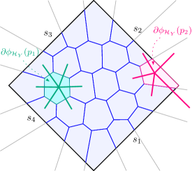
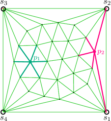
Figure 2. On the left, the intersection of power cells with a convex polygon (in red), and on the right, the dual triangulation.

5.2. Non-linear diffusion on point clouds

The first application is non-linear diffusion in a bounded convex domain $X$ in the plane. We are interested in the following PDE, where the parameter $m$ is chosen in $[1-1/d,+\infty)$. A numerical application is displayed on Figure 3 .

$$\left\{\begin{aligned} \frac{\partial\rho}{\partial t}&=\Delta\rho^{m}&\hbox{on }X\\ \nabla\rho&\perp\mathbf{n}_{X}&\hbox{on }\partial X\end{aligned}\right.$$ (5.58)

When $m=1$, this PDE is the classical heat equation with Neumann boundary conditions. When $m<1$, this PDE provides a model of fast dixffusion, while for $m>1$ it is a model for the evolution of gases in a porous medium. Otto [25] reinterpreted this PDE as a gradient flow in the Wasserstein space for the internal energy

$$\mathcal{U}_{m}(\mu)=\left\{\begin{aligned} &\int_{\mathbb{R}^{d}}U_{m}(\rho(x))\operatorname{d}x\hbox{ if }\mu\ll\mathcal{H}^{d},\rho:=\frac{\operatorname{d}\mu}{\operatorname{d}\mathcal{H}^{d}},\\ &+\infty\hbox{ if not.}\end{aligned}\right.,$$ (5.59)

where $U_{m}(r)=\frac{r^{m}(x)}{m-1}$ when $m\neq 1$ and $U_{1}(r)=r\log r$. A time-discretization of this gradient-flow model can be defined using the Jordan-Kinderlehrer-Otto scheme: given a timestep $\tau>0$ and a probability measure $\mu_{0}$ supported on $X$, one defines a sequence of probability measures $(\mu_{k})_{k\geqslant 1}$ recursively

$$\mu_{k+1}=\arg\min_{\mu\in\mathcal{P}(X)}\operatorname{W}_{2}^{2}(\mu_{k},\mu)+\mathcal{U}_{m}(\mu)$$ (5.60)

The energies involved in this optimization problem satisfy McCann’s assumption for displacement convexity, and our discrete framework is therefore able to provide a discretization in space of Equation (5.60) as a convex optimization problem. We use this discretization in order to construct the non-linear diffusion for a finite point set $P_{0}$ contained in the convex domain $X$. Note that for this experiment, we do not use the formulation involving the space of convex interpolates with gradient, $\mathcal{K}_{X}^{G}(P)$. For every function $\varphi$ in $\mathcal{K}_{Y}(P)$, and every point $p$ in $P$, we select explicitely a subgradient in the subdifferential $\partial\varphi_{\mathcal{K}_{Y}}(p)$ by taking its Steiner point [26].

We start with $\mu_{0}=\sum_{p\in P}\delta_{p}/\left|P\right|$ the uniform measure on the set $P_{0}$, and we define recursively

$$\left\{\begin{aligned} &\varphi_{k}=\arg\min\left\{\frac{1}{2\tau}\operatorname{W}^{2}_{2}(\mu_{k},G_{\varphi\#}\mu_{k})+\mathcal{U}(G_{\varphi\#}^{\mathrm{ac}}\mu_{k});\varphi\in\mathcal{K}_{X}(P_{k})\right\}\\ &\mu_{k+1}=G_{\varphi_{k}\#}\mu_{k},\\ &P_{k+1}=\mathrm{spt}(\mu_{k+1})\end{aligned}\right.,$$ (5.61)

where $G_{\varphi}(p)$ is the Steiner point of $\partial\varphi_{\mathcal{K}_{Y}}(p)$. This minimization problem is solved using a second-order Newton method. Note that, as mentioned in the remark following Theorem 3.1, the internal energy plays the role of a barrier for the convexity of the discrete function $\varphi$. When second-order methods fail, one could also resort to more robust first-order methods for the resolution of the optimization problem, using for instance a projected gradient algorithm.

Figure 3. (Top) The original point set $P_{0}$ in the square domain $X=[-2,2]^{2}$ contains 2 900 points. (Bottom rows) The evolution of the point cloud $P_{k}$ at timesteps $k=5,10,20,40,80$ with $\tau=0.01$ is defined using Eq. (5.61) for various values of the exponent $m$. From top to bottom, $m$ takes increasing values in $\{0.6,1,2,3\}$. Note that the case $m=0.6$ is outside of the scope of the $\Gamma$-convergence theorem

5.3. Crowd-motion with congestion

As a second application, we consider the model of crowd motion with congestion introduced by Maury, Roudneff-Chupin and Santambrogio [19]. The crowd is represented by a probability density $\mu_{0}$ on a convex compact subset with nonempty interior $X$ of $\mathbb{R}^{2}$, which is bounded by a certain constant, which we assume normalized to one (so that we also naturally assume that $\mathcal{H}^{d}(X)>1$). One is also given a potential $V:X\to\mathbb{R}$, which we assume to be $\lambda$-convex, i.e. $V(.)+\lambda\left\|.\right\|^{2}$ is convex. The evolution of the probability density describing the crowd is induced by the gradient flow of the potential energy

$$\mathcal{E}(\mu)=\int_{\mathbb{R}^{d}}V(x)\operatorname{d}\mu(x),$$ (5.62)

in the Wasserstein space, under the additional constraint that the density needs to remain bounded by one. We rely again on time-discretization of this gradient flow using the Jordan-Kinderlehrer-Otto scheme. This gives us the following formulation:

$$\mu_{k+1}=\arg\min_{\mu\in\mathcal{P}(X)}\frac{1}{2\tau}\operatorname{W}_{2}^{2}(\mu_{k},\mu)+\mathcal{E}(\mu)+\mathcal{U}(\mu),$$ (5.63)

where $\mathcal{U}$ is the indicatrix function of the probability measures whose density is bounded by one:

$$\mathcal{U}(\mu)=\left\{\begin{aligned} &0\hbox{ if }\mu\ll\mathcal{H}^{d}\hbox{ and }\frac{\operatorname{d}\mu}{\operatorname{d}\mathcal{H}^{d}}\leqslant 1\\ &+\infty\hbox{ if not.}\end{aligned}\right.$$ (5.64)

In order to perform numerical simulations, we replace this indicatrix function by a smooth approximation.

$$\mathcal{U}_{\alpha}(\mu)=\left\{\begin{aligned} &\int_{\mathbb{R}^{d}}\rho^{\alpha}(x)(-\log(1-\rho(x)^{1/d})\operatorname{d}x\hbox{ if }\mu\ll\mathcal{H}^{d}\hbox{ and }\rho:=\frac{\operatorname{d}\mu}{\operatorname{d}\mathcal{H}^{d}},\\ &+\infty\hbox{ if not.}\end{aligned}\right.$$ (5.65)

Note that if $\mathcal{U}_{\alpha}(\mu)$ is finite, then the density of $\mu$ is bounded by one almost everywhere. Moreover, we have the following convexity and $\Gamma$-convergence results:

Proposition 5.1.

• The energy $\mathcal{U}_{\alpha}$ is convex under general displacement.

• $\mathcal{U}_{\alpha}$ $\Gamma$-converges (for the weak convergence of measures on $X$) to $\mathcal{U}$ as $\alpha$ tends to $+\infty$ ;

• $\beta\mathcal{U}_{1}$ $\Gamma$-converges to $\mathcal{U}$ as $\beta$ tends to $0$.

Proof.

The proof of (i) uses McCann’s theorem: one only needs $r^{d}U(r^{-d})$ to be convex non-increasing and $U(0)=0$, which follows from a simple computation. (ii) The proof of the $\Gamma$-liminf inequality is obvious since $\mathcal{U}_{\alpha}\geq\mathcal{U}$ and $\mathcal{U}$ is lower semicontinuous. As for the $\Gamma$-limsup inequality, we proceed as follows: we first fix $\mu\in\mathcal{P}(X)$ such that $\mathcal{U}(\mu)=0$ (otherwise, there is nothing to prove). Let us then fix a set $A\subset X$ such that $\mathcal{H}^{d}(A)>1$ and let $m$ be the uniform probability measure on $A$. For $\varepsilon\in(0,1)$, let us then define $\mu_{\varepsilon}:=(1-\varepsilon)\mu+\varepsilon m$ so that $\mu_{\varepsilon}$ has a density bounded by $1-C\varepsilon$ where $C:=1-\frac{1}{\mathcal{H}^{d}(A)}>0$. Letting $\alpha\to\infty$ and setting $\varepsilon_{\alpha}\sim\alpha^{-1/2}$, one directly checks that $\limsup_{\alpha}\mathcal{U}_{\alpha}(\mu_{\varepsilon_{\alpha}})=O(e^{-\alpha^{1/2}}\log(\alpha))=0=\mathcal{U}(\mu)$ which proves the $\Gamma$-limsup inequality. For (iii), the proof is similar, choosing $\varepsilon_{\beta}\sim e^{-\beta^{-1/2}}$ as $\beta\to 0$ for the $\Gamma$-limsup inequality. ∎

Numerical result

Figure 4 displays a numerical application, where we compute the Wasserstein gradient flow of a probability density whose energy is given by

$$\mathcal{F}(\rho)=\int_{X}V(x)\rho(x)\operatorname{d}x+\alpha\mathcal{U}_{1}(\rho),$$ (5.66)

$$\hbox{where }X=[-2,2]^{2},~{}\hbox{ and }V(x)=\left\|x-(2,0)\right\|^{2}+5\exp(-5\left\|x\right\|^{2}/2).$$

Note that the chosen potential is semi-convex. We track the evolution of a probability density on a fixed grid, which allows us to use a simple finite difference scheme to evaluate the gradient of the transport potential. From one timestep to another, the mass of the absolutely continuous pushforward of the minimizer is redistributed on the fixed grid.

Figure 4. Simulation of crowd motion under congestion using the gradient flow formulation. The congestion term is given by $\beta\mathcal{U}_{1}$ (see Equation (5.65)), for various values of $\beta$. From top to bottom, $\beta$ is set to $10^{-k}$ for $0\leqslant k\leqslant 2$.

Acknowledgements.

The authors gratefully acknowledge the support of the French ANR, through the projects ISOTACE (ANR-12-MONU-0013), OPTIFORM (ANR-12-BS01-0007) and TOMMI (ANR-11-BSO1-014-01).

References

- [1] Cgal, Computational Geometry Algorithms Library, http://www.cgal.org.
- [2] Martial Agueh, Existence of solutions to degenerate parabolic equations via the monge-kantorovich theory., Ph.D. thesis, Georgia Institute of Technology, USA, 2002.
- [3] by same author, Existence of solutions to degenerate parabolic equations via the monge-kantorovich theory, Advances in Differential Equations 10 (2005), no. 3, 309–360.
- [4] Martial Agueh and Malcolm Bowles, One-dimensional numerical algorithms for gradient flows in the p-wasserstein spaces, Acta applicandae mathematicae 125 (2013), no. 1, 121–134.
- [5] Luigi Ambrosio, Nicola Gigli, and Giuseppe Savaré, Gradient flows: in metric spaces and in the space of probability measures, Lectures in Mathematics ETH Zürich (2005).
- [6] Adrien Blanchet, Vincent Calvez, and José A Carrillo, Convergence of the mass-transport steepest descent scheme for the subcritical patlak-keller-segel model, SIAM Journal on Numerical Analysis 46 (2008), no. 2, 691–721.
- [7] Adrien Blanchet and Guillaume Carlier, Optimal transport and cournot-nash equilibria, arXiv preprint arXiv:1206.6571 (2012).
- [8] Yann Brenier, Polar factorization and monotone rearrangement of vector-valued functions, Communications on pure and applied mathematics 44 (1991), no. 4, 375–417.
- [9] Martin Burger, Jose A Carrillo, Marie-Therese Wolfram, et al., A mixed finite element method for nonlinear diffusion equations, Kinetic and Related Models 3 (2010), no. 1, 59–83.
- [10] Luis A Caffarelli, Boundary regularity of maps with convex potentials, Communications on pure and applied mathematics 45 (1992), no. 9, 1141–1151.
- [11] Guillaume Carlier, Thomas Lachand-Robert, and Bertrand Maury, A numerical approach to variational problems subject to convexity constraint, Numerische Mathematik 88 (2001), no. 2, 299–318.
- [12] José A Carrillo and J Salvador Moll, Numerical simulation of diffusive and aggregation phenomena in nonlinear continuity equations by evolving diffeomorphisms, SIAM Journal on Scientific Computing 31 (2009), no. 6, 4305–4329.
- [13] Philippe Choné and Hervé VJ Le Meur, Non-convergence result for conformal approximation of variational problems subject to a convexity constraint, Numer. Funct. Anal. Optim. 5-6 (2001), no. 22, 529–547.
- [14] Ivar Ekeland and Santiago Moreno-Bromberg, An algorithm for computing solutions of variational problems with global convexity constraints, Numerische Mathematik 115 (2010), no. 1, 45–69.
- [15] Cristian E Gutiérrez, The Monge-Ampère equation, vol. 44, Birkhauser, 2001.
- [16] Richard Jordan, David Kinderlehrer, and Felix Otto, The variational formulation of the fokker–planck equation, SIAM journal on mathematical analysis 29 (1998), no. 1, 1–17.
- [17] David Kinderlehrer and Noel J Walkington, Approximation of parabolic equations using the wasserstein metric, ESAIM: Mathematical Modelling and Numerical Analysis 33 (1999), no. 04, 837–852.
- [18] Thomas Lachand-Robert and Édouard Oudet, Minimizing within convex bodies using a convex hull method, SIAM Journal on Optimization 16 (2005), no. 2, 368–379.
- [19] Bertrand Maury, Aude Roudneff-Chupin, and Filippo Santambrogio, A macroscopic crowd motion model of gradient flow type, Mathematical Models and Methods in Applied Sciences 20 (2010), no. 10, 1787–1821.
- [20] Robert J McCann, A convexity principle for interacting gases, Advances in Mathematics 128 (1997), no. 1, 153–179.
- [21] Quentin Mérigot and Edouard Oudet, Handling convexity-like constraints in variational problems, arXiv preprint arXiv:1403.2340 (2014).
- [22] Jean-Marie Mirebeau, Adaptive, anisotropic and hierarchical cones of discrete convex functions, arXiv preprint arXiv:1402.1561 (2014).
- [23] Adam M Oberman, Wide stencil finite difference schemes for the elliptic monge-ampere equation and functions of the eigenvalues of the hessian, Discrete Contin. Dyn. Syst. Ser. B 10 (2008), no. 1, 221–238.
- [24] by same author, A numerical method for variational problems with convexity constraints, SIAM Journal on Scientific Computing 35 (2013), no. 1, A378–A396.
- [25] Felix Otto, The geometry of dissipative evolution equations: the porous medium equation, Communications in partial differential equations 26 (2001), no. 1-2, 101–174.
- [26] Rolf Schneider, Convex bodies: the brunn-minkowski theory, vol. 44, Cambridge University Press, 1993.
- [27] Neil S. Trudinger and Xu-Jia Wang, The affine Plateau problem, J. Amer. Math. Soc. 18 (2005), no. 2, 253–289.
- [28] Bin Zhou, The first boundary value problem for Abreu’s equation, Int. Math. Res. Not. IMRN (2012), no. 7, 1439–1484.