The Approximate Loebl–Komlós–Sós Conjecture III:
The finer structure of LKS graphs

Abstract

This is the third of a series of four papers in which we prove the following relaxation of the Loebl–Komlós–Sós Conjecture: For every $\alpha>0$ there exists a number $k_{0}$ such that for every $k>k_{0}$ every $n$-vertex graph $G$ with at least $(\frac{1}{2}+\alpha)n$ vertices of degree at least $(1+\alpha)k$ contains each tree $T$ of order $k$ as a subgraph.

In the first paper of the series, we gave a decomposition of the graph $G$ into several parts of different characteristics. In the second paper, we found a combinatorial structure inside the decomposition. In this paper, we will give a refinement of this structure. In the forthcoming fourth paper, the refined structure will be used for embedding the tree $T$.

Mathematics Subject Classification: 05C35 (primary), 05C05 (secondary).
Keywords: extremal graph theory; Loebl–Komlós–Sós Conjecture; tree embedding; regularity lemma; sparse graph; graph decomposition.

1 Introduction

This is the third of a series of four papers [HKP⁺a, HKP⁺b, HKP⁺c, HKP⁺d] in which we provide an approximate solution of the Loebl–Komlós–Sós Conjecture. The conjecture reads as follows.

Conjecture 1.1 (Loebl–Komlós–Sós Conjecture 1995 [EFLS95]).

Suppose that $G$ is an $n$-vertex graph with at least $n/2$ vertices of degree more than $k-2$. Then $G$ contains each tree of order $k$.

We discuss the history and state of the art in detail in the first paper [HKP⁺a] of our series. The main result, which will be proved in [HKP⁺d], is the approximate solution of the Loebl–Komlós–Sós Conjecture, namely the following.

Theorem 1.2 (Main result [HKP⁺d]).

For every $\alpha>0$ there exists $k_{0}$ such that for any $k>k_{0}$ we have the following. Each $n$-vertex graph $G$ with at least $(\frac{1}{2}+\alpha)n$ vertices of degree at least $(1+\alpha)k$ contains each tree $T$ of order $k$.

In the first paper [HKP⁺a] we exposed the decomposition techniques, finding a sparse decomposition of the host graph $G$. The sparse decomposition should be thought of as a counterpart to the Szemerédi regularity lemma (but compared to the Szemerédi regularity lemma the sparse decomposition seems to be less versatile). In the second paper [HKP⁺b], we combined the sparse decomposition with a matching structure, obtaining in [HKP⁺b, Lemma LABEL:p1.prop:LKSstruct] what we call the rough structure. The rough structure obtained in [HKP⁺b, Lemma LABEL:p1.prop:LKSstruct] depends on the graph $G$ only, i.e., is independent of the tree $T$. The rough structure encodes the general information how $T$ should be embedded on a macroscopic scale. However, from the perspective of embedding small parts of $T$ locally, the properties of the rough structure are insufficient. In the present paper we take the preparation of the host graph one step further, refining the rough structure. This way we obtain one of ten possible configurations. Formally, each of the configuration — denoted by $\mathbf{(\diamond 1)}$–$\mathbf{(\diamond 10)}$ — is a collection of favourable properties the said graph must satisfy. Each of these configurations is based on the building blocks of the sparse decomposition, and describes in a very fine way a substructure in $G$. Some of the configurations involve some basic parameters of the tree $T$. That is, while the presence of some individual configurations (namely, configuration $\mathbf{(\diamond 1)}$–$\mathbf{(\diamond 5)}$ and $\mathbf{(\diamond 10)}$ introduced in Section 3) suffices for embedding of each $k$-vertex tree, configurations $\mathbf{(\diamond 6)}$–$\mathbf{(\diamond 9)}$ are accompanied by parameters (denoted by $h$, $h_{1}$ and $h_{2}$ in Definitions 4.11–4.14) that depend on certain parameters of the tree $T$.

In the last paper [HKP⁺d] we will prove that each of these ten configurations allows to embed $T$. This will complete the proof of Theorem 1.2. An overview of how the embedding goes for each individual configuration is given in [HKP⁺d, Section LABEL:p3.ssec:embeddingOverview]. We recommend the reader to consult this part of [HKP⁺d] in parallel when reading through the definitions of the configurations in Section 4.

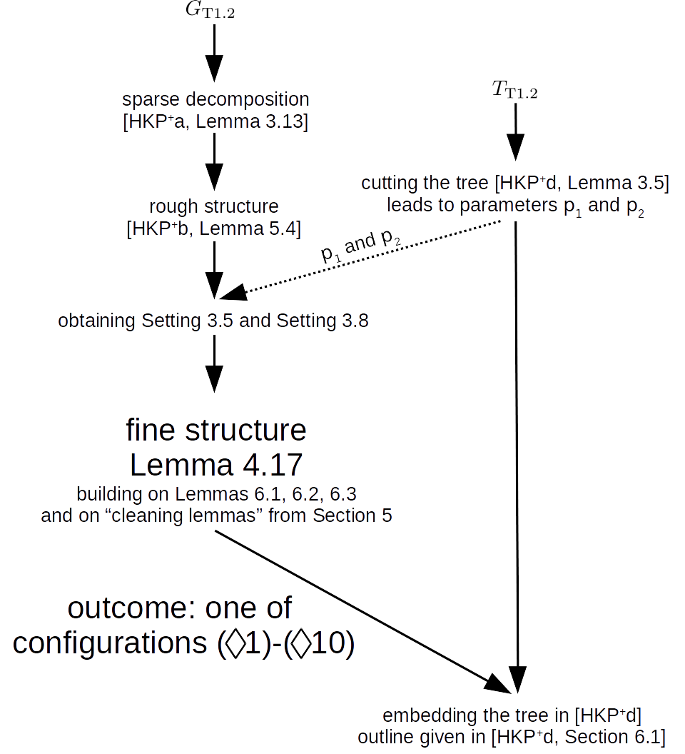
Figure 1.1: Diagram of the proof of Theorem 1.2 with focus on the part dealt with in this paper.

The paper is organized as follows. In Section 2 we introduce some basic notation. In Section 3 we introduce some further auxiliary notions, and two “settings” that will be common to the rest of the paper. In Section 4, we present the main result of this paper, Lemma 4.17. The lemma says that in any graph that satisfies the conditions of Theorem 1.2, we can find at least one of the ten configurations described above. To prove it, we first introduce some preliminary “cleaning lemmas” in Section 5. The proof of Lemma 4.17 then occupies Section 6. This is illustrated in Figure 1.1.

2 Notation, basic facts, and bits from other papers in the series

2.1 General notation

The set $\{1,2,\ldots,n\}$ of the first $n$ positive integers is denoted by *@$[n]$$[n]$. We frequently employ indexing by many indices. We write superscript indices in parentheses (such as $a^{(3)}$), as opposed to notation of powers (such as $a^{3}$). We use sometimes subscript to refer to parameters appearing in a fact/lemma/theorem. For example $\alpha_{\mathrm{T}\ref{thm:main}}$ refers to the parameter $\alpha$ from Theorem 1.2. We omit rounding symbols when this does not affect the correctness of the arguments.

Table 2.1 shows the system of notation we use in this paper and in [HKP⁺a, HKP⁺b, HKP⁺d].

Table 2.1: Specific notation used in the series.

lower case Greek letters	small positive constants ($\ll 1$)
	$\phi$ reserved for embedding; $\phi:V(T)\rightarrow V(G)$
upper case Greek letters	large positive constants ($\gg 1$)
one-letter bold	sets of clusters
bold (e.g., $\mathbf{trees}({k}),\mathbf{LKS}({n},{k},{\eta})$)	classes of graphs
blackboard bold (e.g., $\mathbb{H},\mathbb{E},\mathbb{S}_{{\eta},{k}}({G}),\mathbb{XA}$)	distinguished vertex sets except for
	$\mathbb{N}$ which denotes the set $\{1,2,\ldots\}$
script (e.g., $\mathcal{A},\mathcal{D},\mathcal{N}$)	families (of vertex sets, “dense spots”, and regular pairs)
$\nabla$(=nabla)	sparse decomposition (see Definition 2.11)

We write *VG@$V(G)$$V(G)$ and *EG@$E(G)$$E(G)$ for the vertex set and edge set of a graph $G$, respectively. Further, *VG@$v(G)$$v(G)=|V(G)|$ is the order of $G$, and *EG@$e(G)$$e(G)=|E(G)|$ is its number of edges. If $X,Y\subseteq V(G)$ are two, not necessarily disjoint, sets of vertices we write *EX@$e(X)$$e(X)$ for the number of edges induced by $X$, and *EXY@$e(X,Y)$$e(X,Y)$ for the number of ordered pairs $(x,y)\in X\times Y$ such that $xy\in E(G)$. In particular, note that $2e(X)=e(X,X)$.

*DEG@$\deg$*DEGmin@$\mathrm{mindeg}$*DEGmax@$\mathrm{maxdeg}$ For a graph $G$, a vertex $v\in V(G)$ and a set $U\subseteq V(G)$, we write $\deg(v)$ and $\deg(v,U)$ for the degree of $v$, and for the number of neighbours of $v$ in $U$, respectively. We write $\mathrm{mindeg}(G)$ for the minimum degree of $G$, $\mathrm{mindeg}(U):=\min\{\deg(u)\>:\>u\in U\}$, and $\mathrm{mindeg}(V_{1},V_{2})=\min\{\deg(u,V_{2})\>:\>u\in V_{1}\}$ for two sets $V_{1},V_{2}\subseteq V(G)$. Similar notation is used for the maximum degree, denoted by $\mathrm{maxdeg}(G)$. The neighbourhood of a vertex $v$ is denoted by *N@$\mathrm{N}(v)$$\mathrm{N}(v)$, and we write $\mathrm{N}(U)=\bigcup_{u\in U}\mathrm{N}(u)$. These symbols have a subscript to emphasize the host graph.

The symbol “$-$” is used for two graph operations: if $U\subseteq V(G)$ is a vertex set then $G-U$ is the subgraph of $G$ induced by $V(G)\setminus U$. If $H\subseteq G$ is a subgraph of $G$ then the graph $G-H$ is defined on the vertex set $V(G)$ and corresponds to deletion of edges of $H$ from $G$.

A family $\mathcal{A}$ of pairwise disjoint subsets of $V(G)$ is an ensemble*ENSEMBLE@$\ell$-ensemble$\ell$-ensemble in $G$ if $|A|\geqslant\ell$ for each $A\in\mathcal{A}$.

2.2 Regular pairs

We now define regular pairs in the sense of Szemerédi’s regularity lemma. Given a graph $H$ and a pair $(U,W)$ of disjoint sets $U,W\subseteq V(H)$ the density*D@$\mathrm{d}(U,W)$density of the pair $(U,W)$ is defined as

$$\mathrm{d}(U,W):=\frac{e(U,W)}{|U||W|}\;.$$

Similarly, for a bipartite graph $G$ with colour classes $U$, $W$ we talk about its bipartite densitybipartite density*D@$\mathrm{d}(G)$ $\mathrm{d}(G)=\frac{e(G)}{|U||W|}$. For a given $\varepsilon>0$, a pair $(U,W)$ of disjoint sets $U,W\subseteq V(H)$ is called an regular pair$\varepsilon$-regular pair if $|\mathrm{d}(U,W)-\mathrm{d}(U^{\prime},W^{\prime})|<\varepsilon$ for every $U^{\prime}\subseteq U$, $W^{\prime}\subseteq W$ with $|U^{\prime}|\geqslant\varepsilon|U|$, $|W^{\prime}|\geqslant\varepsilon|W|$. If the pair $(U,W)$ is not $\varepsilon$-regular, then it is called irregular$\varepsilon$-irregular. A stronger notion than regularity is that of super-regularity which we recall now. A pair $(A,B)$ is super-regular pair$(\varepsilon,\gamma)$-super-regular if it is $\varepsilon$-regular, and both $\mathrm{mindeg}(A,B)\geqslant\gamma|B|$, and $\mathrm{mindeg}(B,A)\geqslant\gamma|A|$. Note that then $(A,B)$ has bipartite density at least $\gamma$.

The following facts are well known.

Fact 2.1.

Suppose that $(U,W)$ is an $\varepsilon$-regular pair of density $d$. Let $U^{\prime}\subseteq W,W^{\prime}\subseteq W$ be sets of vertices with $|U^{\prime}|\geqslant\alpha|U|$, $|W^{\prime}|\geqslant\alpha|W|$, where $\alpha>\varepsilon$. Then the pair $(U^{\prime},W^{\prime})$ is a $2\varepsilon/\alpha$-regular pair of density at least $d-\varepsilon$.

Fact 2.2.

Suppose that $(U,W)$ is an $\varepsilon$-regular pair of density $d$. Then all but at most $\varepsilon|U|$ vertices $v\in U$ satisfy $\deg(v,W)\geqslant(d-\varepsilon)|W|$.

The next lemma asserts that if we have many $\varepsilon$-regular pairs $(R,Q_{i})$, then most vertices in $R$ have approximately the total degree into the set $\bigcup_{i}Q_{i}$ that we would expect.

Lemma 2.3.

Let $Q_{1},\ldots,Q_{\ell}$ and $R$ be disjoint vertex sets. Suppose further that for each $i\in[\ell]$, the pair $(R,Q_{i})$ is $\varepsilon$-regular. Then we have

1. $\deg(v,\bigcup_{i}Q_{i})\geqslant\frac{e(R,\bigcup_{i}Q_{i})}{|R|}-\varepsilon\left|\bigcup_{i}Q_{i}\right|$ for all but at most $\varepsilon|R|$ vertices $v\in R$, and

2. $\deg(v,\bigcup_{i}Q_{i})\leqslant\frac{e\left(R,\bigcup_{i}Q_{i}\right)}{|R|}+\varepsilon\left|\bigcup_{i}Q_{i}\right|$ for all but at most $\varepsilon|R|$ vertices $v\in R$.

Proof.

We prove (a), the proof of (b) is similar. Suppose for contradiction that (a) does not hold. Without loss of generality, assume that there is a set $X\subseteq R$, $|X|>\varepsilon|R|$ such that $\frac{e(R,\bigcup Q_{i})}{|R|}-\varepsilon|\bigcup Q_{i}|>\deg(v,\bigcup Q_{i})$ for each $v\in X$. By averaging, there is an index $i\in[\ell]$ such that $\frac{|X|}{|R|}e(R,Q_{i})-\varepsilon|X||Q_{i}|>e(X,Q_{i})$, or equivalently, $\mathrm{d}(R,Q_{i})-\varepsilon>\mathrm{d}(X,Q_{i}).$ This contradicts the $\varepsilon$-regularity of the pair $(R,Q_{i})$. ∎

2.3 LKS graphs

We now give some notation specific to our setting. We write *trees@$\mathbf{trees}({k})$ $\mathbf{trees}({k})$ for the set of all trees (up to isomorphism) of order $k$. We write *LKSgraphs@$\mathbf{LKS}({n},{k},{\eta})$$\mathbf{LKS}({n},{k},{\alpha})$ for the class of all $n$-vertex graphs with at least $(\frac{1}{2}+\alpha)n$ vertices of degrees at least $(1+\alpha)k$. With this notation Conjecture 1.1 states that every graph in $\mathbf{LKS}({n},{k-1},{0})$ contains every tree from $\mathbf{trees}({k})$.

Given a graph $G$, denote by *S@$\mathbb{S}_{{\eta},{k}}({G})$$\mathbb{S}_{{\eta},{k}}({G})$ the set of those vertices of $G$ that have degree less than $(1+\eta)k$ and by *L@$\mathbb{L}_{{\eta},{k}}({G})$$\mathbb{L}_{{\eta},{k}}({G})$ the set of those vertices of $G$ that have degree at least $(1+\eta)k$.

In [HKP⁺a] we introduced the class $\mathbf{LKSmin}({n},{k},{\eta})$ of the graphs that are edge-minimal with respect to membership to $\mathbf{LKS}({n},{k},{\eta})$. It would be sufficient to prove Theorem 1.2 for graphs in $\mathbf{LKSmin}({n},{k},{\eta})$. This class, however, is too rigid with respect changes that are necessary when applying the sparse decomposition. Therefore, in [HKP⁺a, Section LABEL:p0.ssec:LKSgraphs] we derived a relaxation of the class $\mathbf{LKSmin}({n},{k},{\eta})$ which we introduce next.

Definition 2.4.

Let *LKSsmallgraphs@$\mathbf{LKSsmall}({n},{k},{\eta})$$\mathbf{LKSsmall}({n},{k},{\eta})$ be the class of graphs $G\in\mathbf{LKS}({n},{k},{\eta})$ having the following three properties:

1. All the neighbours of every vertex $v\in V(G)$ with $\deg(v)>\lceil(1+2\eta)k\rceil$ have degrees at most $\lceil(1+2\eta)k\rceil$.

2. All the neighbours of every vertex of $\mathbb{S}_{{\eta},{k}}({G})$ have degree exactly $\lceil(1+\eta)k\rceil$.

3. We have $e(G)\leqslant kn$.

2.4 Sparse decomposition

Here we recall some definitions from [HKP⁺a]: dense spots, avoiding sets, and the key notions of bounded and sparse decomposition. This section is a rather dry list for later reference only, and the reader should consult [HKP⁺a, Section LABEL:p0.sec:class] for a more detailed description of these notions. Here, we just recall that the purpose for introducing dense spots, avoiding sets, nowhere-dense graph is that together with high degree vertices they form a sparse decomposition of a given graph. The main result of the first paper in the series, [HKP⁺a, Lemma LABEL:p0.lem:LKSsparseClass], asserts that each graph from $\mathbf{LKS}({n},{k},{\eta})$ has a sparse decomposition in which almost all edges are of one of the above types. (In fact, the sparse decomposition is not specific to LKS graphs, and indeed in [HKP⁺a, Lemma LABEL:p0.lem:genericBD] we provide a corresponding general statement.)

Definition 2.5 (dense spot$(m,\gamma)$-dense spot, nowhere-dense$(m,\gamma)$-nowhere-dense).

Suppose that $m\in\mathbb{N}$ and $\gamma>0$. An $(m,\gamma)$-dense spot in a graph $G$ is a non-empty bipartite subgraph $D=(U,W;F)$ of $G$ with $\mathrm{d}(D)>\gamma$ and $\mathrm{mindeg}(D)>m$. We call a graph $G$ $(m,\gamma)$-nowhere-dense if it does not contain any $(m,\gamma)$-dense spot.

When the parameters $m$ and $\gamma$ are not relevant, we call $D$ simply a dense spot.

Note that dense spots do not have a specified orientation. That is, we view $(U,W;F)$ and $(W,U;F)$ as the same object.

Definition 2.6 ($(m,\gamma)$-dense cover).

dense cover Suppose that $m\in\mathbb{N}$ and $\gamma>0$. An $(m,\gamma)$-dense cover of a given graph $G$ is a family $\mathcal{D}$ of edge-disjoint $(m,\gamma)$-dense spots such that $E(G)=\bigcup_{D\in\mathcal{D}}E(D)$.

The following two facts are proved in [HKP⁺a, Facts LABEL:p0.fact:sizedensespot, LABEL:p0.fact:boundedlymanyspots].

Fact 2.7.

Let $(U,W;F)$ be a $(\gamma k,\gamma)$-dense spot in a graph $G$ of maximum degree at most $\Omega k$. Then $\max\{|U|,|W|\}\leqslant\frac{\Omega}{\gamma}k.$

Fact 2.8.

Let $H$ be a graph of maximum degree at most $\Omega k$, let $v\in V(H)$, and let $\mathcal{D}$ be a family of edge-disjoint $(\gamma k,\gamma)$-dense spots. Then less than $\frac{\Omega}{\gamma}$ dense spots from $\mathcal{D}$ contain $v$.

We now define the avoiding set. Informally, a set $\mathbb{E}$ of vertices is avoiding if for each set $U$ of size at most $\Lambda k$ (where $\Lambda\gg 1$ is a large constant) and for each vertex $v\in\mathbb{E}$ there is a dense spot containing $v$ and almost disjoint from $U$. Favourable properties of avoiding sets for embedding trees are shown in [HKP⁺a, Section LABEL:p0.sssec:whyavoiding].

Definition 2.9 (avoiding$(\Lambda,\varepsilon,\gamma,k)$-avoiding set).

Suppose that $\varepsilon,\gamma>0$, $\Lambda>0$, and $k\in\mathbb{N}$. Suppose that $G$ is a graph and $\mathcal{D}$ is a family of dense spots in $G$. A set *E@$\mathbb{E}$$\mathbb{E}\subseteq\bigcup_{D\in\mathcal{D}}V(D)$ is $(\Lambda,\varepsilon,\gamma,k)$-avoiding with respect to $\mathcal{D}$ if for every $U\subseteq V(G)$ with $|U|\leqslant\Lambda k$ the following holds for all but at most $\varepsilon k$ vertices $v\in\mathbb{E}$. There is a dense spot $D\in\mathcal{D}$ with $|U\cap V(D)|\leqslant\gamma^{2}k$ that contains $v$.

Finally, we can introduce the most important tool in the proof of Theorem 1.2, the sparse decomposition. It generalises the notion of equitable partition from Szemerédi’s regularity lemma. The first step towards this end is the notion of bounded decomposition. An illustration is given in Figure 2.1.

(a) Bounded decomposition

(b) Sparse decomposition

Figure 2.1: A simplified illustration of a bounded/sparse decomposition of a graph. The nowhere-dense graph $G_{\mathrm{exp}}$ shown in grey, the cluster graph $G_{\mathrm{reg}}$ and clusters $\mathbf{V}$ shown in red, the avoiding set $\mathbb{E}$ in green, and the dense spots $\mathcal{D}$ in blue (different shades and shapes). The difference between the bounded and the sparse decomposition is that no distinction regarding degrees of vertices is made in the former.

Definition 2.10 (bounded decomposition$(k,\Lambda,\gamma,\varepsilon,\nu,\rho)$-bounded decomposition).

Let $\mathcal{V}=\{V_{1},V_{2},\ldots,V_{s}\}$ be a partition of the vertex set of a graph $G$. We say that $(\mathbf{V},\mathcal{D},G_{\mathrm{reg}},G_{\mathrm{exp}},\mathbb{E})$ is a $(k,\Lambda,\gamma,\varepsilon,\nu,\rho)$-bounded decomposition of $G$ with respect to $\mathcal{V}$ if the following properties are satisfied:

1. $G_{\mathrm{exp}}$ is a $(\gamma k,\gamma)$-nowhere-dense subgraph of $G$ with $\mathrm{mindeg}(G_{\mathrm{exp}})>\rho k$.

2. $\mathbf{V}$ consists of disjoint subsets of $V(G)$.

3. $G_{\mathrm{reg}}$ is a subgraph of $G-G_{\mathrm{exp}}$ on the vertex set $\bigcup\mathbf{V}$. For each edge $xy\in E(G_{\mathrm{reg}})$ there are distinct $C_{x}\ni x$ and $C_{y}\ni y$ from $\mathbf{V}$, and $G[C_{x},C_{y}]=G_{\mathrm{reg}}[C_{x},C_{y}]$. Furthermore, $G[C_{x},C_{y}]$ forms an $\varepsilon$-regular pair of density at least $\gamma^{2}$.

4. We have $\nu k\leqslant|C|=|C^{\prime}|\leqslant\varepsilon k$ for all $C,C^{\prime}\in\mathbf{V}$.

5. $\mathcal{D}$ is a family of edge-disjoint $(\gamma k,\gamma)$-dense spots in $G-G_{\mathrm{exp}}$. For each $D=(U,W;F)\in\mathcal{D}$ all the edges of $G[U,W]$ are covered by $\mathcal{D}$ (but not necessarily by $D$).

6. If $G_{\mathrm{reg}}$ contains at least one edge between $C_{1}\in\mathbf{V}$ and $C_{2}\in\mathbf{V}$ then there exists a dense spot $D=(U,W;F)\in\mathcal{D}$ such that $C_{1}\subseteq U$ and $C_{2}\subseteq W$.

7. For each $C\in\mathbf{V}$ there is $V\in\mathcal{V}$ so that either $C\subseteq V\cap V(G_{\mathrm{exp}})$ or $C\subseteq V\setminus V(G_{\mathrm{exp}})$. For each $C\in\mathbf{V}$ and each $D=(U,W;F)\in\mathcal{D}$ we have that either $C$ is disjoint from $D$ or contained in $D$.

8. $\mathbb{E}$ is a $(\Lambda,\varepsilon,\gamma,k)$-avoiding subset of $V(G)\setminus\bigcup\mathbf{V}$ with respect to dense spots $\mathcal{D}$.

We say that the bounded decomposition $(\mathbf{V},\mathcal{D},G_{\mathrm{reg}},G_{\mathrm{exp}},\mathbb{E})$ respects the avoiding threshold $b$avoiding threshold if for each $C\in\mathbf{V}$ we either have $\mathrm{maxdeg}_{G}(C,\mathbb{E})\leqslant b$, or $\mathrm{mindeg}_{G}(C,\mathbb{E})>b$.

The members of $\mathbf{V}$ are called clusterclusters. Define the cluster graph *Gblack@$\mathbf{G}_{\mathrm{reg}}$ $\mathbf{G}_{\mathrm{reg}}$ as the graph on the vertex set $\mathbf{V}$ that has an edge $C_{1}C_{2}$ for each pair $(C_{1},C_{2})$ which has density at least $\gamma^{2}$ in the graph $G_{\mathrm{reg}}$.

We can now introduce the notion of sparse decomposition in which we enhance a bounded decomposition by distinguishing between vertices of huge and moderate degree.

Definition 2.11 (sparse decomposition$(k,\Omega^{**},\Omega^{*},\Lambda,\gamma,\varepsilon,\nu,\rho)$-sparse decomposition).

Suppose that $k\in\mathbb{N}$ and $\varepsilon,\gamma,\nu,\rho>0$ and $\Lambda,\Omega^{*},\Omega^{**}>0$. Let $\mathcal{V}=\{V_{1},V_{2},\ldots,V_{s}\}$ be a partition of the vertex set of a graph $G$. We say that $\nabla=(\mathbb{H},\mathbf{V},\mathcal{D},G_{\mathrm{reg}},G_{\mathrm{exp}},\mathbb{E})$ is a $(k,\Omega^{**},\Omega^{*},\Lambda,\gamma,\varepsilon,\nu,\rho)$-sparse decomposition of $G$ with respect to $V_{1},V_{2},\ldots,V_{s}$ if the following holds.

1. *H@$\mathbb{H}$ $\mathbb{H}\subseteq V(G)$, $\mathrm{mindeg}_{G}(\mathbb{H})\geqslant\Omega^{**}k$, $\mathrm{maxdeg}_{K}(V(G)\setminus\mathbb{H})\leqslant\Omega^{*}k$, where $K$ is spanned by the edges of $\bigcup\mathcal{D}$, $G_{\mathrm{exp}}$, and edges incident with $\mathbb{H}$,

2. $(\mathbf{V},\mathcal{D},G_{\mathrm{reg}},G_{\mathrm{exp}},\mathbb{E})$ is a $(k,\Lambda,\gamma,\varepsilon,\nu,\rho)$-bounded decomposition of $G-\mathbb{H}$ with respect to $V_{1}\setminus\mathbb{H},V_{2}\setminus\mathbb{H},\ldots,V_{s}\setminus\mathbb{H}$.

If the parameters do not matter, we call $\nabla$ simply a sparse decomposition, and similarly we speak about a bounded decomposition.

Definition 2.12 (captured edges, graphs $G_{\nabla}$ and $G_{\mathcal{D}}$).

captured edges In the situation of Definition 2.11, we define the graph *GD@$G_{\mathcal{D}}$$G_{\mathcal{D}}$ as the graph induced by the dense spots, i.e., $V(G_{\mathcal{D}})=\bigcup_{D\in\mathcal{D}}V(D)$, $E(G_{\mathcal{D}})=\bigcup_{D\in\mathcal{D}}E(D)$.

We refer to the edges in $E(G_{\mathrm{reg}})\cup E(G_{\mathrm{exp}})\cup E_{G}(\mathbb{H},V(G))\cup E_{G_{\mathcal{D}}}(\mathbb{E},\mathbb{E}\cup\bigcup\mathbf{V})$ as captured edgescaptured by the sparse decomposition. We write *Gclass@$G_{\nabla}$$G_{\nabla}$ for the subgraph of $G$ on the same vertex set which consists of the captured edges.

Likewise, the captured edges of a bounded decomposition $(\mathbf{V},\mathcal{D},G_{\mathrm{reg}},G_{\mathrm{exp}},\mathbb{E})$ of a graph $G$ are those in $E(G_{\mathrm{reg}})\cup E(G_{\mathrm{exp}})\cup E_{G_{\mathcal{D}}}(\mathbb{E},\mathbb{E}\cup\bigcup\mathbf{V})$.

2.5 Regularized matchings

We recall the notion of a regularized matching, introduced in [HKP⁺b].

Definition 2.13 ($(\varepsilon,d,\ell)$-regularized matching).

Suppose that $\ell\in\mathbb{N}$ and $d,\varepsilon>0$. A collection $\mathcal{N}$ of pairs $(A,B)$ with $A,B\subseteq V(H)$ is called an regularized@regularized matching$(\varepsilon,d,\ell)$-regularized matching of a graph $H$ if

1. $|A|=|B|\geqslant\ell$ for each $(A,B)\in\mathcal{N}$,

2. $(A,B)$ induces in $H$ an $\varepsilon$-regular pair of density at least $d$, for each $(A,B)\in\mathcal{N}$, and

3. the sets $\{A\}_{(A,B)\in\mathcal{N}}$ and $\{B\}_{(A,B)\in\mathcal{N}}$ are pairwise disjoint.

Sometimes, when the parameters do not matter we simply write regularized matching.

Suppose that $\mathcal{N}$ is a regularized matching, and $(A,B)\in\mathcal{N}$. Then we call $A$ a partnerpartner of $B$, and $B$ a partner of $A$ (in $\mathcal{N}$).

We shall make use of some auxiliary results from [HKP⁺b]. To this end, we need a definition.

Definition 2.14 ([HKP⁺b, Definition LABEL:p1.tupelclass]).

We define $\mathcal{G}(n,k,\Omega,\rho,\nu,\tau)$*G@$\mathcal{G}(n,k,\Omega,\rho,\nu,\tau)$ to be the class of all tuples $(G,\mathcal{D},H,\mathcal{A})$ with the following properties:

1. $G$ is a graph of order $n$ with $\mathrm{maxdeg}(G)\leqslant\Omega k$,

2. $H$ is a bipartite subgraph of $G$ with colour classes $A_{H}$ and $B_{H}$ and with $e(H)\geqslant\tau kn$,

3. $\mathcal{D}$ is a $(\rho k,\rho)$-dense cover of $G$,

4. $\mathcal{A}$ is a $(\nu k)$-ensemble in $G$, and $A_{H}\subseteq\bigcup\mathcal{A}$,

5. $A\cap U\in\{\emptyset,A\}$ for each $A\in\mathcal{A}$ and for each $D=(U,W;F)\in\mathcal{D}$.

Lemma 2.15 ([HKP⁺b, Lemma LABEL:p1.lem:edgesEmanatingFromDensePairsIII]).

For every $\bar{\Omega}\in\mathbb{N}$ and $\bar{\rho},\bar{\varepsilon},\bar{\tau}\in(0,1)$ there exists an $\bar{\alpha}>0$ such that for every $\bar{\nu}\in(0,1)$ there is a number $\bar{k}_{0}\in\mathbb{N}$ such that the following holds for every $k>\bar{k}_{0}$.

For each $(\bar{G},\bar{\mathcal{D}},\bar{H},\bar{\mathcal{A}})\in\mathcal{G}(n,k,\bar{\Omega},\bar{\rho},\bar{\nu},\bar{\tau})$ there exists an $(\bar{\varepsilon},\frac{\bar{\tau}\bar{\rho}}{8\Omega},\bar{\alpha}\bar{\nu}k)$-regularized matching $\bar{\mathcal{M}}$ of $\bar{G}$ such that

1. for each $(X,Y)\in\bar{\mathcal{M}}$ there are $A\in\bar{\mathcal{A}}â$, and $D=(U,W;F)\in\bar{\mathcal{D}}$ such that $X\subseteq U\cap A\cap A_{H}$ and $Y\subseteq W\cap B_{H}$, and

2. $|V(\bar{\mathcal{M}})|\geqslant\frac{\bar{\tau}}{2\bar{\Omega}}n$.

2.6 Cutting trees

We outline the way we process any $k$-vertex tree $T$ in our proof of Theorem 1.2. This is done in detail in [HKP⁺d, Section LABEL:p3.ssec:cut]. The purpose of the informal description below is only to serve as a reference when we motivate the configurations in Section 4.1.

Given $T$, we introduce a constant number (i.e., independent of $k$) of cut-vertexcut-vertices $W\subseteq V(T)$. We can do so in such a way that the following properties are satisfied:

• The set $W$ is partitioned into sets *WA@$W_{A}$*WB@$W_{B}$$W_{A}\dot{\cup}W_{B}$ such that the distance between each vertex of $W_{A}$ and each vertex of $W_{B}$ is odd.

• The trees of $T-W$, which are called shrubshrubs, are all small, i.e., of order $O(\frac{k}{|W|})$. Each shrub either neighbours one vertex of $W$ (in which case it is called an end shrubend shrub) or two vertices of $W$ (in which case it is called an internal shrubinternal shrub).

• The two neighbours in $W$ of each internal shrub are from $W_{A}$.

• The components of $T[W]$ are referred to as hub hubs.

• The shrubs that neighbour a vertex (or two vertices) of $W_{A}$ are denoted *SA@$\mathcal{S}_{A}$$\mathcal{S}_{A}$. The shrubs that neighbour a vertex of $W_{B}$ are denoted *SB@$\mathcal{S}_{B}$$\mathcal{S}_{B}$.

We call the quadruple $(W_{A},W_{B},\mathcal{S}_{A},\mathcal{S}_{B})$ a fine partitionfine partition of $T$.

3 Shadows, random splitting, and common settings

In this section we will prove some preliminaries needed for the main results of this paper, presented in Section 4. The present section is organized as follows. In Section 3.1 we introduce an auxiliary notion of shadows and prove some simple properties. Section 3.2 introduces randomized splitting of the vertex set of an input graph. In Section 3.3 we introduce building blocks for the finer structure we will obtain in Section 4.

3.1 Shadows

We will find it convenient to work with the notion of a shadow. To motivate this notion, we recall the greedy embedding strategy. Suppose that $T$ is a tree of order $k$ and $G$ is a graph with minimum degree at least $k-1$. We can then root $T$ at an arbitrary vertex. Then, we embed that vertex in $G$. Now, at each step, we have a partial embedding of $T$ in $G$. We pick one vertex of $T$ that is already embedded but whose children are yet unembedded, and we embed those in $T$. The minimum degree condition tells us that we can always accommodate these children.

The greedy embedding strategy clearly fails in the setting of Theorem 1.2. So, we need to enhance the strategy by not embedding the vertices of $T_{\mathrm{T}\ref{thm:main}}$ in some part $U$ (which is not suitable for continuing the embedding) of $G_{\mathrm{T}\ref{thm:main}}$. This forces us to look-ahead: when embedding a vertex $v$ of $T_{\mathrm{T}\ref{thm:main}}$ we want not only to avoid $U$, but also vertices that send many edges to $U$, since we want to avoid $U$ also with the children of $v$. The notion of shadow formalizes this.

Given a graph $H$, a set $U\subseteq V(H)$, and a number $\ell$ we define inductively *SHADOW@$\mathrm{shadow}$

$$\mathrm{shadow}^{(0)}_{H}(U,\ell):=U\text{, and }$$

$$\mathrm{shadow}^{(i)}_{H}(U,\ell):=\{v\in V(H)\>:\>\deg_{H}(v,\mathrm{shadow}^{(i-1)}_{H}(U,\ell))>\ell\}\text{ for }i\geqslant 1.$$

We abbreviate $\mathrm{shadow}^{(1)}_{H}(U,\ell)$ as $\mathrm{shadow}_{H}(U,\ell)$. Further, the graph $H$ is omitted from the subscript if it is clear from the context. Note that the shadow of a set $U$ might intersect $U$.

Below, we state two facts which bound the size of a shadow of a given set. Fact 3.1 gives a bound for general graphs of bounded maximum degree and Fact 3.2 gives a stronger bound for nowhere-dense graphs.

Fact 3.1.

Suppose $H$ is a graph with $\mathrm{maxdeg}(H)\leqslant\Omega k$. Then for each $\alpha>0,i\in\{0,1,\ldots\}$, and each set $U\subseteq V(H)$, we have

$$|\mathrm{shadow}^{(i)}(U,\alpha k)|\leqslant\left(\frac{\Omega}{\alpha}\right)^{i}|U|\;.$$

Proof.

Proceeding by induction on $i$ it suffices to show that $|\mathrm{shadow}^{(1)}(U,\alpha k)|\leqslant\Omega|U|/\alpha$. To this end, observe that $U$ sends out at most $\Omega k|U|$ edges while each vertex of $\mathrm{shadow}(U,\alpha k)$ receives at least $\alpha k$ edges from $U$. ∎

Fact 3.2.

Let $\alpha,\gamma,Q>0$ be three numbers such that $1\leqslant Q\leqslant\frac{\alpha}{16\gamma}$. Suppose that $H$ is a $(\gamma k,\gamma)$-nowhere-dense graph, and let $U\subseteq V(H)$ with $|U|\leqslant Qk$. Then we have

$$|\mathrm{shadow}(U,\alpha k)|\leqslant\frac{16Q^{2}\gamma}{\alpha}k.$$

Proof.

Suppose the contrary and let $W\subseteq\mathrm{shadow}(U,\alpha k)$ be of size $|W|=\frac{16Q^{2}\gamma}{\alpha}k\leqslant Qk$. Then $e_{H}(U\cup W)\geqslant\frac{1}{2}\sum_{v\in W}\deg_{H}(v,U)\geqslant 8\gamma Q^{2}k^{2}$. Thus $H[U\cup W]$ has average degree at least

$$\frac{2e_{H}(U\cup W)}{|U|+|W|}\geqslant 8\gamma Qk\;,$$

and therefore, by a well-known fact, contains a subgraph $H^{\prime}$ of minimum degree at least $4\gamma Qk$. Taking a maximal cut $(A,B)$ in $H^{\prime}$, it is easy to see that $H^{\prime}[A,B]$ has minimum degree at least $2\gamma Qk\geqslant\gamma k$. Further, $H^{\prime}[A,B]$ has density at least $\frac{|A|\cdot 2\gamma Qk}{|A||B|}\geqslant\gamma$, contradicting that $H$ is $(\gamma k,\gamma)$-nowhere-dense. ∎

3.2 Random splitting

Suppose a graph $G$ (together with its bounded decomposition) is given. In this section we split its vertex set into several classes the sizes of which have given ratios. It is important that most vertices will have their degrees split obeying approximately these ratios. The corresponding statement is given in Lemma 3.3. It will be used to split the vertices of the host graph $G=G_{\mathrm{T}\ref{thm:main}}$ according to which part of the tree $T=T_{\mathrm{T}\ref{thm:main}}\in\mathbf{trees}({k})$ they will host. More precisely, suppose that $(W_{A},W_{B},\mathcal{S}_{A},\mathcal{S}_{B})$ is a fine partition of $T$. Let $t_{\mathrm{int}}$ and $t_{\mathrm{end}}$ be the total sizes of the internal and end shrubs, respectively. We then want to partition $V(G)$ into three sets $\mathbb{A}_{0},\mathbb{A}_{1},\mathbb{A}_{2}$ in the ratio (approximately)

$$(|W_{A}|+|W_{B}|)\>:\>t_{\mathrm{int}}\>:\>t_{\mathrm{end}}$$

so that degrees of the vertices of $V(G)$ are split proportionally. This will allow us to embed the vertices of $W_{A}\cup W_{B}$ into $\mathbb{A}_{0}$, the internal shrubs into $\mathbb{A}_{1}$, and end shrubs into $\mathbb{A}_{2}$. Actually, since our embedding procedure is more complex, we not only require the degrees to be split proportionally, but also to partition proportionally the objects from the bounded decomposition. In [HKP⁺d] it will get clearer why such a random splitting needs to be used.

Lemma 3.3 below is formulated in an abstract setting, without any reference to the tree $T$, and with a general number of classes in the partition.

Lemma 3.3.

For each $p\in\mathbb{N}$ and $a>0$ there exists $k_{0}>0$ such that for each $k>k_{0}$ we have the following.

Suppose $G$ is a graph of order $n\geqslant k_{0}$ and $\mathrm{maxdeg}(G)\leqslant\Omega^{*}k$ with its $(k,\Lambda,\gamma,\varepsilon,k^{-0.05},\rho)$-bounded decomposition $(\mathbf{V},\mathcal{D},G_{\mathrm{reg}},G_{\mathrm{exp}},\mathbb{E})$. As usual, we write $G_{\nabla}$ for the subgraph captured by $(\mathbf{V},\mathcal{D},G_{\mathrm{reg}},G_{\mathrm{exp}},\mathbb{E})$, and $G_{\mathcal{D}}$ for the spanning subgraph of $G$ consisting of the edges in $\mathcal{D}$. Let $\mathcal{M}$ be an $(\varepsilon,d,k^{0.95})$-regularized matching in $G$, and $\mathbb{B}_{1},\ldots,\mathbb{B}_{p}$ be subsets of $V(G)$. Suppose that $\Omega^{*}\geqslant 1$ and $\Omega^{*}/\gamma<k^{0.1}$.

Suppose that $\mathfrak{q}_{1},\ldots,\mathfrak{q}_{p}\in\{0\}\cup[a,1]$ are reals with $\sum\mathfrak{q}_{i}\leqslant 1$. Then there exists a partition $\mathbb{A}_{1}\cup\ldots\cup\mathbb{A}_{p}=V(G)$, and sets $\bar{V}\subseteq V(G)$, $\bar{\mathcal{V}}\subseteq\mathcal{V}(\mathcal{M})$, $\bar{\mathbf{V}}\subseteq\mathbf{V}$ with the following properties.

1. $|\bar{V}|\leqslant\exp(-k^{0.1})n$, $|\bigcup\bar{\mathcal{V}}|\leqslant\exp(-k^{0.1})n$, $|\bigcup\bar{\mathbf{V}}|<\exp(-k^{0.1})n$.

2. For each $i\in[p]$ and each $C\in\mathbf{V}\setminus\bar{\mathbf{V}}$ we have $|C\cap\mathbb{A}_{i}|\geqslant\mathfrak{q}_{i}|\mathbb{A}_{i}|-k^{0.9}$.

3. For each $i\in[p]$ and each $C\in\mathcal{V}(\mathcal{M})\setminus\bar{\mathcal{V}}$ we have $|C\cap\mathbb{A}_{i}|\geqslant\mathfrak{q}_{i}|\mathbb{A}_{i}|-k^{0.9}$.

4. For each $i\in[p]$, $D=(U,W;F)\in\mathcal{D}$ and $\mathrm{mindeg}_{D}(U\setminus\bar{V},W\cap\mathbb{A}_{i})\geqslant\mathfrak{q}_{i}\gamma k-k^{0.9}$.

5. For each $i,j\in[p]$ we have $|\mathbb{A}_{i}\cap\mathbb{B}_{j}|\geqslant\mathfrak{q}_{i}|\mathbb{B}_{j}|-n^{0.9}$.

6. For each $i\in[p]$ each $J\subseteq[p]$ and each $v\in V(G)\setminus\bar{V}$ we have

   $$\deg_{H}(v,\mathbb{A}_{i}\cap\mathbb{B}_{J})\geqslant\mathfrak{q}_{i}\deg_{H}(v,\mathbb{B}_{J})-2^{-p}k^{0.9}\;,$$

   for each graph $H\in\{G,G_{\nabla},G_{\mathrm{exp}},G_{\mathcal{D}},G_{\nabla}\cup G_{\mathcal{D}}\}$, where $\mathbb{B}_{J}:=\big{(}\bigcap_{j\in J}\mathbb{B}_{j}\big{)}\setminus\big{(}\bigcup_{j\in[p]\setminus J}\mathbb{B}_{j}\big{)}$.

7. For each $i,i^{\prime},j,j^{\prime}\in[p]$ ($j\neq j^{\prime}$), we have

   $$e_{H}(\mathbb{A}_{i}\cap\mathbb{B}_{j},\mathbb{A}_{i^{\prime}}\cap\mathbb{B}_{j^{\prime}}) \geqslant\mathfrak{q}_{i}\mathfrak{q}_{i^{\prime}}e_{H}(\mathbb{B}_{j},\mathbb{B}_{j^{\prime}})-k^{0.6}n^{0.6}\;,$$

   $$e_{H}(\mathbb{A}_{i}\cap\mathbb{B}_{j},\mathbb{A}_{i^{\prime}}\cap\mathbb{B}_{j}) \geqslant\mathfrak{q}_{i}\mathfrak{q}_{i^{\prime}}e(H[\mathbb{B}_{j}])-k^{0.6}n^{0.6}\qquad\mbox{if $i\neq i^{\prime}$, and}$$

   $$e(H[\mathbb{A}_{i}\cap\mathbb{B}_{j}]) \geqslant\mathfrak{q}_{i}^{2}e(H[\mathbb{B}_{j}])-k^{0.6}n^{0.6}\;.$$

   for each graph $H\in\{G,G_{\nabla},G_{\mathrm{exp}},G_{\mathcal{D}},G_{\nabla}\cup G_{\mathcal{D}}\}$.

8. For each $i\in[p]$ if $\mathfrak{q}_{i}=0$ then $\mathbb{A}_{i}=\emptyset$.

Proof.

We can assume that $\sum\mathfrak{q}_{i}=1$ since all bounds in (2)–(7) are lower bounds. Assume that $k$ is large enough. We assign each vertex $v\in V(G)$ to one of the sets $\mathbb{A}_{1}$, …, $\mathbb{A}_{p}$ at random with respective probabilities $\mathfrak{q}_{1},\ldots,\mathfrak{q}_{p}$. Let $\bar{V}_{1}$ and $\bar{V}_{2}$ be the vertices which do not satisfy (4) and (6), respectively. Let $\bar{\mathcal{V}}$ be the sets of $\mathcal{V}(\mathcal{M})$ which do not satisfy (3), and let $\bar{\mathbf{V}}$ be the clusters of $\mathbf{V}$ which do not satisfy (2). Setting $\bar{V}:=\bar{V}_{1}\cup\bar{V}_{2}$, we need to show that (1), (5) and (7) are fulfilled simultaneously with positive probability. Using the union bound, it suffices to show that each of the properties (1), (5) and (7) is violated with probability at most $0.2$. The probability of each of these three properties can be controlled in a straightforward way by the Chernoff bound. We only give such a bound (with error probability at most $0.1$) on the size of the set $\bar{V}_{1}$ (appearing in (1)), which is the most difficult one to control.

For $i\in[p]$, let $\bar{V}_{1,i}$ be the set of vertices $v$ for which there exists $D=(U,W;F)\in\mathcal{D}$, $U\ni v$, such that $\deg_{D}(v,W\cap\mathbb{A}_{i})<\mathfrak{q}_{i}\gamma k-k^{0.9}$. We aim to show that for each $i\in[p]$ the probability that $|\bar{V}_{1,i}|>\exp(-k^{0.2})n$ is at most $\frac{1}{10p}$. Indeed, summing such an error bound together with similar bounds for other properties will allow us to conclude with the statement. This will in turn follow from the Markov Inequality provided that we show that

$$\mathbf{E}[|\bar{V}_{1,i}|]\leqslant\frac{1}{10p}\cdot\exp(-k^{0.2})n\;.$$ (3.1)

Indeed, let us consider an arbitrary vertex $v\in V(G)$. By Fact 2.8, $v$ is contained in at most $\Omega^{*}/\gamma$ dense spots of $\mathcal{D}$. For a fixed dense spot $D=(U,W;F)\in\mathcal{D}$ with $v\in U$ let us bound the probability of the event $\mathcal{E}_{v,i,D}$ that $\deg_{D}(v,W\cap\mathbb{A}_{i})<\mathfrak{q}_{i}\gamma k-k^{0.9}$. To this end, fix a set $N\subseteq W\cap\mathrm{N}_{D}(v)$ of size exactly $\gamma k$ before the random assignment is performed. Now, elements of $V(G)$ are distributed randomly into the sets $\mathbb{A}_{1},\ldots,\mathbb{A}_{p}$. In particular, the number $|\mathbb{A}_{i}\cap N|$ has binomial distribution with parameters $\gamma k$ and $\mathfrak{q}_{i}$. Using the Chernoff bound, we get

$$\mathbf{P}[\mathcal{E}_{v,i,D}]\leqslant\mathbf{P}\left[|\mathbb{A}_{i}\cap N|<\mathfrak{q}_{i}\gamma k-k^{0.9}\right]\leqslant\exp(-k^{0.3})\;.$$

Thus, it follows by summing the tail over at most $\Omega^{*}/\gamma\leqslant k^{0.1}$ dense spots containing $v$, that

$$\mathbf{P}[v\in\bar{V}_{1,i}]\leqslant k^{0.1}\cdot\exp(-k^{0.3})\;.$$ (3.2)

Now, (3.1) follows by linearity of expectation. ∎

Lemma 3.3 is utilized for the purpose of our proof of Theorem 1.2 using the notion of proportional partition introduced in Definition 3.7 below.

3.3 Common settings

Throughout Section 3 we shall be working with the setting that comes from [HKP⁺b, Lemma LABEL:p1.prop:LKSstruct]. In order to keep statements of the subsequent lemmas reasonably short we introduce a common setting.

Suppose that $G$ is a graph with a $(k,\Omega^{**},\Omega^{*},\Lambda,\gamma,\varepsilon,\nu,\rho)$-sparse decomposition

$$\nabla=(\mathbb{H},\mathbf{V},\mathcal{D},G_{\mathrm{reg}},G_{\mathrm{exp}},\mathbb{E})\;$$

with respect to $(\mathbb{L}_{{\eta},{k}}({G}),\mathbb{S}_{{\eta},{k}}({G}))$. Suppose further that $\mathcal{M}_{A},\mathcal{M}_{B}$ are $(\varepsilon^{\prime},d,\gamma k)$-regularized matchings in $G_{\mathcal{D}}$. We then define the triple *XA@$\mathbb{XA}(\eta,\nabla,\mathcal{M}_{A},\mathcal{M}_{B})$ *XB@$\mathbb{XB}(\eta,\nabla,\mathcal{M}_{A},\mathcal{M}_{B})$ *XC@$\mathbb{XC}(\eta,\nabla,\mathcal{M}_{A},\mathcal{M}_{B})$ $(\mathbb{XA},\mathbb{XB},\mathbb{XC})=(\mathbb{XA},\mathbb{XB},\mathbb{XC})(\eta,\nabla,\mathcal{M}_{A},\mathcal{M}_{B})$ by setting

$$\mathbb{XA} :=\mathbb{L}_{{\eta},{k}}({G})\setminus V(\mathcal{M}_{B})\;,$$

$$\mathbb{XB} :=\left\{v\in V(\mathcal{M}_{B})\cap\mathbb{L}_{{\eta},{k}}({G})\>:\>\widehat{\deg}(v)<(1+\eta)\frac{k}{2}\right\}\;,$$

$$\mathbb{XC} :=\mathbb{L}_{{\eta},{k}}({G})\setminus(\mathbb{XA}\cup\mathbb{XB})\;,$$

where $\widehat{\deg}(v)$ on the second line is defined by

$$\widehat{\deg}(v):=\deg_{G}\big{(}v,\mathbb{S}_{{\eta},{k}}({G})\setminus(V(G_{\mathrm{exp}})\cup\mathbb{E}\cup V(\mathcal{M}_{A}\cup\mathcal{M}_{B})\big{)}\;.$$ (3.3)

Remark 3.4.

The sets $\mathbb{XA},\mathbb{XB},\mathbb{XC}$ were defined in [HKP⁺b, Definition LABEL:p1.def:XAXBXC]. Of course, in applications, the matchings $\mathcal{M}_{A}$ and $\mathcal{M}_{B}$ will be guaranteed to have some favourable properties. These properties are formulated in [HKP⁺b, Lemma LABEL:p1.prop:LKSstruct] and are listed in (1)–(8) of Setting 3.5 below. It was argued in [HKP⁺b, Section LABEL:p1.ssec:motivation] why then the set $\mathbb{XA}$ has excellent properties for accommodating cut-vertices of $T_{\mathrm{T}\ref{thm:main}}$, and the set $\mathbb{XB}$ has “half-that-excellent properties” for accommodating cut-vertices. In particular, the formula defining $\mathbb{XB}$ suggests that we cannot make use of the set $\mathbb{S}_{{\eta},{k}}({G})\setminus(V(G_{\mathrm{exp}})\cup\mathbb{E}\cup V(\mathcal{M}_{A}\cup\mathcal{M}_{B})$ for the purpose of embedding shrubs neighbouring the cut-vertices embedded into $\mathbb{XB}$.

With this notation, we can introduce the common setting, Setting 3.5. Setting 3.5 serves as an interface between what has been done in [HKP⁺a, HKP⁺b] and what will be needed in [HKP⁺d]. Thus, where possible, we interlace the (highly technical) definitions of Setting 3.5 with some motivation and references.

Setting 3.5.

We assume that the constants $\Lambda,\Omega^{*},\Omega^{**},k_{0}$ and $\widehat{\alpha},\gamma,\varepsilon,\varepsilon^{\prime},\eta,\pi,\rho,\tau,d$ satisfy

$$\begin{split}\frac{1}{2}\geqslant\eta\gg\frac{1}{\Omega^{*}}\gg\frac{1}{\Omega^{**}}\gg\rho\gg\gamma\gg d\geqslant\frac{1}{\Lambda}\geqslant\varepsilon\geqslant\pi\geqslant\widehat{\alpha}\geqslant\varepsilon^{\prime}\geqslant\nu\gg\tau\gg\frac{1}{k_{0}}>0\;,\end{split}$$ (3.4)

and that $k\geqslant k_{0}$. Here, by writing $c>a_{1}\gg a_{2}\gg\ldots\gg a_{\ell}>0$ we mean that there exist suitable non-decreasing functions $f_{i}:(0,c)^{i}\rightarrow(0,c)$ ($i=1,\ldots,\ell-1$) such that for each $i\in[\ell-1]$ we have $a_{i+1}<f_{i}(a_{1},\ldots,a_{i})$. A suitable choice of these functions in (3.4) is determined by the properties we require in [HKP⁺d].

Suppose that $G\in\mathbf{LKSsmall}({n},{k},{\eta})$ is given with its $(k,\Omega^{**},\Omega^{*},\Lambda,\gamma,\varepsilon^{\prime},\nu,\rho)$-sparse decomposition

$$\nabla=(\mathbb{H},\mathbf{V},\mathcal{D},G_{\mathrm{reg}},G_{\mathrm{exp}},\mathbb{E})\;,$$

with respect to the partition $\{\mathbb{S}_{{\eta},{k}}({G}),\mathbb{L}_{{\eta},{k}}({G})\}$, and with respect to the avoiding threshold $\frac{\rho k}{100\Omega^{*}}$. We write

$${*VA@V_{\leadsto\mathbb{E}}}{*VA@\mathbf{V}_{\leadsto\mathbb{E}}}V_{\leadsto\mathbb{E}}:=\mathrm{shadow}_{G_{\nabla}-\mathbb{H}}(\mathbb{E},\frac{\rho k}{100\Omega^{*}})\quad\mbox{and}\quad\mathbf{V}_{\leadsto\mathbb{E}}:=\{C\in\mathbf{V}\>:\>C\subseteq V_{\leadsto\mathbb{E}}\}\;.$$ (3.5)

The graph *Gblack@$\mathbf{G}_{\mathrm{reg}}$$\mathbf{G}_{\mathrm{reg}}$ is the corresponding cluster graph. Let $\mathfrak{c}$ *C@$\mathfrak{c}$ be the size of an arbitrary cluster in $\mathbf{V}$. Let *G@$G_{\nabla}$$G_{\nabla}$ be the spanning subgraph of $G$ formed by the edges captured by $\nabla$. There are two $(\varepsilon,d,\pi\mathfrak{c})$-regularized matchings $\mathcal{M}_{A}$ and $\mathcal{M}_{B}$ in $G_{\mathcal{D}}$, with the following properties (we abbreviate $\mathbb{XA}:=\mathbb{XA}(\eta,\nabla,\mathcal{M}_{A},\mathcal{M}_{B})$, $\mathbb{XB}:=\mathbb{XB}(\eta,\nabla,\mathcal{M}_{A},\mathcal{M}_{B})$, and $\mathbb{XC}:=\mathbb{XC}(\eta,\nabla,\mathcal{M}_{A},\mathcal{M}_{B})$):

1. $V(\mathcal{M}_{A})\cap V(\mathcal{M}_{B})=\emptyset$,

2. $V_{1}(\mathcal{\mathcal{M}}_{B})\subseteq S^{0}$, where

   $$S^{0}:=\mathbb{S}_{{\eta},{k}}({G})\setminus(V(G_{\mathrm{exp}})\cup\mathbb{E})\;,$$ (3.6)

3. for each $(X,Y)\in\mathcal{M}_{A}\cup\mathcal{M}_{B}$, there is a dense spot $(U,W;F)\in\mathcal{D}$ with $X\subseteq U$ and $Y\subseteq W$, and further, either $X\subseteq\mathbb{S}_{{\eta},{k}}({G})$ or $X\subseteq\mathbb{L}_{{\eta},{k}}({G})$, and $Y\subseteq\mathbb{S}_{{\eta},{k}}({G})$ or $Y\subseteq\mathbb{L}_{{\eta},{k}}({G})$,

4. for each $X_{1}\in\mathcal{V}_{1}(\mathcal{M}_{A}\cup\mathcal{M}_{B})$ there exists a cluster $C_{1}\in\mathbf{V}$ such that $X_{1}\subseteq C_{1}$, and for each $X_{2}\in\mathcal{V}_{2}(\mathcal{M}_{A}\cup\mathcal{M}_{B})$ there exists $C_{2}\in\mathbf{V}\cup\{\mathbb{L}_{{\eta},{k}}({G})\cap\mathbb{E}\}$ such that $X_{2}\subseteq C_{2}$,

5. each pair of the regularized matching $\mathcal{M}_{\mathrm{good}}:=\{(X_{1},X_{2})\in\mathcal{M}_{A}\>:\>X_{1}\cup X_{2}\subseteq\mathbb{XA}\}$ corresponds to an edge in $\mathbf{G}_{\mathrm{reg}}$,

6. $e_{G_{\nabla}}\big{(}\mathbb{XA},S^{0}\setminus V(\mathcal{M}_{A})\big{)}\leqslant\gamma kn$,

7. $e_{G_{\mathrm{reg}}}(V(G)\setminus V(\mathcal{M}_{A}\cup\mathcal{M}_{B}))\leqslant\gamma^{2}kn$,

8. for the regularized matching *Natom@${\mathcal{N}_{\mathbb{E}}}$ ${\mathcal{N}_{\mathbb{E}}}:=\{(X,Y)\in\mathcal{M}_{A}\cup\mathcal{M}_{B}\>:\>(X\cup Y)\cap\mathbb{E}\not=\emptyset\}$ we have $e_{G_{\mathrm{reg}}}\big{(}V(G)\setminus V(\mathcal{M}_{A}\cup\mathcal{M}_{B}),V({\mathcal{N}_{\mathbb{E}}})\big{)}\leqslant\gamma^{2}kn$,

9. $|E(G)\setminus E(G_{\nabla})|\leqslant 2\rho kn$,

10. $|E(G_{\mathcal{D}})\setminus(E(G_{\mathrm{reg}})\cup E_{G}[\mathbb{E},\mathbb{E}\cup\bigcup\mathbf{V}])|\leqslant\frac{5}{4}\gamma kn$.

We now define several additional vertex sets. The first of them, the set $V_{+}$, is just the complement of the set used in (3.3).

$${*V_{+}@$V_{+}$}V_{+} :=V(G)\setminus(S^{0}\setminus V(\mathcal{M}_{A}\cup\mathcal{M}_{B}))$$ (3.7)

$$=\mathbb{L}_{{\eta},{k}}({G})\cup V(G_{\mathrm{exp}})\cup\mathbb{E}\cup V(\mathcal{M}_{A}\cup\mathcal{M}_{B})\;.$$ (3.8)

The set $L_{\#}$ defined below is the set of “bad vertices of $\mathbb{L}_{{\eta},{k}}({G})$”, that is, the set of those vertices which have many uncaptured neighbours in the sparse decomposition. If we think of the set $V_{+}$ as candidate vertices for embedding certain shrubs (cf. Remark 3.4) then we better discard vertices with a big uncaptured degree from that set. This leads us to the definition of the set $V_{\mathrm{good}}$. Since the set $\mathbb{H}$ is treated separately, it is also deleted from $V_{\mathrm{good}}$.

$${*L@$L_{\#}$}L_{\#} :=\mathbb{L}_{{\eta},{k}}({G})\setminus\mathbb{L}_{{\frac{9}{10}\eta},{k}}({G_{\nabla}})\;\mbox{, and}$$ (3.9)

$${*Vgood@$V_{\mathrm{good}}$}V_{\mathrm{good}} :=V_{+}\setminus(\mathbb{H}\cup L_{\#})\;.$$ (3.10)

We can now define sets $\mathbb{YA}$ and $\mathbb{YB}$ which should be regarded as cleaned versions of the sets $\mathbb{XA}$ and $\mathbb{XB}$. Here, by a cleaning we mean the process of getting rid of certain atypical vertices. Indeed, Lemma 3.10 below asserts that the $\mathbb{YA}$ approximately equals $\mathbb{XA}$ and $\mathbb{YB}$ approximately equals $\mathbb{XB}$. Set

$$\mathbb{YA} :=\mathrm{shadow}_{G_{\nabla}}\left(V_{+}\setminus L_{\#},(1+\frac{\eta}{10})k\right)\setminus\mathrm{shadow}_{G-G_{\nabla}}\left(V(G),\frac{\eta}{100}k\right)\;,{*YA@$\mathbb{YA}$}$$ (3.11)

$$\mathbb{YB} :=\mathrm{shadow}_{G_{\nabla}}\left(V_{+}\setminus L_{\#},(1+\frac{\eta}{10})\frac{k}{2}\right)\setminus\mathrm{shadow}_{G-G_{\nabla}}\left(V(G),\frac{\eta}{100}k\right){*YB@$\mathbb{YB}$}\;.$$ (3.12)

When the set $\mathbb{H}$ is negligible the configuration we obtain does not involve $\mathbb{H}$ at all. In other words, $\mathbb{H}$ is not used for embedding. Thus, we use the concept of shadows in the way described at the beginning of Section 3.1 to avoid $\mathbb{H}$, and define $V_{\leadsto\mathbb{H}}$ as follows.

$$V_{\leadsto\mathbb{H}} :=(\mathbb{XA}\cup\mathbb{XB})\cap\mathrm{shadow}_{G}\left(\mathbb{H},\tfrac{\eta}{100}k\right){*V@$V_{\leadsto\mathbb{H}}$}\;.$$ (3.13)

Next, we define “bad sets” $\mathbb{J}_{\mathbb{E}}$, $\mathbb{J}_{1}$, $\mathbb{J}$, $\mathbb{J}_{2}$ and $\mathbb{J}_{3}$, again using shadows.

$$\mathbb{J}_{\mathbb{E}} :=\mathrm{shadow}_{G_{\mathrm{reg}}}(V({\mathcal{N}_{\mathbb{E}}}),\gamma k)\setminus V(\mathcal{M}_{A}\cup\mathcal{M}_{B})\;,{*Je@$\mathbb{J}_{\mathbb{E}}$}$$

$$\mathbb{J}_{1} :=\mathrm{shadow}_{G_{\mathrm{reg}}}(V(G)\setminus V(\mathcal{M}_{A}\cup\mathcal{M}_{B}),\gamma k)\setminus V(\mathcal{M}_{A}\cup\mathcal{M}_{B})\;,{*J1@$\mathbb{J}_{1}$}$$

$$\mathbb{J} :=(\mathbb{XA}\setminus\mathbb{YA})\cup((\mathbb{XA}\cup\mathbb{XB})\setminus\mathbb{YB})\cup V_{\leadsto\mathbb{H}}\cup L_{\#}\cup\mathbb{J}_{1}$$

$$~{}~{}~{}~{}~{}\cup\mathrm{shadow}_{G_{\mathcal{D}}\cup G_{\nabla}}(V_{\leadsto\mathbb{H}}\cup L_{\#}\cup\mathbb{J}_{\mathbb{E}}\cup\mathbb{J}_{1},\eta^{2}k/10^{5})\;,{*J@$\mathbb{J}$}$$

$$\mathbb{J}_{2} :=\mathbb{XA}\cap\mathrm{shadow}_{G_{\nabla}}(S^{0}\setminus V(\mathcal{M}_{A}),\sqrt{\gamma}k)\;,{*J2@$\mathbb{J}_{2}$}$$

$$\mathbb{J}_{3} :=\mathbb{XA}\cap\mathrm{shadow}_{G_{\nabla}}(\mathbb{XA},\eta^{3}k/10^{3})\;.{*J3@$\mathbb{J}_{3}$}$$

Eliminating $\mathbb{J}_{\mathbb{E}}$ from an embedding procedure, for example, will guarantee that we will not be forced to enter the set ${\mathcal{N}_{\mathbb{E}}}$. This is convenient in some situations. Which sets are “bad” depends on a particular configuration we want to get. That is, some properties given in the definitions of our configurations in Section 4.1 could be phrased in terms of avoiding some of the sets $\mathbb{J}_{\mathbb{E}}$, $\mathbb{J}_{1}$, $\mathbb{J}$, $\mathbb{J}_{2}$ and $\mathbb{J}_{3}$. For some other properties of the configurations, we take only some of the sets $\mathbb{J}_{\mathbb{E}}$, $\mathbb{J}_{1}$, $\mathbb{J}$, $\mathbb{J}_{2}$ and $\mathbb{J}_{3}$ as initial natural forbidden sets, but then we need to apply some non-trivial cleaning (in Lemmas 6.1, 6.2, and 6.3) to get a desired configuration.

We define a set $\mathcal{F}$ of clusters of $\mathcal{M}_{A}\cup\mathcal{M}_{B}$. As it turns out (see Lemma 3.11), $\mathcal{F}$ is actually an $(\mathcal{M}_{A}\cup\mathcal{M}_{B})$-cover.

$$\mathcal{F} :=\{C\in\mathcal{V}(\mathcal{M}_{A}):C\subseteq\mathbb{XA}\}\cup\mathcal{V}_{1}(\mathcal{M}_{B})\;.$$ (3.14)

On the interface between Lemma 4.17 and Lemma 6.3 we shall need to work with a regularized matching which is formed of only those edges $E(\mathcal{D})$ which are either incident with $\mathbb{E}$, or included in $G_{\mathrm{reg}}$. The following lemma provides us with an appropriate “cleaned version of $\mathcal{D}$”. The notion of being absorbed adapts in a straightforward way to two families of dense spots: a family of dense spots ${\mathcal{D}}_{1}$ is absorbed by another family ${\mathcal{D}}_{2}$ if for every $D_{1}\in{\mathcal{D}}_{1}$ there exists $D_{2}\in{\mathcal{D}}_{2}$ such that $D_{1}$ is contained in $D_{2}$ as a subgraph.

Lemma 3.6.

Assume we are in Setting 3.5. Then there exists a family *D@$\mathcal{D}_{\nabla}$ $\mathcal{D}_{\nabla}$ of edge-disjoint $(\gamma^{3}k/4,\gamma/2)$-dense spots absorbed by $\mathcal{D}$ such that

1. $|E(\mathcal{D})\setminus E(\mathcal{D}_{\nabla})|\leqslant\rho kn$, and

2. $E(\mathcal{D}_{\nabla})\subseteq E(G_{\mathrm{reg}})\cup E(G[\mathbb{E},\mathbb{E}\cup\bigcup\mathbf{V}])$.

The proof of Lemma 3.6 is a warm-up for proofs in Section 5.

Proof of Lemma 3.6.

Let $\mathcal{D}^{-}\subseteq\mathcal{D}$ be the set of dense spots $D\in\mathcal{D}$ for which

$$\sqrt{\gamma}e(D)\leqslant\big{|}E(D)\setminus(E(G_{\mathrm{reg}})\cup E(G[\mathbb{E},\mathbb{E}\cup\bigcup\mathbf{V}])\big{|}\;.$$

Thus,

$$\sqrt{\gamma}e(\mathcal{D}^{-}) \leqslant\big{|}E(\mathcal{D}^{-})\setminus(E(G_{\mathrm{reg}})\cup E(G[\mathbb{E},\mathbb{E}\cup\bigcup\mathbf{V}])\big{|}$$

$$\leqslant\big{|}E(\mathcal{D})\setminus(E(G_{\mathrm{reg}})\cup E(G[\mathbb{E},\mathbb{E}\cup\bigcup\mathbf{V}])\big{|}$$

(by S3.5(10)) $$\leqslant\frac{5}{4}\gamma kn\;.$$ (3.15)

For each $D\in\mathcal{D}\setminus\mathcal{D}^{-}$ we show below how to extract a $(\gamma^{3}k/4,\gamma/2)$-dense spot $D^{\prime}\subseteq D$ with

$$e(D^{\prime})\geqslant(1-2\sqrt{\gamma})e(D)$$ (3.16)

and $E(D^{\prime})\subseteq E(G_{\mathrm{reg}})\cup E(G[\mathbb{E},\mathbb{E}\cup\bigcup\mathbf{V}])$. Let $\mathcal{D}_{\nabla}$ be the set of all thus obtained $D^{\prime}$. That is, we have $E(\mathcal{D}_{\nabla})\subseteq E(\mathcal{D}\setminus\mathcal{D}^{-})$. This ensures Property 2. We also have Property 1, since

$$|E(\mathcal{D})\setminus E(\mathcal{D}_{\nabla})| =|E(\mathcal{D}^{-})|+|E(\mathcal{D}\setminus\mathcal{D}^{-})\setminus E(\mathcal{D}_{\nabla})|$$

((3.15) for 1st term and (3.16) for 2nd term) $$\leqslant\frac{5}{4}\sqrt{\gamma}kn+2\sqrt{\gamma}\cdot e(\mathcal{D})$$

(as $$e(\mathcal{D})\leqslant e(G)\leqslant kn \leqslant\rho kn\;.$$)

We now show how to extract a $(\gamma^{3}k/4,\gamma/2)$-dense spot $D^{\prime}\subseteq D$ with $e(D^{\prime})\geqslant(1-2\sqrt{\gamma})e(D)$ and $E(D^{\prime})\subseteq E(G_{\mathrm{reg}})\cup E(G[\mathbb{E},\mathbb{E}\cup\bigcup\mathbf{V}])$ from any spot $D\in\mathcal{D}\setminus\mathcal{D}^{-}$. Let $D=(A,B;F)$, and $a:=|A|$, $b:=|B|$. As $D$ is $(\gamma k,\gamma)$-dense, we have $a,b\geqslant\gamma k$. Note also that Definition 2.5 gives that

$$e(D)\geqslant\gamma ab>\frac{\gamma^{1.5}ab}{2}\;.$$ (3.17)

First, we discard from $D$ all edges not contained in $E(G_{\mathrm{reg}})\cup E(G[\mathbb{E},\mathbb{E}\cup\bigcup\mathbf{V}])$ to obtain a dense spot $D^{*}\subseteq D$ with $e(D^{*})\geqslant(1-\sqrt{\gamma})e(D)$. Next, we perform a sequential cleaning procedure in $D^{*}$. As long as there are such vertices, discard from $A$ any vertex whose current degree is less than $\gamma^{2}b/4$, and discard from $B$ any vertex whose current degree is less than $\gamma^{2}a/4$. When this procedure terminates, the resulting graph $D^{\prime}=(A^{\prime},B^{\prime};F^{\prime})$ has $\mathrm{mindeg}_{D^{\prime}}(A^{\prime})\geqslant\gamma^{2}b/4\geqslant\gamma^{3}k/4$ and $\mathrm{mindeg}_{D^{\prime}}(B^{\prime})\geqslant\gamma^{3}k/4$. Note that we deleted at most $a\cdot\gamma^{2}b/4+b\cdot\gamma^{2}a/4$ edges out of the at least $(1-\sqrt{\gamma})e(D)$ edges of $D^{*}$. This means that

$$e(D^{\prime})\geqslant(1-\sqrt{\gamma})e(D)-\gamma^{2}ab/2\overset{\mbox{\tiny{\eqref{eq:mtrh}}}}{\geqslant}(1-2\sqrt{\gamma})e(D)\;,$$

as desired. Thus we also have the required density of $D^{\prime}$, namely $\mathrm{d}_{D^{\prime}}(A^{\prime},B^{\prime})\geqslant(1-2\sqrt{\gamma})\gamma\geqslant\gamma/2$. ∎

In some cases we shall also partition the set $V(G)$ into three sets as in Lemma 3.3. This motivates the following definition.

Definition 3.7 (Proportional splitting).

proportional splitting Let $\mathfrak{p}_{0},\mathfrak{p}_{1},\mathfrak{p}_{2}>0$ be three positive reals with $\sum_{i}\mathfrak{p}_{i}\leqslant 1$. Under Setting 3.5, suppose that $(\mathbb{A}_{0},\mathbb{A}_{1},\mathbb{A}_{2})$ is a partition of $V(G)\setminus\mathbb{H}$ satisfying the assertions of Lemma 3.3 with parameter $p_{\mathrm{L}\ref{lem:randomSplit}}:=10$ for graph $G^{*}_{\mathrm{L}\ref{lem:randomSplit}}:=(G_{\nabla}-\mathbb{H})\cup G_{\mathcal{D}}$ (here the union means union of the edges), bounded decomposition $(\mathbf{V},\mathcal{D},G_{\mathrm{reg}},G_{\mathrm{exp}},\mathbb{E})$, matching $\mathcal{M}_{\mathrm{L}\ref{lem:randomSplit}}:=\mathcal{M}_{A}\cup\mathcal{M}_{B}$, sets $\mathbb{B}_{1}:=V_{\mathrm{good}},\mathbb{B}_{2}:=\mathbb{XA}\setminus(\mathbb{H}\cup\mathbb{J})$, $\mathbb{B}_{3}:=\mathbb{XB}\setminus\mathbb{J}$, $\mathbb{B}_{4}:=V(G_{\mathrm{exp}})$, $\mathbb{B}_{5}:=\mathbb{E}$, $\mathbb{B}_{6}:=V_{\leadsto\mathbb{E}}$, $\mathbb{B}_{7}:=\mathbb{J}_{\mathbb{E}}$, $\mathbb{B}_{8}:=\mathbb{L}_{{\eta},{k}}({G})$, $\mathbb{B}_{9}:=L_{\#}$, $\mathbb{B}_{10}:=V_{\leadsto\mathbb{H}}$ and reals $\mathfrak{q}_{1}:=\mathfrak{p}_{0},\mathfrak{q}_{2}:=\mathfrak{p}_{1}$, $\mathfrak{q}_{3}:=\mathfrak{p}_{2}$, $\mathfrak{q}_{4}:=\ldots=\mathfrak{q}_{10}=0$. Note that by Lemma 3.3(8) we have that $(\mathbb{A}_{0},\mathbb{A}_{1},\mathbb{A}_{2})$ is a partition of $V(G)\setminus\mathbb{H}$. We call $(\mathbb{A}_{0},\mathbb{A}_{1},\mathbb{A}_{2})$ a proportional $(\mathfrak{p}_{0}:\mathfrak{p}_{1}:\mathfrak{p}_{2})$ splitting.

We refer to properties of the proportional $(\mathfrak{p}_{0}:\mathfrak{p}_{1}:\mathfrak{p}_{2})$ splitting $(\mathbb{A}_{0},\mathbb{A}_{1},\mathbb{A}_{2})$ using the numbering of Lemma 3.3; for example, “Definition 3.7(5)” tells us, among others, that $|(\mathbb{XA}\setminus(\mathbb{J}\cup\mathbb{H}))\cap\mathbb{A}_{0}|\geqslant\mathfrak{p}_{0}|\mathbb{XA}\setminus(\mathbb{J}\cup\mathbb{H})|-n^{0.9}$.

Setting 3.8.

Under Setting 3.5, suppose that we are given a proportional *Pa@$\mathfrak{p}_{i}$ $(\mathfrak{p}_{0}:\mathfrak{p}_{1}:\mathfrak{p}_{2})$ splitting *P@$\mathbb{A}_{i}$ $(\mathbb{A}_{0},\mathbb{A}_{1},\mathbb{A}_{2})$ of $V(G)\setminus\mathbb{H}$. We assume that

$$\mathfrak{p}_{0},\mathfrak{p}_{1},\mathfrak{p}_{2}\geqslant\frac{\eta}{100}\;.$$ (3.18)

Let*V@$\bar{V}$*V@$\bar{\mathcal{V}}$*V@$\bar{\mathbf{V}}$ $\bar{V},\bar{\mathcal{V}},\bar{\mathbf{V}}$ be the exceptional sets as in Definition 3.7(1).

We write *F@$\mathbb{F}$

$$\mathbb{F}:=\mathrm{shadow}_{G_{\mathcal{D}}}\left(\bigcup\bar{\mathcal{V}}\cup\bigcup\bar{\mathcal{V}}^{*}\cup\bigcup\bar{\mathbf{V}},\frac{\eta^{2}k}{10^{10}}\right)\;,$$ (3.19)

where *V@$\bar{\mathcal{V}}^{*}$$\bar{\mathcal{V}}^{*}$ are family of partners of $\bar{\mathcal{V}}$ in $\mathcal{M}_{A}\cup\mathcal{M}_{B}$.

We have

$$|\mathbb{F}|\leqslant\varepsilon n\;.$$ (3.20)

For an arbitrary set $U\subseteq V(G)$ and for $i\in\{0,1,2\}$ we write *U@$U^{\restriction{i}}$$U^{\restriction{i}}$ for the set $U\cap\mathbb{A}_{i}$.

For each $(X,Y)\in\mathcal{M}_{A}\cup\mathcal{M}_{B}$ such that $X,Y\notin\bar{\mathcal{V}}$ we write $(X,Y)^{\restriction{i}}$ for an arbitrary fixed pair $(X^{\prime}\subseteq X,Y^{\prime}\subseteq Y)$ with the property that $|X^{\prime}|=|Y^{\prime}|=\min\{|X^{\restriction{i}}|,|Y^{\restriction{i}}|\}$. We extend this notion of restriction to an arbitrary regularized matching $\mathcal{N}\subseteq\mathcal{M}_{A}\cup\mathcal{M}_{B}$ as follows. We set*N@$\mathcal{N}^{\restriction{i}}$

$$\mathcal{N}^{\restriction{i}}:=\big{\{}(X,Y)^{\restriction{i}}\>:\>(X,Y)\in\mathcal{N}\text{ with }X,Y\notin\bar{\mathcal{V}}\big{\}}\;.$$

The next lemma provides some simple properties of a restriction of a regularized matching.

Lemma 3.9.

Assume Setting 3.5 and Setting 3.8. Then for each $i\in\{0,1,2\}$, and for each $\mathcal{N}\subseteq\mathcal{M}_{A}\cup\mathcal{M}_{B}$ we have that $\mathcal{N}^{\restriction{i}}$ is a $(\frac{400\varepsilon}{\eta},\frac{d}{2},\frac{\eta\pi}{200}\mathfrak{c})$-regularized matching satisfying

$$|V(\mathcal{N}^{\restriction{i}})|\geqslant\mathfrak{p}_{i}|V(\mathcal{N})|-2k^{-0.05}n\;.$$ (3.21)

Moreover for all $v\not\in\mathbb{F}$ and for all $i=0,1,2$ we have $\deg_{G_{\mathcal{D}}}(v,V(\mathcal{N})^{\restriction{i}}\setminus V(\mathcal{N}^{\restriction{i}}))\leqslant\frac{\eta^{2}k}{10^{5}}$.

Proof.

Let us consider an arbitrary pair $(X,Y)\in\mathcal{N}$. By Definition 3.7(3) we have

$$|X^{\restriction{i}}|\geqslant\mathfrak{p}_{i}|X|-k^{0.9}\overset{\mbox{\tiny{\eqref{eq:proporcevelke}}}}{\geqslant}\frac{\eta}{200}|X|\quad\mbox{and}\quad|Y^{\restriction{i}}|\geqslant\mathfrak{p}_{i}|Y|-k^{0.9}\overset{\mbox{\tiny{\eqref{eq:proporcevelke}}}}{\geqslant}\frac{\eta}{200}|Y|\;.$$ (3.22)

In particular, Fact 2.1 gives that $(X,Y)^{\restriction{i}}$ is a $400\varepsilon/\eta$-regular pair of density at least $d/2$.

We now turn to (3.21). The total order of pairs $(X,Y)\in\mathcal{N}$ excluded entirely from $\mathcal{N}^{\restriction{i}}$ is at most

$$2\exp(-k^{0.1})n<k^{-0.05}n$$ (3.23)

by Definition 3.7(1). Further, for each $(X,Y)\in\mathcal{N}$ whose part is included to $\mathcal{N}^{\restriction{i}}$ we have by that

$$|V((X,Y)^{\restriction{i}})|\overset{\mbox{\tiny{\eqref{eq:lossesOnePair}}}}{\geqslant}\mathfrak{p}_{i}(|X|+|Y|)-2k^{0.9}\;.$$ (3.24)

Recall that $\mathcal{M}_{A}$ and $\mathcal{M}_{B}$ are $(\varepsilon,d,\pi\mathfrak{c})$-regularized. In particular, $\mathcal{M}_{A}$ and $\mathcal{M}_{B}$ are $(\varepsilon,d,k^{0.95})$-regularized. Consequently,

$$|\mathcal{N}|\leqslant|\mathcal{M}_{A}\cup\mathcal{M}_{B}|\leqslant\frac{n}{2k^{0.95}}$$ (3.25)

Collecting the loss caused by entirely excluded pairs in (3.23) and the loss of at most $2k^{0.9}$ vertices from (3.24) to each of the at most $|\mathcal{N}|$-many non-excluded pairs, we get that

$$|V(\mathcal{N}^{\restriction{i}})|\overset{\mbox{\tiny{\eqref{eq:exclude1w}}}}{\geqslant}\mathfrak{p}_{i}|V(\mathcal{N})|-k^{-0.05}n-2k^{0.9}|\mathcal{N}|\overset{\mbox{\tiny{\eqref{eq:HDhs}}}}{\geqslant}\mathfrak{p}_{i}|V(\mathcal{N})|-2k^{-0.05}n\;,$$

and (3.21) follows.

For the moreover part, note that by Fact 2.7 and Fact 2.8

$$\deg_{G_{\mathcal{D}}}(v,V(\mathcal{N})^{\restriction{i}}\setminus V(\mathcal{N}^{\restriction{i}}))\leqslant\frac{\eta^{2}k}{10^{10}}+\frac{(\Omega^{*})^{2}}{\pi\nu\gamma^{2}}\cdot 3k^{0.9}\leqslant\frac{\eta^{2}k}{10^{5}}\;.$$

∎

The following lemma gives a useful bound on the sizes of some sets defined on page 3.9.

Lemma 3.10.

Suppose we are in Setting 3.5. Let

$$\beta>\eta^{2}\sqrt{\gamma}$$ (3.26)

be arbitrary. Suppose that all but at most $\beta kn$ edges are captured by $\nabla$. Then,

$$|L_{\#}| \leqslant\frac{20\beta}{\eta}n$$ (3.27)

$$|\mathbb{XA}\setminus\mathbb{YA}| \leqslant\frac{600\beta}{\eta^{2}}n\;\mbox{, and}$$ (3.28)

$$|(\mathbb{XA}\cup\mathbb{XB})\setminus\mathbb{YB}| \leqslant\frac{600\beta}{\eta^{2}}n\;.$$ (3.29)

Further, let $\tilde{\beta}>0$ be arbitrary. If $e_{G}(\mathbb{H},\mathbb{XA}\cup\mathbb{XB})\leqslant\tilde{\beta}kn$ then

$$|V_{\leadsto\mathbb{H}}|\leqslant\frac{100\tilde{\beta}n}{\eta}\;.$$ (3.30)

Proof.

Let $W_{1}:=\{v\in V(G)\>:\>\deg_{G}(v)-\deg_{G_{\nabla}}(v)\geqslant\eta k/100\}$. We have $|W_{1}|\leqslant\frac{200\beta}{\eta}n\leqslant\frac{100\beta}{\eta^{2}}n$.

Observe that $L_{\#}$ sends out at most $(1+\frac{9}{10}\eta)k|L_{\#}|<\frac{40\beta}{\eta}kn$ edges in $G_{\nabla}$. Let $W_{2}:=\{v\in V(G)\>:\>\deg_{G_{\nabla}}(v,L_{\#})\geqslant\eta k/10\}$. We have $|W_{2}|\leqslant\frac{400\beta}{\eta^{2}}n$.

Let $W_{3}:=\{v\in\mathbb{XA}\>:\>\deg_{G_{\nabla}}(v,S^{0}\setminus V(\mathcal{M}_{A}))\geqslant\sqrt{\gamma}k\}$. By Setting 3.5(6) we have

$$|W_{3}|\leqslant\sqrt{\gamma}n\overset{\mbox{\tiny{\eqref{eq:verifybeta}}}}{\leqslant}\frac{\beta}{\eta^{2}}n\;.$$

For (3.28), observe that $\mathbb{XA}\setminus\mathbb{YA}\subseteq W_{1}\cup W_{2}\cup W_{3}$. For (3.29), observe that $\mathbb{XB}\setminus\mathbb{YB}\subseteq W_{1}\cup W_{2}$ and that $\mathbb{YA}\subseteq\mathbb{YB}$. Thus, $(\mathbb{XA}\cup\mathbb{XB})\setminus\mathbb{YB}\subseteq(\mathbb{XA}\setminus\mathbb{YA})\cup(\mathbb{XB}\setminus\mathbb{YB})\subseteq W_{1}\cup W_{2}\cup W_{3}$.

The bound (3.30) follows from (3.13). ∎

We finish this section with an auxiliary result which will only be used later in the proofs of Lemmas 6.2 and 6.3.

Lemma 3.11.

Assume Settings 3.5 and 3.8. We have

$$\mathbb{XA}^{\restriction{0}}\setminus(\mathbb{J}\cup\mathbb{F})\subseteq\mathbb{A}_{0}\setminus\left(\mathbb{F}\cup\mathrm{shadow}_{G_{\mathcal{D}}}\left(V_{\leadsto\mathbb{H}},\frac{\eta^{2}k}{10^{5}}\right)\right)\;,$$ (3.31)

$$\mathrm{maxdeg}_{G_{\nabla}}\left(\mathbb{XA}\setminus(\mathbb{J}_{2}\cup\mathbb{J}_{3}),\bigcup\mathcal{F}\right)\leqslant\frac{3\eta^{3}}{2\cdot 10^{3}}k\;,$$ (3.32)

and for $i=1,2$ we have

$$\mathrm{mindeg}_{G_{\nabla}}\left(\mathbb{XA}\setminus(\mathbb{J}\cup\bar{V}),V_{\mathrm{good}}^{\restriction{i}}\right)\geqslant\mathfrak{p}_{i}\left(1+\frac{\eta}{20}\right)k\;,$$ (3.33)

$$\mathrm{mindeg}_{G_{\nabla}}\left(\mathbb{XB}\setminus(\mathbb{J}\cup\bar{V}),V_{\mathrm{good}}^{\restriction{i}}\right)\geqslant\mathfrak{p}_{i}\left(1+\frac{\eta}{20}\right)\frac{k}{2}\;\mbox{.}$$ (3.34)

Moreover, $\mathcal{F}$ defined in (3.14) is an $(\mathcal{M}_{A}\cup\mathcal{M}_{B})$-cover.

Proof.

The definition of $\mathbb{J}$ gives (3.31).

For (3.33) and (3.34), assume that $i=2$ (the other case is analogous). Observe that

$$\mathrm{mindeg}_{G_{\nabla}} \left(\mathbb{YA}\setminus(V_{\leadsto\mathbb{H}}\cup\bar{V}),V_{\mathrm{good}}^{\restriction{2}}\right)$$

(by Def 3.7(6)) $$\geqslant\mathfrak{p}_{2}\cdot\mathrm{mindeg}_{G_{\nabla}}(\mathbb{YA}\setminus V_{\leadsto\mathbb{H}},V_{\mathrm{good}})-k^{0.9}$$

(by (3.10)) $$\geqslant\mathfrak{p}_{2}\cdot\big{(}\mathrm{mindeg}_{G_{\nabla}}(\mathbb{YA},V_{+}\setminus L_{\#})-\mathrm{maxdeg}_{G_{\nabla}}(\mathbb{YA}\setminus V_{\leadsto\mathbb{H}},\mathbb{H})\big{)}-k^{0.9}$$

(by (3.11), (3.13)) $$\geqslant\mathfrak{p}_{2}\cdot\left(\left(1+\frac{\eta}{10}\right)k-\frac{\eta k}{100}\right)-k^{0.9}$$

(by (3.4), (3.18)) $$\geqslant\mathfrak{p}_{2}\cdot\left(1+\frac{\eta}{20}\right)k\;,$$

which proves (3.33), as $\mathbb{XA}\setminus(\mathbb{J}\cup\bar{V})\subseteq\mathbb{YA}\setminus(V_{\leadsto\mathbb{H}}\cup\bar{V})$. Similarly, we obtain that

$$\mathrm{mindeg}_{G_{\nabla}}\left(\mathbb{YB}\setminus(V_{\leadsto\mathbb{H}}\cup\bar{V}),V_{\mathrm{good}}^{\restriction{2}}\right)\geqslant\mathfrak{p}_{2}\left(1+\frac{\eta}{20}\right)\frac{k}{2}\;,$$

which proves (3.34).

We have $\mathrm{maxdeg}_{G_{\nabla}}(\mathbb{XA}\setminus\mathbb{J}_{3},\mathbb{XA})<\frac{\eta^{3}}{10^{3}}k$, and $\mathrm{maxdeg}_{G_{\nabla}}(\mathbb{XA}\setminus\mathbb{J}_{2},S^{0}\setminus V(\mathcal{M}_{A}))<\sqrt{\gamma}k$. Thus (3.32) follows from Setting 3.5(2) and by (3.4).

For the “moreover” part, it suffices to prove that $\{C\in\mathcal{V}(\mathcal{M}_{A}):C\subseteq\mathbb{XA}\}=\mathcal{F}\setminus\mathcal{V}_{1}(\mathcal{M}_{B})$ is an $\mathcal{M}_{A}$-cover. Let $(T_{1},T_{2})\subseteq\mathcal{M}_{A}$. As $G\in\mathbf{LKSsmall}({n},{k},{\eta})$, we have, by Setting 3.5(3) that for some $i\in\{1,2\}$, $T_{i}$ is contained in $\mathbb{L}_{{\eta},{k}}({G})$. Then by Setting 3.5(1), $T_{i}\subseteq\mathbb{XA}$, as desired. ∎

4 Ten types of Configurations

We now come to the heart of the present paper. We will introduce ten configurations — called $\mathbf{(\diamond 1)}$–$\mathbf{(\diamond 10)}$ — which may be found in a graph $G\in\mathbf{LKS}({n},{k},{\eta})$. We will be able to infer from the main results of this section (Lemmas 6.1–6.3) and from other structural results of this paper and of [HKP⁺b] that each graph $G\in\mathbf{LKS}({n},{k},{\eta})$ contains at least one of these configurations. Lemmas 6.1–6.3 are based on the structure provided by [HKP⁺b, Lemma LABEL:p1.prop:LKSstruct]. We refer to [HKP⁺d, Section LABEL:p3.ssec:embeddingOverview] where we describe in more detail how each of the configurations $\mathbf{(\diamond 1)}$–$\mathbf{(\diamond 10)}$ can be used for the embedding of any given tree from $\mathbf{trees}({k})$, as required for Theorem 1.2. A full description and proofs of the embedding strategies is given in [HKP⁺d, Section LABEL:p3.sec:MainEmbedding].

The organization of this section is as follows. In Section 4.1 we state some preliminary definitions and introduce the configurations $\mathbf{(\diamond 1)}$–$\mathbf{(\diamond 10)}$. In Section 5 we prove certain “cleaning lemmas”. The main results are then stated and proved in Section 6. The results of Section 6 rely on the auxiliary lemmas of Section 3.2 and 5.

4.1 The configurations

We can now define the following preconfigurations $\mathbf{(\clubsuit)}$, $\mathbf{(\heartsuit 1)}$, $\mathbf{(\heartsuit 2)}$, $\mathbf{(exp)}$, and $\mathbf{(reg)}$, and the configurations $\mathbf{(\diamond 1)}$–$\mathbf{(\diamond 10)}$. Lemma 4.17 (proof of which occupies Section 6) asserts that each graph $\mathbf{LKS}({n},{k},{\eta})$ contains at least one of the configurations $\mathbf{(\diamond 1)}$–$\mathbf{(\diamond 10)}$. More precisely, after getting the “rough structure” we obtained in [HKP⁺b] we get one of the configurations $\mathbf{(\diamond 1)}$–$\mathbf{(\diamond 10)}$ from Lemma 4.17, which builds on the analysis given in Lemmas 6.1–6.3.

We now give a brief overview of these configurations. Recall that for our proof of Theorem 1.2 we combine these configurations (in the host graph $G_{\mathrm{T}\ref{thm:main}}$) with a given fine partition of the tree $T_{\mathrm{T}\ref{thm:main}}$ which was informally explained in Section 2.6.

Configuration $\mathbf{(\diamond 1)}$ covers the easy and lucky case when $G$ contains a subgraph with high minimum degree. A very simple tree-embedding strategy similar to the greedy strategy turns out to work in this case.

The purpose of Preconfiguration $\mathbf{(\clubsuit)}$ is to utilize vertices of $\mathbb{H}$. On the one hand these vertices seem very powerful because of their large degree, on the other hand the edges incident with them are very unstructured. Therefore Preconfiguration $\mathbf{(\clubsuit)}$ distils some structure in $\mathbb{H}$. This preconfiguration is then a part of configurations $\mathbf{(\diamond 2)}$–$\mathbf{(\diamond 5)}$ which deal with the case when $\mathbb{H}$ is substantial. Indeed, Lemma 6.1 asserts that whenever $\mathbb{H}$ is incident with many edges, then at least one of configurations $\mathbf{(\diamond 1)}$–$\mathbf{(\diamond 5)}$ must occur.

Let us note that each of the configurations $\mathbf{(\diamond 1)}$–$\mathbf{(\diamond 5)}$ alone suffices for embedding all $k$-vertex trees. However, when $\mathbb{H}$ is negligible, we may need different configurations $\mathbf{(\diamond 6)}$–$\mathbf{(\diamond 10)}$ (with different parameters) for embedding different individual trees from $\mathbf{trees}({k})$.

The cases when the number of edges incident with $\mathbb{H}$ is negligible are covered by configurations $\mathbf{(\diamond 6)}$–$\mathbf{(\diamond 10)}$. More precisely, in this setting Lemma 4.17 transforms the output structure we obtained in [HKP⁺b] into an input structure for either Lemma 6.2 or Lemma 6.3. These lemmas then assert that, indeed, one of the Configurations $\mathbf{(\diamond 6)}$–$\mathbf{(\diamond 10)}$ must occur. The configurations $\mathbf{(\diamond 6)}$–$\mathbf{(\diamond 8)}$ involve combinations of one of the two preconfigurations $\mathbf{(\heartsuit 1)}$ and $\mathbf{(\heartsuit 2)}$ and one of the two preconfigurations $\mathbf{(exp)}$ and $\mathbf{(reg)}$. The idea here is that the hubs are embedded using the structure of $\mathbf{(exp)}$ or $\mathbf{(reg)}$ (whichever is applicable), the internal shrubs are embedded using the structure which is specific to each of the configurations $\mathbf{(\diamond 6)}$–$\mathbf{(\diamond 8)}$, and the end shrubs are embedded using the structure of $\mathbf{(\heartsuit 1)}$ or $\mathbf{(\heartsuit 2)}$. For this reason, configurations $\mathbf{(\diamond 6)}$–$\mathbf{(\diamond 9)}$ are accompanied by parameters (denoted by $h$, $h_{1}$ and $h_{2}$ in Definitions 4.11–4.14) which correspond to the total orders of shrubs of different kinds. The configuration $\mathbf{(\diamond 10)}$ is very similar to the structures obtained in the dense setting in [PS12, HP16], and $\mathbf{(\diamond 9)}$ should be considered as half-way towards it.

Some of the configurations below are accompanied with parameters in the parentheses; note that we do not make explicit those numerical parameters which are inherited from Setting 3.5.

We start by defining Configuration $\mathbf{(\diamond 1)}$. This is a very easy configuration in which a modification of the greedy tree-embedding strategy works.

Definition 4.1 (Configuration $\mathbf{(\diamond 1)}$).

**1@$\mathbf{(\diamond 1)}$ We say that a graph $G$ is in Configuration $\mathbf{(\diamond 1)}$ if there exists a non-empty bipartite graph $H\subseteq G$ with $\mathrm{mindeg}_{G}(V(H))\geqslant k$ and $\mathrm{mindeg}(H)\geqslant k/2$.

We now introduce the configurations $\mathbf{(\diamond 2)}$–$\mathbf{(\diamond 5)}$ which make use of the set $\mathbb{H}$. These configurations build on Preconfiguration $\mathbf{(\clubsuit)}$.

Definition 4.2 (Preconfiguration $\mathbf{(\clubsuit)}$).

***@$\mathbf{(\clubsuit)}$ Suppose that we are in Setting 3.5. We say that the graph $G$ is in Preconfiguration $\mathbf{(\clubsuit)}(\Omega^{\star})$ if the following conditions are satisfied. $G$ contains non-empty sets $L^{\prime\prime}\subseteq L^{\prime}\subseteq\mathbb{L}_{{\frac{9}{10}\eta},{k}}({G_{\nabla}})\setminus\mathbb{H}$, and a non-empty set $\mathbb{H}^{\prime}\subseteq\mathbb{H}$ such that

$$\mathrm{maxdeg}_{G_{\nabla}}(L^{\prime},\mathbb{H}\setminus\mathbb{H}^{\prime}) <\frac{\eta k}{100}\;\mbox{,}$$ (4.1)

$$\mathrm{mindeg}_{G_{\nabla}}(\mathbb{H}^{\prime},L^{\prime}) \geqslant\Omega^{\star}k\;\mbox{, and}$$ (4.2)

$$\mathrm{maxdeg}_{G_{\nabla}}(L^{\prime\prime},\mathbb{L}_{{\frac{9}{10}\eta},{k}}({G_{\nabla}})\setminus(\mathbb{H}\cup L^{\prime})) \leqslant\frac{\eta k}{100}\;.$$ (4.3)

Definition 4.3 (Configuration $\mathbf{(\diamond 2)}$).

**2@$\mathbf{(\diamond 2)}$Suppose that we are in Setting 3.5. We say that the graph $G$ is in Configuration $\mathbf{(\diamond 2)}(\Omega^{\star},\tilde{\Omega},\beta)$ if the following conditions are satisfied.

The triple $L^{\prime\prime},L^{\prime},\mathbb{H}^{\prime}$ witnesses preconfiguration $\mathbf{(\clubsuit)}(\Omega^{\star})$ in $G$. There exist a non-empty set $\mathbb{H}^{\prime\prime}\subseteq\mathbb{H}^{\prime}$, a set $V_{1}\subseteq V(G_{\mathrm{exp}})\cap\mathbb{YB}\cap L^{\prime\prime}$, and a set $V_{2}\subseteq V(G_{\mathrm{exp}})$ with the following properties.

$$\mathrm{mindeg}_{G_{\nabla}}(\mathbb{H}^{\prime\prime},V_{1}) \geqslant\tilde{\Omega}k\;$$

$$\mathrm{mindeg}_{G_{\nabla}}(V_{1},\mathbb{H}^{\prime\prime}) \geqslant\beta k\;,$$

$$\mathrm{mindeg}_{G_{\mathrm{exp}}}(V_{1},V_{2}) \geqslant\beta k\;,$$

$$\mathrm{mindeg}_{G_{\mathrm{exp}}}(V_{2},V_{1}) \geqslant\beta k\;.$$

Definition 4.4 (Configuration $\mathbf{(\diamond 3)}$).

**3@$\mathbf{(\diamond 3)}$ Suppose that we are in Setting 3.5. We say that the graph $G$ is in Configuration $\mathbf{(\diamond 3)}(\Omega^{\star},\tilde{\Omega},\zeta,\delta)$ if the following conditions are satisfied.

The triple $L^{\prime\prime},L^{\prime},\mathbb{H}^{\prime},$ witnesses preconfiguration $\mathbf{(\clubsuit)}(\Omega^{\star})$ in $G$. There exist a non-empty set $\mathbb{H}^{\prime\prime}\subseteq\mathbb{H}^{\prime}$, a set $V_{1}\subseteq\mathbb{E}\cap\mathbb{YB}\cap L^{\prime\prime}$, and a set $V_{2}\subseteq V(G)\setminus\mathbb{H}$ such that the following properties are satisfied.

$$\mathrm{mindeg}_{G_{\nabla}}(\mathbb{H}^{\prime\prime},V_{1}) \geqslant\tilde{\Omega}k\;,$$

$$\mathrm{mindeg}_{G_{\nabla}}(V_{1},\mathbb{H}^{\prime\prime}) \geqslant\delta k\;,$$

$$\mathrm{maxdeg}_{G_{\mathcal{D}}}(V_{1},V(G)\setminus(V_{2}\cup\mathbb{H})) \leqslant\zeta k\;,$$ (4.4)

$$\mathrm{mindeg}_{G_{\mathcal{D}}}(V_{2},V_{1}) \geqslant\delta k\;.$$ (4.5)

Definition 4.5 (Configuration $\mathbf{(\diamond 4)}$).

**4@$\mathbf{(\diamond 4)}$ Suppose that we are in Setting 3.5. We say that the graph $G$ is in Configuration $\mathbf{(\diamond 4)}(\Omega^{\star},\tilde{\Omega},\zeta,\delta)$ if the following conditions are satisfied.

The triple $L^{\prime\prime},L^{\prime},\mathbb{H}^{\prime}$ witnesses preconfiguration $\mathbf{(\clubsuit)}(\Omega^{\star})$ in $G$. There exist a non-empty set $\mathbb{H}^{\prime\prime}\subseteq\mathbb{H}^{\prime}$, sets $V_{1}\subseteq\mathbb{YB}\cap L^{\prime\prime}$, $\mathbb{E}^{\prime}\subseteq\mathbb{E}$, and $V_{2}\subseteq V(G)\setminus\mathbb{H}$ with the following properties

$$\mathrm{mindeg}_{G_{\nabla}}(\mathbb{H}^{\prime\prime},V_{1}) \geqslant\tilde{\Omega}k\;,$$

$$\mathrm{mindeg}_{G_{\nabla}}(V_{1},\mathbb{H}^{\prime\prime}) \geqslant\delta k\;,$$

$$\mathrm{mindeg}_{G_{\nabla}\cup G_{\mathcal{D}}}(V_{1},\mathbb{E}^{\prime}) \geqslant\delta k\;,$$ (4.6)

$$\mathrm{mindeg}_{G_{\nabla}\cup G_{\mathcal{D}}}(\mathbb{E}^{\prime},V_{1}) \geqslant\delta k\;,$$ (4.7)

$$\mathrm{mindeg}_{G_{\nabla}\cup G_{\mathcal{D}}}(V_{2},\mathbb{E}^{\prime}) \geqslant\delta k\;,$$ (4.8)

$$\mathrm{maxdeg}_{G_{\nabla}\cup G_{\mathcal{D}}}(\mathbb{E}^{\prime},V(G)\setminus(\mathbb{H}\cup V_{2})) \leqslant\zeta k\;.$$ (4.9)

Definition 4.6 (Configuration $\mathbf{(\diamond 5)}$).

**5@$\mathbf{(\diamond 5)}$ Suppose that we are in Setting 3.5. We say that the graph $G$ is in Configuration $\mathbf{(\diamond 5)}(\Omega^{\star},\tilde{\Omega},\delta,\zeta,\tilde{\pi})$ if the following conditions are satisfied.

The triple $L^{\prime\prime},L^{\prime},\mathbb{H}^{\prime}$ witnesses preconfiguration $\mathbf{(\clubsuit)}(\Omega^{\star})$ in $G$. There exists a non-empty set $\mathbb{H}^{\prime\prime}\subseteq\mathbb{H}^{\prime}$, and a set $V_{1}\subseteq(\mathbb{YB}\cap L^{\prime\prime}\cap\bigcup\mathbf{V})\setminus V(G_{\mathrm{exp}})$ such that the following conditions are fulfilled.

$$\mathrm{mindeg}_{G_{\nabla}}(\mathbb{H}^{\prime\prime},V_{1}) \geqslant\tilde{\Omega}k\;,$$ (4.10)

$$\mathrm{mindeg}_{G_{\nabla}}(V_{1},\mathbb{H}^{\prime\prime}) \geqslant\delta k\;,$$ (4.11)

$$\mathrm{mindeg}_{G_{\mathrm{reg}}}(V_{1}) \geqslant\zeta k\;.$$ (4.12)

Further, we have

$$C\cap V_{1}=\emptyset |C\cap V_{1}|\geqslant\tilde{\pi}|C|$$ or (4.13)

for every $C\in\mathbf{V}$.

In remains to introduce configurations $\mathbf{(\diamond 6)}$–$\mathbf{(\diamond 10)}$. In these configurations the set $\mathbb{H}$ is not utilized. All these configurations make use of Setting 3.8, i.e., the set $V(G)\setminus\mathbb{H}$ is partitioned into three sets $\mathbb{A}_{0},\mathbb{A}_{1}$ and $\mathbb{A}_{2}$. The purpose of $\mathbb{A}_{0},\mathbb{A}_{1}$ and $\mathbb{A}_{2}$ is to make possible to embed the hubs, the internal shrubs, and the end shrubs of $T_{\mathrm{T}\ref{thm:main}}$, respectively. Thus the parameters $\mathfrak{p}_{0},\mathfrak{p}_{1}$ and $\mathfrak{p}_{2}$ are chosen proportionally to the sizes of these respective parts of $T_{\mathrm{T}\ref{thm:main}}$.

We first introduce four preconfigurations $\mathbf{(\heartsuit 1)}$, $\mathbf{(\heartsuit 2)}$, $\mathbf{(exp)}$ and $\mathbf{(reg)}$.

An $\mathcal{M}$-covercover*COVER@$\mathcal{M}$-cover of a regularized matching $\mathcal{M}$ is a family $\mathcal{F}\subseteq\mathcal{V}(\mathcal{M})$ with the property that at least one of the elements $S_{1}$ and $S_{2}$ is a member of $\mathcal{F}$, for each $(S_{1},S_{2})\in\mathcal{M}$.

Definition 4.7 (Preconfiguration $\mathbf{(\heartsuit 1)}$).

**1@$\mathbf{(\heartsuit 1)}$ Suppose that we are in Setting 3.5 and Setting 3.8. We say that the graph $G$ is in Preconfiguration $\mathbf{(\heartsuit 1)}(\gamma^{\prime},h)$ of $V(G)$ if there are two non-empty sets $V_{0},V_{1}\subseteq\mathbb{A}_{0}\setminus\left(\mathbb{F}\cup\mathrm{shadow}_{G_{\mathcal{D}}}(V_{\leadsto\mathbb{H}},\frac{\eta^{2}k}{10^{5}})\right)$ with the following properties.

$$\mathrm{mindeg}_{G_{\nabla}}\left(V_{0},V_{\mathrm{good}}^{\restriction{2}}\right) \geqslant h/2\;\mbox{, and}$$ (4.14)

$$\mathrm{mindeg}_{G_{\nabla}}\left(V_{1},V_{\mathrm{good}}^{\restriction{2}}\right) \geqslant h\;.$$ (4.15)

Further, there is an $(\mathcal{M}_{A}\cup\mathcal{M}_{B})$-cover $\mathcal{F}$ such that

$$\mathrm{maxdeg}_{G_{\nabla}}\left(V_{1},\bigcup\mathcal{F}\right)\leqslant\gamma^{\prime}k\;.$$ (4.16)

Definition 4.8 (Preconfiguration $\mathbf{(\heartsuit 2)}$).

**2@$\mathbf{(\heartsuit 2)}$ Suppose that we are in Setting 3.5 and Setting 3.8. We say that the graph $G$ is in Preconfiguration $\mathbf{(\heartsuit 2)}(h)$ of $V(G)$ if there are two non-empty sets $V_{0},V_{1}\subseteq\mathbb{A}_{0}\setminus\left(\mathbb{F}\cup\mathrm{shadow}_{G_{\mathcal{D}}}(V_{\leadsto\mathbb{H}},\frac{\eta^{2}k}{10^{5}})\right)$ with the following properties.

$$\begin{split}\mathrm{mindeg}_{G_{\nabla}}\left(V_{0}\cup V_{1},V_{\mathrm{good}}^{\restriction{2}}\right)&\geqslant h.\end{split}$$ (4.17)

Definition 4.9 (Preconfiguration $\mathbf{(exp)}$).

**exp@$\mathbf{(exp)}$ Suppose that we are in Setting 3.5 and Setting 3.8. We say that the graph $G$ is in Preconfiguration $\mathbf{\mathbf{(exp)}}(\beta)$ if there are two non-empty sets $V_{0},V_{1}\subseteq\mathbb{A}_{0}$ with the following properties.

$$\mathrm{mindeg}_{G_{\mathrm{exp}}}(V_{0},V_{1}) \geqslant\beta k\;,$$ (4.18)

$$\mathrm{mindeg}_{G_{\mathrm{exp}}}(V_{1},V_{0}) \geqslant\beta k\;.$$ (4.19)

Definition 4.10 (Preconfiguration $\mathbf{(reg)}$).

**reg@$\mathbf{(reg)}$ Suppose that we are in Setting 3.5 and Setting 3.8. We say that the graph $G$ is in Preconfiguration $\mathbf{\mathbf{(reg)}}(\tilde{\varepsilon},d^{\prime},\mu)$ if there are two non-empty sets $V_{0},V_{1}\subseteq\mathbb{A}_{0}$ and a non-empty family of vertex-disjoint $(\tilde{\varepsilon},d^{\prime})$-super-regular pairs $\{(Q_{0}^{(j)},Q_{1}^{(j)}\}_{j\in\mathcal{Y}}$ (with respect to the edge set $E(G)$) with $V_{0}:=\bigcup Q_{0}^{(j)}$ and $V_{1}:=\bigcup Q_{1}^{(j)}$ such that

$$\min\left\{|Q_{0}^{(j)}|,|Q_{1}^{(j)}|\right\} \geqslant\mu k\;.$$ (4.20)

Definition 4.11 (Configuration $\mathbf{(\diamond 6)}$).

**6@$\mathbf{(\diamond 6)}$ Suppose that we are in Settings 3.5 and 3.8. We say that the graph $G$ is in Configuration $\mathbf{(\diamond 6)}(\delta,\tilde{\varepsilon},d^{\prime},\mu,\gamma^{\prime},h_{2})$ if the following conditions are satisfied.

The vertex sets $V_{0},V_{1}$ witness Preconfiguration $\mathbf{(reg)}(\tilde{\varepsilon},d^{\prime},\mu)$ or Preconfiguration $\mathbf{(exp)}(\delta)$ and either Preconfiguration $\mathbf{(\heartsuit 1)}(\gamma^{\prime},h_{2})$ or Preconfiguration $\mathbf{(\heartsuit 2)}(h_{2})$. There exist non-empty sets $V_{2},V_{3}\subseteq\mathbb{A}_{1}$ such that

$$\mathrm{mindeg}_{G}(V_{1},V_{2}) \geqslant\delta k\;,$$ (4.21)

$$\mathrm{mindeg}_{G}(V_{2},V_{1}) \geqslant\delta k\;,$$ (4.22)

$$\mathrm{mindeg}_{G_{\mathrm{exp}}}(V_{2},V_{3}) \geqslant\delta k\;,\mbox{and}$$ (4.23)

$$\mathrm{mindeg}_{G_{\mathrm{exp}}}(V_{3},V_{2}) \geqslant\delta k\;.$$ (4.24)

Definition 4.12 (Configuration $\mathbf{(\diamond 7)}$).

**7@$\mathbf{(\diamond 7)}$ Suppose that we are in Settings 3.5 and 3.8. We say that the graph $G$ is in Configuration $\mathbf{(\diamond 7)}(\delta,\rho^{\prime},\tilde{\varepsilon},d^{\prime},\mu,\gamma^{\prime},h_{2})$ if the following conditions are satisfied.

The sets $V_{0},V_{1}$ witness Preconfiguration $\mathbf{(reg)}(\tilde{\varepsilon},d^{\prime},\mu)$ and either Preconfiguration $\mathbf{(\heartsuit 1)}(\gamma^{\prime},h_{2})$ or Preconfiguration $\mathbf{(\heartsuit 2)}(h_{2})$. There exist non-empty sets $V_{2}\subseteq\mathbb{E}^{\restriction{1}}\setminus\bar{V}$ and $V_{3}\subseteq\mathbb{A}_{1}$ such that

$$\mathrm{mindeg}_{G}(V_{1},V_{2}) \geqslant\delta k\;,$$ (4.25)

$$\mathrm{mindeg}_{G}(V_{2},V_{1}) \geqslant\delta k\;,$$ (4.26)

$$\mathrm{maxdeg}_{G_{\mathcal{D}}}(V_{2},\mathbb{A}_{1}\setminus V_{3}) <\rho^{\prime}k\;\mbox{and}$$ (4.27)

$$\mathrm{mindeg}_{G_{\mathcal{D}}}(V_{3},V_{2}) \geqslant\delta k\;.$$ (4.28)

Definition 4.13 (Configuration $\mathbf{(\diamond 8)}$).

**8@$\mathbf{(\diamond 8)}$ Suppose that we are in Settings 3.5 and 3.8. We say that the graph $G$ is in Configuration $\mathbf{(\diamond 8)}(\delta,\rho^{\prime},\varepsilon_{1},\varepsilon_{2},d_{1},d_{2},\mu_{1},\mu_{2},h_{1},h_{2})$ if the following conditions are satisfied.

The vertex sets $V_{0},V_{1}$ witness Preconfiguration $\mathbf{(reg)}(\varepsilon_{2},d_{2},\mu_{2})$ and Preconfiguration $\mathbf{(\heartsuit 2)}(h_{2})$. There exist non-empty sets $V_{2}\subseteq\mathbb{A}_{0}$, $V_{3},V_{4}\subseteq\mathbb{A}_{1}$, $V_{3}\subseteq\mathbb{E}\setminus\bar{V}$, and an $(\varepsilon_{1},d_{1},\mu_{1}k)$-regularized matching $\mathcal{N}$ absorbed by $(\mathcal{M}_{A}\cup\mathcal{M}_{B})\setminus{\mathcal{N}_{\mathbb{E}}}$, $V(\mathcal{N})\subseteq\mathbb{A}_{1}\setminus V_{3}$ such that

$$\mathrm{mindeg}_{G}(V_{1},V_{2}) \geqslant\delta k\;,$$ (4.29)

$$\mathrm{mindeg}_{G}(V_{2},V_{1}) \geqslant\delta k\;,$$ (4.30)

$$\mathrm{mindeg}_{G_{\nabla}}(V_{2},V_{3}) \geqslant\delta k\;,$$ (4.31)

$$\mathrm{mindeg}_{G_{\nabla}}(V_{3},V_{2}) \geqslant\delta k\;,$$ (4.32)

$$\mathrm{maxdeg}_{G_{\mathcal{D}}}(V_{3},\mathbb{A}_{1}\setminus V_{4}) <\rho^{\prime}k\;,$$ (4.33)

$$\mathrm{mindeg}_{G_{\mathcal{D}}}(V_{4},V_{3}) \geqslant\delta k\;\mbox{, and}$$ (4.34)

$$\deg_{G_{\mathcal{D}}}(v,V_{3})+\deg_{G_{\mathrm{reg}}}(v,V(\mathcal{N})) \geqslant h_{1}\;\mbox{for each $v\in V_{2}$.}$$ (4.35)

Definition 4.14 (Configuration $\mathbf{(\diamond 9)}$).

**9@$\mathbf{(\diamond 9)}$ Suppose that we are in Settings 3.5, and 3.8. We say that the graph $G$ is in Configuration $\mathbf{(\diamond 9)}(\delta,\gamma^{\prime},h_{1},h_{2},\varepsilon_{1},d_{1},\mu_{1},\varepsilon_{2},d_{2},\mu_{2})$ if the following conditions are satisfied.

The sets $V_{0},V_{1}$ together with the $(\mathcal{M}_{A}\cup\mathcal{M}_{B})$-cover $\mathcal{F}^{\prime}$ witness Preconfiguration $\mathbf{(\heartsuit 1)}(\gamma^{\prime},h_{2})$. There exists an $(\varepsilon_{1},d_{1},\mu_{1}k)$-regularized matching $\mathcal{N}$ absorbed by $\mathcal{M}_{A}\cup\mathcal{M}_{B}$, with $V(\mathcal{N})\subseteq\mathbb{A}_{1}$. Further, there is a family $\{(Q_{0}^{(j)},Q_{1}^{(j)})\}_{j\in\mathcal{Y}}$ as in Preconfiguration $\mathbf{(reg)}(\varepsilon_{2},d_{2},\mu_{2})$. There is a set $V_{2}\subseteq V(\mathcal{N})\setminus\bigcup\mathcal{F}^{\prime}\subseteq\bigcup\mathbf{V}$ with the following properties:

$$\mathrm{mindeg}_{G_{\mathcal{D}}}\left(V_{1},V_{2}\right)\geqslant h_{1}\;,$$ (4.36)

$$\mathrm{mindeg}_{G_{\mathcal{D}}}\left(V_{2},V_{1}\right)\geqslant\delta k\;.$$ (4.37)

Our last configuration, Configuration $\mathbf{(\diamond 10)}$, will lead to an embedding very similar to the one in the dense case (as treated in [PS12]; this will be explained in detail in [HKP⁺d]). To formalize the configuration we need a preliminary definition. We shall generalize the standard concept of a regularity graph (in the context of regular partitions and Szemerédi’s regularity lemma) to graphs with clusters whose sizes are only bounded from below.

Definition 4.15 ($(\varepsilon,d,\ell_{1},\ell_{2})$-regularized graph).

regularized graph Let $G$ be a graph, and let $\mathcal{V}$ be an $\ell_{1}$-ensemble that partitions $V(G)$. Suppose that $G[X]$ is empty for each $X\in\mathcal{V}$ and suppose $G[X,Y]$ is $\varepsilon$-regular and of density either $0$ or at least $d$ for each $X,Y\in\mathcal{V}$. Further suppose that for all $X\in\mathcal{V}$ it holds that $|\bigcup\mathrm{N}_{G}(X)|\leqslant\ell_{2}$. Then we say that $(G,\mathcal{V})$ is an $(\varepsilon,d,\ell_{1},\ell_{2})$-regularized graph.

A regularized matching $\mathcal{M}$ of $G$ is consistent matchingconsistent with $(G,\mathcal{V})$ if $\mathcal{V}(\mathcal{M})\subseteq\mathcal{V}$.

Definition 4.16 (Configuration $\mathbf{(\diamond 10)}(\tilde{\varepsilon},d^{\prime},\ell_{1},\ell_{2},\eta^{\prime})$).

**10@$\mathbf{(\diamond 10)}$ Assume Setting 3.5. The graph $G$ contains an $(\tilde{\varepsilon},d^{\prime},\ell_{1},\ell_{2})$-regularized graph $(\tilde{G},\mathcal{V})$ and there is a $(\tilde{\varepsilon},d^{\prime},\ell_{1})$-regularized matching $\mathcal{M}$ consistent with $(\tilde{G},\mathcal{V})$. There are a family $\mathcal{L}^{*}\subseteq\mathcal{V}$ and distinct clusters $A,B\in\mathcal{V}$ with

1. $E(\tilde{G}[A,B])\neq\emptyset$,

2. $\deg_{\tilde{G}}\big{(}v,V(\mathcal{M})\cup\bigcup\mathcal{L}^{*}\big{)}\geqslant(1+\eta^{\prime})k$ for all but at most $\tilde{\varepsilon}|A|$ vertices $v\in A$ and for all but at most $\tilde{\varepsilon}|B|$ vertices $v\in B$, and

3. for each $X\in\mathcal{L}^{*}$ we have $\deg_{\tilde{G}}(v)\geqslant(1+\eta^{\prime})k$ for all but at most $\tilde{\varepsilon}|X|$ vertices $v\in X$.

4.2 The main result

We are now ready to state the main result of the present paper, Lemma 4.17. In the remaining part of the paper we build up the arguments that lead to the proof of Lemma 4.17, which is given in Section 6.2.

Lemma 4.17.

Suppose we are in Settings 3.5 and 3.8. Further suppose that at least one of the followings hold in $G$.

• $2e_{G}(\mathbb{XA})+e_{G}(\mathbb{XA},\mathbb{XB})\geqslant\eta kn/3$,

• $|V(\mathcal{M}_{\mathrm{good}})|\geqslant\eta n/3$,

where $\mathcal{M}_{\mathrm{good}}:=\{(A,B)\in\mathcal{M}_{A}\>:\>A\cup B\subseteq\mathbb{XA}\}$. Then one of the configurations

• $\mathbf{(\diamond 1)}$,

• $\mathbf{(\diamond 2)}\left(\frac{\eta^{39}\Omega^{**}}{4\cdot 10^{90}(\Omega^{*})^{11}},\frac{\sqrt[4]{\Omega^{**}}}{2},\frac{\eta^{13}\rho^{2}}{128\cdot 10^{30}\cdot(\Omega^{*})^{5}}\right)$,

• $\mathbf{(\diamond 3)}\left(\frac{\eta^{39}\Omega^{**}}{4\cdot 10^{90}(\Omega^{*})^{11}},\frac{\sqrt[4]{\Omega^{**}}}{2},\frac{\gamma}{2},\frac{\eta^{13}\gamma^{2}}{128\cdot 10^{30}\cdot(\Omega^{*})^{5}}\right)$,

• $\mathbf{(\diamond 4)}\left(\frac{\eta^{39}\Omega^{**}}{4\cdot 10^{90}(\Omega^{*})^{11}},\frac{\sqrt[4]{\Omega^{**}}}{2},\frac{\gamma}{2},\frac{\eta^{13}\gamma^{3}}{384\cdot 10^{30}(\Omega^{*})^{6}}\right)$,

• $\mathbf{(\diamond 5)}\left(\frac{\eta^{39}\Omega^{**}}{4\cdot 10^{90}(\Omega^{*})^{11}},\frac{\sqrt[4]{\Omega^{**}}}{2},\frac{\eta^{13}}{128\cdot 10^{30}\cdot(\Omega^{*})^{3}},\frac{\eta}{2},\frac{\eta^{13}}{128\cdot 10^{30}\cdot(\Omega^{*})^{4}}\right)$,

• $\mathbf{(\diamond 6)}\big{(}\frac{\eta^{3}\rho^{4}}{10^{14}(\Omega^{*})^{4}},4\pi,\frac{\gamma^{3}\rho}{32\Omega^{*}},\frac{\eta^{2}\nu}{2\cdot 10^{4}},\frac{3\eta^{3}}{2000},\mathfrak{p}_{2}(1+\frac{\eta}{20})k\big{)}$,

• $\mathbf{(\diamond 7)}\big{(}\frac{\eta^{3}\gamma^{3}\rho}{10^{12}(\Omega^{*})^{4}},\frac{\eta\gamma}{400},4\pi,\frac{\gamma^{3}\rho}{32\Omega^{*}},\frac{\eta^{2}\nu}{2\cdot 10^{4}},\frac{3\eta^{3}}{2\cdot 10^{3}},\mathfrak{p}_{2}(1+\frac{\eta}{20})k\big{)}$,

• $\mathbf{(\diamond 8)}\big{(}\frac{\eta^{4}\gamma^{4}\rho}{10^{15}(\Omega^{*})^{5}},\frac{\eta\gamma}{400},\frac{400\varepsilon}{\eta},4\pi,\frac{d}{2},\frac{\gamma^{3}\rho}{32\Omega^{*}},\frac{\eta\pi\mathfrak{c}}{200k},\frac{\eta^{2}\nu}{2\cdot 10^{4}},\mathfrak{p}_{1}(1+\frac{\eta}{20})k,\mathfrak{p}_{2}(1+\frac{\eta}{20})k\big{)}$,

• $\mathbf{(\diamond 9)}\big{(}\frac{\rho\eta^{8}}{10^{27}(\Omega^{*})^{3}},\frac{2\eta^{3}}{10^{3}},\mathfrak{p}_{1}(1+\frac{\eta}{40})k,\mathfrak{p}_{2}(1+\frac{\eta}{20})k,\frac{400\varepsilon}{\eta},\frac{d}{2},\frac{\eta\pi\mathfrak{c}}{200k},4\pi,\frac{\gamma^{3}\rho}{32\Omega^{*}},\frac{\eta^{2}\nu}{2\cdot 10^{4}}\big{)}$,

• $\mathbf{(\diamond 10)}\big{(}\varepsilon,\frac{\gamma^{2}d}{2},\pi\sqrt{\varepsilon^{\prime}}\nu k,\frac{(\Omega^{*})^{2}k}{\gamma^{2}},\frac{\eta}{40}\big{)}$

occurs in $G$.

Remark 4.18.

The effect of changing the parameters $\mathfrak{p}_{1}$ and $\mathfrak{p}_{2}$ in Setting 3.8 can be more substantial that a mere change of the parameters in one configuration asserted by Lemma 4.17. That is, it may happen that for some values of $\mathfrak{p}_{1}$ and $\mathfrak{p}_{2}$ the only configuration that occurs in the graph $G_{\mathrm{L}\ref{outerlemma}}$ is, say, $\mathbf{(\diamond 6)}\big{(}\cdot,\cdot,\cdot,\cdot,\cdot,\mathfrak{p}_{2}(1+\frac{\eta}{20})k\big{)}$, while for other values of $\mathfrak{p}_{1}$ and $\mathfrak{p}_{2}$, the only configuration that occurs is, say, $\mathbf{(\diamond 8)}\big{(}\cdot,\cdot,\cdot,\cdot,\cdot,\cdot,\cdot,\cdot,\mathfrak{p}_{1}(1+\frac{\eta}{20})k,\mathfrak{p}_{2}(1+\frac{\eta}{20})k\big{)}$.

Recall that $\mathfrak{p}_{1}$ and $\mathfrak{p}_{2}$ are set proportionally to the sizes of the internal- and end- shrubs of the tree $T_{\mathrm{T}\ref{thm:main}}$, respectively. Thus the above tells us that different trees $T_{\mathrm{T}\ref{thm:main}}$ may be embedded into different parts of $G_{\mathrm{T}\ref{thm:main}}$, and using different embedding techniques.

Note that it follows from the main results of our previous papers [HKP⁺a, HKP⁺b] that graphs from Theorem 1.2 indeed satisfy the hypothesis of Lemma 4.17. More specifically, after obtaining a sparse decomposition of $G_{\mathrm{T}\ref{thm:main}}$ in [HKP⁺a, Lemma LABEL:p0.lem:LKSsparseClass], we can apply [HKP⁺b, Lemma LABEL:p1.prop:LKSstruct] which asserts that (K1) or (K2) are fulfilled.

5 Cleaning

This section contains five “cleaning lemmas” (Lemma 5.1–5.5). The basic setting of all these lemmas is the same. There is a system of vertex sets and some density assumptions on edges between certain sets of this system. The assertion is that a small number of vertices can be discarded from the sets so that some conditions on the minimum degree are fullfilled. While the cleaning strategy is simply discarding the vertices which violate these minimum degree conditions the analysis of the outcome is non-trivial. The simplest application of such an approach was the proof of Lemma 3.6 above.

Lemmas 5.1–5.5 are used to get the structures required by (pre-)configurations introduced in Section 4.1.

The first lemma will be used to obtain preconfiguration $\mathbf{(\clubsuit)}$ in certain situations.

Lemma 5.1.

Let $\psi\in(0,1)$, and $\Gamma,\Omega,\Omega^{\prime}\geqslant 1$ be arbitrary, with

$$\psi^{3}\Omega\geqslant 4\Gamma^{2}\Omega^{\prime}\;.$$ (5.1)

Let $P$ and $Q$ be two disjoint vertex sets in a graph $G$. Assume that $Y\subseteq V(G)$ is given. We assume that

$$\mathrm{mindeg}(P,Q) \geqslant\Omega k\;,\mbox{and}$$ (5.2)

$$\mathrm{maxdeg}(Q) \leqslant\Gamma k\;.$$ (5.3)

Then there exist sets $P^{\prime}\subseteq P$, $Q^{\prime\prime}\subseteq Q^{\prime}\subseteq Q\setminus Y$ such that the following holds.

1. $\mathrm{maxdeg}(Q^{\prime},P\setminus P^{\prime})<\psi k$,

2. $\mathrm{maxdeg}(Q^{\prime\prime},Q\setminus(Q^{\prime}\cup Y))<\psi k$,

3. $\mathrm{mindeg}(P^{\prime},Q^{\prime})\geqslant\Omega^{\prime}k$, and

4. $e(P^{\prime},Q^{\prime\prime})\geqslant(1-\psi)e(P,Q)-|Y\cap Q|\Gamma k$.

Proof.

Initially, set $P^{\prime}:=P$, $Q^{\prime}:=Q\setminus Y$, and $Q^{\prime\prime}:=Q^{\prime}$. We shall sequentially discard from the sets $P^{\prime}$, $Q^{\prime}$ and $Q^{\prime\prime}$ those vertices that violate any of the properties (a)–(c). Further, if a vertex $v\in Q$ is removed from $Q^{\prime}$ then we remove it from the set $Q^{\prime\prime}$ as well. We thus have $Q^{\prime\prime}\subseteq Q^{\prime}$ in each step. After this sequential cleaning procedure finishes it only remains to establish (d).

First, observe that the way we constructed $P^{\prime}$ (together with (5.2)) ensures that

$$e(P\setminus P^{\prime},Q^{\prime\prime})\leqslant e(P\setminus P^{\prime},Q^{\prime})\leqslant\frac{\Omega^{\prime}}{\Omega}e(P,Q)\;.$$ (5.4)

Let $Q^{\ref{it5.1:a}}\subseteq Q$ be the set of the vertices removed from $Q^{\prime}$ because of condition (a).

Note that a vertex $u$ of $P^{\ref{it5.1:c}}=P\setminus P^{\prime}$ was removed at some point from the set $P^{\prime}$ because (c) failed for $u$. Let $C^{\prime}_{u}$ denote the set $Q^{\prime}$ just before this time. Let $f(u):=\deg(u,C_{u}^{\prime})$. A vertex $v\in Q^{\ref{it5.1:a}}=Q\setminus(Q^{\prime}\cup Y)$ was removed at some point from the set $Q^{\prime}$ because (a) failed for $v$. Let $A^{\prime}_{v}$ be the set $P^{\prime}$ just before this time. Let $g(v):=\deg(v,P\setminus A^{\prime}_{v})$. Observe that $\sum_{u\in P^{\ref{it5.1:c}}}f(u)\geqslant\sum_{v\in Q^{\ref{it5.1:a}}}g(v)$. Indeed, at the moment when $v\in Q$ is removed from $Q^{\prime}$, the $g(v)$ edges that $v$ sends to the set $P\setminus A^{\prime}_{v}$ are counted in $\sum_{u\in\mathrm{N}(v)\cap P^{\ref{it5.1:c}}}f(u)$. Note also that we have $f(u)\leqslant\Omega^{\prime}k$ and $g(v)\geqslant\psi k$ for each $u\in P^{\ref{it5.1:c}}$ and each $v\in Q^{\ref{it5.1:a}}$, because $u$ and $v$ fail (c) and (a), respectively. We therefore have

$$|P^{\ref{it5.1:c}}|\Omega^{\prime}k\geqslant\sum_{u\in P^{\ref{it5.1:c}}}f(u)\geqslant\sum_{v\in Q^{\ref{it5.1:a}}}g(v)\geqslant|Q^{\ref{it5.1:a}}|\psi k\;.$$ (5.5)

By (5.2) we have

$$|P^{\ref{it5.1:c}}|\leqslant\sum_{u\in P^{\ref{it5.1:c}}}\frac{\deg(u,Q)}{\Omega k}\leqslant\frac{e(P,Q)}{\Omega k}\;.$$ (5.6)

Putting (5.5) and (5.6) together, we get that

$$|Q^{\ref{it5.1:a}}|\leqslant\frac{\Omega^{\prime}}{\psi\Omega k}e(P,Q)\;.$$ (5.7)

Because vertices in $Q^{\prime}\setminus Q^{\prime\prime}$ fail property (b) we have

$$\begin{split}|Q^{\prime}\setminus Q^{\prime\prime}|\psi k&\leqslant\sum_{w\in Q^{\prime}\setminus Q^{\prime\prime}}\deg(w,Q\setminus(Q^{\prime}\cup Y))\leqslant|Q\setminus(Q^{\prime}\cup Y)|\Gamma k\\ &=|Q^{\ref{it5.1:a}}|\Gamma k\overset{\mbox{\tiny{\eqref{eq:BoundB}}}}{\leqslant}\frac{\Gamma\Omega^{\prime}}{\psi\Omega}e(P,Q)\;.\end{split}$$ (5.8)

Finally, we can lower-bound $e(P^{\prime},Q^{\prime\prime})$ as follows.

$$e(P^{\prime},Q^{\prime\prime}) \geqslant e(P,Q)-e(P\setminus P^{\prime},Q^{\prime\prime})-|Y\cap Q|\Gamma k-|Q^{\ref{it5.1:a}}|\Gamma k-|Q^{\prime}\setminus Q^{\prime\prime}|\Gamma k$$

(by (5.4), (5.7), (5.8)) $$\geqslant e(P,Q)\Big{(}1-\frac{\Omega^{\prime}}{\Omega}-\frac{\Gamma\Omega^{\prime}}{\psi\Omega}-\frac{\Gamma^{2}\Omega^{\prime}}{\psi^{2}\Omega}\Big{)}-|Y\cap Q|\Gamma k$$

(by (5.1)) $$\geqslant(1-\psi)e(P,Q)-|Y\cap Q|\Gamma k\;.$$

∎

The purpose of the lemmas below (Lemmas 5.2–5.5) is to distill vertex sets for configurations $\mathbf{(\diamond 2)}$-$\mathbf{(\diamond 10)}$. They will be applied in Lemmas 6.1, 6.2, 6.3. This is the final “cleaning step” on our way to the proof of Theorem 1.2 — the outputs of these lemmas can by used for a vertex-by-vertex embedding of any tree $T\in\mathbf{trees}({k})$ (although the corresponding embedding procedures in [HKP⁺d] are quite complex).

The first two of these cleaning lemmas (Lemmas 5.2 and 5.3) are suited when the set $\mathbb{H}$ of vertices of huge degrees (cf. Setting 3.5) needs to be considered.

For the following lemma, recall that we defined $[r]$ as the set of the first $r$ natural numbers, excluding $0$.

Lemma 5.2.

For all $r,\Omega^{*},\Omega^{**}\in\mathbb{N}$, and $\delta,\gamma,\eta\in(0,1)$, with $\left(\frac{3\Omega^{*}}{\gamma}\right)^{r}\delta<\eta/10$, and $\Omega^{**}>1000$ the following holds. Suppose there are vertex sets $X_{0},X_{1},\ldots,X_{r}$ and $Y$ of an $n$-vertex graph $G$ such that

1. $|Y|<\eta n/(4\Omega^{*})$,

2. $e(X_{0},X_{1})\geqslant\eta kn$,

3. $\mathrm{mindeg}(X_{0},X_{1})\geqslant\Omega^{**}k$,

4. $\mathrm{mindeg}(X_{i},X_{i+1})\geqslant\gamma k$ for all $i\in[r-1]$, and

5. $\mathrm{maxdeg}\left(Y\cup\bigcup_{i\in[r]}X_{i}\right)\leqslant\Omega^{*}k$.

Then there are sets $X_{i}^{\prime}\subseteq X_{i}$ for $i=0,1,\ldots,r$ such that

1. $X_{1}^{\prime}\cap Y=\emptyset$,

2. $\mathrm{mindeg}(X_{i}^{\prime},X_{i-1}^{\prime})\geqslant\delta k$ for all $i\in[r]$,

3. $\mathrm{maxdeg}(X_{i}^{\prime},X_{i+1}\setminus X_{i+1}^{\prime})<\gamma k/2$ for all $i\in[r-1]$,

4. $\mathrm{mindeg}(X_{0}^{\prime},X_{1}^{\prime})\geqslant\sqrt{\Omega^{**}}k$, and

5. $e(X_{0}^{\prime},X_{1}^{\prime})\geqslant\eta kn/2$, in particular $X_{0}^{\prime}\neq\emptyset$.

Proof.

In the formulae below we refer to hypotheses of the lemma as “1.”–“5.”.

Set $X_{1}^{\prime}:=X_{1}\setminus Y$. For $i=0,2,3,4,\ldots,r$, set $X_{i}^{\prime}:=X_{i}$. Discard sequentially from $X_{i}^{\prime}$ any vertex that violates any of the Properties (b)–(d). Properties (a)–(d) are trivially satisfied when the procedure terminates. To show that Property (e) holds at this point, we bound the number of edges from $e(X_{0},X_{1})$ that are incident with $X_{0}\setminus X_{0}^{\prime}$ or with $X_{1}\setminus X_{1}^{\prime}$ in an amortized way.

For $i\in\{0,\ldots,r\}$ and for $v\in X_{i}\setminus X_{i}^{\prime}$ we write

$$f_{i}(v) :=\deg\big{(}v,X_{i+1}\setminus X_{i+1}^{\prime}(v)\big{)}\;,$$

$$g_{i}(v) :=\deg\big{(}v,X_{i-1}^{\prime}(v)\big{)}\;\mbox{, and}$$

$$h_{i}(v) :=\deg\big{(}v,X_{i+1}^{\prime}(v)\big{)}\;.$$

where the sets $X_{i-1}^{\prime}(v),X_{i}^{\prime}(v),X_{i+1}^{\prime}(v)$ above refer to the moment just before $v$ is removed from $X_{i}^{\prime}$ (we do not define $f_{i}(v)$ and $h_{i}(v)$ for $i=r$ and $g_{i}(v)$ for $i=0$).

For $i\in[r]$ let $X_{i}^{\ref{conc:C+y-deg}}$ denote the vertices in $X_{i}\setminus X_{i}^{\prime}$ that were removed from $X_{i}^{\prime}$ because of violating Property (b). Then for a given $i\in[r]$ we have that

$$\sum_{v\in X_{i}^{\ref{conc:C+y-deg}}}g_{i}(v)<\delta kn.$$ (5.9)

For $i=1,\ldots,r-1$ let $X_{i}^{\ref{conc:C+y-avoid}}$ denote the vertices in $X_{i}\setminus X_{i}^{\prime}$ that violated Property (c). Set $X_{r}^{\ref{conc:C+y-avoid}}:=\emptyset$.

Figure 5.1: Situation in (5.10). A summand from $\sum_{v\in X_{i}^{\ref{conc:C+y-avoid}}}f_{i}(v)$ (corresponding edges hatched), and a summand from $\sum_{w\in X_{i+1}\setminus X_{i+1}^{\prime}}g_{i+1}(w)$. Thus the former sum counts the number of edges $vw$ such that $v\in X_{i}^{c}$ and $w\in X_{i+1}\setminus X_{i+1}^{\prime}(w)$. For each such pair $vw$ we have that $X_{i}^{\prime}(v)\subseteq X_{i}^{\prime}(w)$, as $w$ must have been removed from $X_{i+1}^{\prime}$ prior to $v$ being removed from $X_{i}^{\prime}$. Hence, the edge $vw$ is counted in $g_{i+1}(w)$ as well. Similar counting is used in (5.21) and in (5.29).

For a given $i\in[r-1]$ we have

$$|X_{i}^{\ref{conc:C+y-avoid}}|\cdot\gamma k/2\leqslant\sum_{v\in X_{i}^{\ref{conc:C+y-avoid}}}f_{i}(v)\overset{\mbox{\tiny{Fig~{}\ref{fig:FiGi}}}}{\leqslant}\sum_{w\in X_{i+1}\setminus X_{i+1}^{\prime}}g_{i+1}(w)\;\overset{\ref{hyp:C+y-bounded}.,\eqref{eq:X_i^a}}{<}\;\delta kn+|X_{i+1}^{\ref{conc:C+y-avoid}}|\cdot\Omega^{*}k\;,$$ (5.10)

as $X_{i}\setminus X_{i}^{\prime}=X_{i}^{\ref{conc:C+y-deg}}\cup X_{i}^{\ref{conc:C+y-avoid}}$, for $i=2,\ldots,r$. Using (5.10) for $j=0,\ldots,r-1$, we inductively deduce that

$$|X_{r-j}^{\ref{conc:C+y-avoid}}|\frac{\gamma}{2}\leqslant\sum_{i=0}^{j-1}\left(\frac{2\Omega^{*}}{\gamma}\right)^{i}\delta n\;.$$ (5.11)

(The left-hand side is zero for $j=0$.) The bound (5.11) for $j=r-1$ gives

$$|X_{1}^{\ref{conc:C+y-avoid}}|\leqslant\frac{2}{\gamma}\cdot\sum_{i=0}^{r-2}\left(\frac{2\Omega^{*}}{\gamma}\right)^{i}\delta n\leqslant\frac{2(2\Omega^{*})^{r-1}}{\gamma^{r}}\delta n\;.$$ (5.12)

Therefore,

$$e(X_{0},Y\cup X_{1}^{\ref{conc:C+y-avoid}})\leqslant|Y\cup X_{1}^{\ref{conc:C+y-avoid}}|\cdot\Omega^{*}k\overset{\eqref{eq:B73},\ref{hyp:Ysmall}.}{\leqslant}\frac{\eta kn}{4}+\left(\frac{2\Omega^{*}}{\gamma}\right)^{r}\delta kn\;.$$ (5.13)

For any vertex $u\in X_{0}\setminus X_{0}^{\prime}$ we have $h_{0}(u)<\sqrt{\Omega^{**}}k$, and at the same time by Hypothesis 3. we have $\deg(u,X_{1})\geqslant\Omega^{**}k$. So,

$$\sum_{u\in X_{0}\setminus X_{0}^{\prime}}h_{0}(u)\leqslant\frac{e(X_{0},X_{1})}{\sqrt{\Omega^{**}}}\;.$$ (5.14)

We have

$$e(X_{0}^{\prime},X_{1}^{\prime}) \geqslant e(X_{0},X_{1})-e(X_{0},Y\cup X_{1}^{\ref{conc:C+y-avoid}})-\sum_{u\in X_{0}\setminus X_{0}^{\prime}}h_{0}(u)-\sum_{v\in X_{1}^{\ref{conc:C+y-deg}}}g_{1}(v)\;.$$ (5.15)

(Consult Figure 5.2.)

Figure 5.2: The terms in (5.15). The term $e(X_{0},Y\cup X_{1}^{\ref{conc:C+y-avoid}})$ are shown in red, some edges of the term $\sum_{u\in X_{0}\setminus X_{0}^{\prime}}h_{0}(u)$ are shown in green (note that we undercount here, as the summands $h_{0}(u)$ reflect preliminary situations in the set $X_{1}^{\prime}$). It is clear that each edge between $X_{1}^{\ref{conc:C+y-deg}}$ and $X_{0}^{\prime}$ (solid blue) is counted in $\sum_{v\in X_{1}^{\ref{conc:C+y-deg}}}g_{1}(v)$. Consider now an edge $xv$, $x\in X_{0}\setminus X_{0}^{\prime}$, $v\in X_{1}^{\ref{conc:C+y-deg}}$ (dashed blue). Suppose first that $x$ was removed from $X_{0}^{\prime}$ before $v$ was put in $X_{1}^{\ref{conc:C+y-deg}}$. Then the edge $xv$ was counted in $\sum_{u\in X_{0}\setminus X_{0}^{\prime}}h_{0}(u)$. Suppose next that $v$ was put in $X_{1}^{\ref{conc:C+y-deg}}$ before $x$ was removed from $X_{0}^{\prime}$. Then $xv$ was counted in $\sum_{v\in X_{1}^{\ref{conc:C+y-deg}}}g_{1}(v)$.

Therefore,

$$e(X_{0}^{\prime},X_{1}^{\prime}) \geqslant e(X_{0},X_{1})-e(X_{0},Y\cup X_{1}^{\ref{conc:C+y-avoid}})-\sum_{u\in X_{0}\setminus X_{0}^{\prime}}h_{0}(u)-\sum_{v\in X_{1}^{\ref{conc:C+y-deg}}}g_{1}(v)$$

(by (5.9), (5.13), (5.14)) $$\geqslant e(X_{0},X_{1})-\frac{\eta kn}{4}-\left(\frac{2\Omega^{*}}{\gamma}\right)^{r}\delta kn-\frac{e(X_{0},X_{1})}{\sqrt{\Omega^{**}}}-\delta kn$$

(by 2.) $$\geqslant\eta kn/2\;,$$

proving Property (e). ∎

Lemma 5.3.

Let $\delta,\eta,\Omega^{*},\Omega^{**},h>0$, let $G$ be an $n$-vertex graph, let $X_{0},X_{1},Y\subseteq V(G)$, and let $\mathcal{C}$ be a family of subsets of $V(G)$ such that

1. $20(\delta+\frac{2}{\sqrt{\Omega^{**}}})<\eta$,

2. $2kn\geqslant e(X_{0},X_{1})\geqslant\eta kn$,

3. $\mathrm{mindeg}(X_{0},X_{1})\geqslant\Omega^{**}k$,

4. $\mathrm{maxdeg}(X_{1})\leqslant\Omega^{*}k$,

5. $|Y|<\eta n/(4\Omega^{*})$, and

6. $10h|\mathcal{C}|\Omega^{*}<\eta n$.

Then there are sets $X_{0}^{\prime}\subseteq X_{0}$ and $X_{1}^{\prime}\subseteq X_{1}\setminus Y$ such that

1. $\mathrm{mindeg}(X_{0}^{\prime},X_{1}^{\prime})\geqslant\sqrt{\Omega^{**}}k$,

2. $\mathrm{mindeg}(X_{1}^{\prime},X_{0}^{\prime})\geqslant\delta k$,

3. for all $C\in\mathcal{C}$, either $X_{1}^{\prime}\cap C=\emptyset$, or $|X_{1}^{\prime}\cap C|\geqslant h$, and

4. $e(X_{0}^{\prime},X_{1}^{\prime})\geqslant\eta kn/2$.

Proof.

Set $X_{0}^{\prime}:=X_{0}$ and $X_{1}^{\prime}:=X_{1}\setminus Y$. Discard sequentially from $X_{0}^{\prime}$ any vertex violating Property (a). We discard from $X_{1}^{\prime}$ any vertex violating Property (b). Last, we discard from $X_{1}^{\prime}$ all the vertices lying in any set $C\in\mathcal{C}$ violating (c). The deletions from $X_{0}^{\prime}$, or $X_{1}^{\prime}$ can take turns in an arbitrary order until no more are possible. When the process ends, we verify Property (d) by bounding the number of edges in $e(X_{0},X_{1})$ incident with $X_{0}\setminus X_{0}^{\prime}$ or with $X_{1}\setminus X_{1}^{\prime}$. Given Assumption 2, and since by Assumptions 4 and 5 there are at most $\frac{1}{4}\eta kn$ edges incident with $Y\cap X_{1}$ it suffices to prove that

$$e(X_{0},X_{1})-e(X_{0}^{\prime},X_{1}^{\prime})-e(Y\cap X_{1},X_{0})<\frac{\eta kn}{4}\;.$$ (5.16)

Denote by $X_{1}^{\ref{conc:C+b-deg}}$ the set of vertices in $X_{1}\setminus(Y\cup X_{1}^{\prime})$ that violated Property (b), and by $X_{1}^{\ref{conc:C+b-cluster}}$ the set of vertices in $X_{1}\setminus(Y\cup X_{1}^{\prime})$ that violated Property (c). Note that for each $C\in\mathcal{C}$, we have $|X_{1}^{\ref{conc:C+b-cluster}}\cap C|<h$, and thus

$$|X_{1}^{\ref{conc:C+b-cluster}}|\leqslant h|\mathcal{C}|\;.$$ (5.17)

For a vertex $v\in X_{1}\setminus(Y\cup X_{1}^{\prime})$, let $g(v)$ denote $\deg(v,X_{0}^{\prime}(v))$, where $X_{0}^{\prime}(v)$ denotes the set $X_{0}^{\prime}$ just before $v$ is removed from $X_{1}^{\prime}$. Analogously we define $f(v)$, for $v\in X_{0}\setminus X_{0}^{\prime}$, as $\deg(v,X_{1}^{\prime}(v))$ where the set $X_{1}^{\prime}(v)$ denotes the set $X_{1}^{\prime}$ just before $v$ is removed from $X_{1}^{\prime}$. We have $\sum_{v\in X_{1}^{\ref{conc:C+b-deg}}}g(v)<\delta kn$,

$$\sum_{v\in X_{1}^{\ref{conc:C+b-cluster}}}g(v)\overset{\mbox{\tiny{\ref{hyp:C+b-bounded}.}}}{\leqslant}|X_{1}^{\ref{conc:C+b-cluster}}|\Omega^{*}k\overset{\mbox{\tiny{\eqref{eq:Xch}}}}{\leqslant}h|\mathcal{C}|\cdot\Omega^{*}k\text{, and}$$

$$\sum_{v\in X_{0}\setminus X_{0}^{\prime}}f(v)\overset{\mbox{\tiny{\ref{hyp:C+b-large}.}}}{\leqslant}\frac{e(X_{0},X_{1})}{\sqrt{\Omega^{**}}}\overset{\mbox{\tiny{\ref{hyp:C+b-edges}.}}}{\leqslant}\frac{2}{\sqrt{\Omega^{**}}}kn\;.$$

Thus,

$$e(X_{0},X_{1}) -e(X_{0}^{\prime},X_{1}^{\prime})-e(Y\cap X_{1},X_{0})$$

$$=\sum_{v\in X_{1}^{\ref{conc:C+b-deg}}}g(v)+\sum_{v\in X_{1}^{\ref{conc:C+b-cluster}}}g(v)+\sum_{v\in X_{0}\setminus X_{0}^{\prime}}f(v)$$

$$<\big{(}\delta+\frac{2}{\sqrt{\Omega^{**}}}\big{)}kn+h|\mathcal{C}|\Omega^{*}k$$

(by 1. and 6.) $$<\frac{\eta kn}{4}\;.$$

establishing (5.16). ∎

The next two lemmas (Lemmas 5.4 and 5.5) deal with cleaning outside the set of huge degree vertices $\mathbb{H}$.

Lemma 5.4.

For all $r,\Omega\in\mathbb{N}$, $r\geqslant 2$ and all $\gamma,\delta,\eta>0$ such that

$$\left(\frac{8\Omega}{\gamma}\right)^{r}\delta\leqslant\frac{\eta}{10}$$ (5.18)

the following holds. Suppose there are vertex sets $Y,X_{0},X_{1},\ldots,X_{r}\subseteq V$, where $V$ is a set of $n$ vertices. Suppose that edge sets $E_{1},\ldots,E_{r}$ are given on $V$. The expressions $\deg_{i}$, $\mathrm{maxdeg}_{i}$, $\mathrm{mindeg}_{i}$, and $e_{i}$ below refer to the edge set $E_{i}$. Suppose that the following properties are fulfilled

1. $|Y|<\delta n$,

2. $e_{1}(X_{0},X_{1})\geqslant\eta kn$,

3. for all $i\in[r-1]$ we have $\mathrm{mindeg}_{i+1}(X_{i}\setminus Y,X_{i+1})\geqslant\gamma k$,

4. for all $i\in\{0,\ldots,r-1\}$, we have $\mathrm{maxdeg}_{i+1}(X_{i})\leqslant\Omega k$, and $\mathrm{maxdeg}_{i+1}(X_{i+1})\leqslant\Omega k$.

Then there are sets $X_{i}^{\prime}\subseteq X_{i}\setminus Y$ ($i=0,\ldots,r$) satisfying the following.

1. For all $i\in[r]$ and we have $\mathrm{mindeg}_{i}(X_{i}^{\prime},X_{i-1}^{\prime})\geqslant\delta k$,

2. for all $i\in[r-1]$ we have $\mathrm{maxdeg}_{i+1}(X_{i}^{\prime},X_{i+1}\setminus X_{i+1}^{\prime})<\gamma k/2$,

3. $\mathrm{mindeg}_{1}(X_{0}^{\prime},X^{\prime}_{1})\geqslant\delta k$, and

4. $e_{1}(X^{\prime}_{0},X^{\prime}_{1})\geqslant\eta kn/2$

Proof.

We proceed similarly as in the proof of Lemma 5.2. Set $X_{i}^{\prime}:=X_{i}\setminus Y$ for each $i=0,\ldots,r$. Discard sequentially from $X_{i}^{\prime}$ any vertex that violates Property (a) or (b), or (c). When the procedure terminates, we certainly have that (a)–(c) hold. We then show that Property (d) holds by bounding the number of edges from $e_{1}(X_{0},X_{1})$ that are incident with $X_{0}\setminus X_{0}^{\prime}$ or with $X_{1}\setminus X_{1}^{\prime}$. For $i\in\{0,\ldots,r\}$ and for $v\in X_{i}\setminus X_{i}^{\prime}$ we write

$$f_{i+1}(v) :=\deg_{i+1}(v,X_{i+1}\setminus X_{i+1}^{\prime}(v))\;,$$

$$g_{i}(v) :=\deg_{i}(v,X_{i-1}^{\prime}(v))\;\mbox{, and}$$

$$h(v) :=\deg_{1}(v,X_{1}^{\prime}(v))\;,$$

where the sets $X_{1}^{\prime}(v),X_{i-1}^{\prime}(v)$ and $X_{i+1}^{\prime}(v)$ above refer to the sets $X_{1}^{\prime}$, $X_{i-1}^{\prime}$, and $X_{i+1}^{\prime}$, respectively, at the moment just before $v$ is removed from $X_{i}^{\prime}$ (we do not define $f_{i+1}(v)$ for $i=r$ and $g_{i}(v)$ for $i=0$).

Let $X^{\ref{conc:yel-deg}}_{i}\subseteq X_{i}$, $X^{\ref{conc:yel-avoid}}_{i}\subseteq X_{i}$ for $i\in[r-1]$ be the sets of vertices removed from $X^{\prime}_{i}$ because of Property (a) and (b), respectively. Set $X^{\ref{conc:yel-deg}}_{r}:=X_{r}\setminus X_{r}^{\prime}$ and $X^{\ref{conc:yel-X0X1}}_{0}:=X_{0}\setminus X^{\prime}_{0}$. We have for each $i\in[r]$,

$$\sum_{v\in X_{i}^{\ref{conc:yel-deg}}}g_{i}(v) <\delta kn\;.$$ (5.19)

Also, note that we have

$$\sum_{v\in X_{0}^{\ref{conc:yel-X0X1}}}h(v)\leqslant\delta kn\;.$$ (5.20)

We set $X_{r}^{\ref{conc:yel-avoid}}:=\emptyset$. For a given $i\in[r-1]$ we have

$$|X_{i}^{\ref{conc:yel-avoid}}|\cdot\frac{\gamma k}{2} \leqslant\sum_{v\in X_{i}^{\ref{conc:yel-avoid}}}f_{i+1}(v)$$

(see Figure 5.1) $$\leqslant\sum_{v\in X_{i+1}\setminus X_{i+1}^{\prime}}g_{i+1}(v)$$

(by 4., (5.19)) $$\leqslant\delta kn+|X_{i+1}^{\ref{conc:yel-avoid}}|\Omega k\;,$$ (5.21)

as $X_{i}\setminus X_{i}^{\prime}\subseteq X_{i}^{\ref{conc:yel-deg}}\cup X_{i}^{\ref{conc:yel-avoid}}\cup Y$, for $i=2,\ldots,r$. Using (5.21), we deduce inductively that

$$\left|X_{r-j}^{\ref{conc:yel-avoid}}\right|\leqslant\left(\frac{8\Omega}{\gamma}\right)^{j}\delta n\;,$$ (5.22)

for $j=0,\ldots,r-1$. (The left-hand side is zero for $j=0$.) Therefore,

$$e_{1}(X_{0}^{\prime},X_{1}^{\prime}) \geqslant e_{1}(X_{0},X_{1})-(|Y|+|X_{1}^{\ref{conc:yel-avoid}}|)\Omega k-\sum_{v\in X_{1}^{\ref{conc:yel-deg}}}g_{1}(v)-\sum_{v\in X^{\ref{conc:yel-X0X1}}_{0}}h(v)$$

(by 2, (5.22), (5.19), (5.20)) $$\geqslant\eta kn-\left(\frac{8\Omega}{\gamma}\right)^{r}\delta kn-2\delta kn$$

$$\geqslant\frac{\eta}{2}kn\;,$$

establishing Property (d). ∎

Lemma 5.5.

For all $r,\Omega\in\mathbb{N}$, $r\geqslant 2$ and all $\gamma,\eta,\delta,\varepsilon,\mu,d>0$ with

$$\text{ $20\varepsilon<d$ \ and }\ \left(\frac{8\Omega}{\gamma}\right)^{r}\delta\leqslant\frac{\eta}{30}$$ (5.23)

the following holds. Suppose there are vertex sets $Y,X_{0},X_{1},\ldots,X_{r}\subseteq V$, where $V$ is a set of $n$ vertices. Let $P^{(1)}_{i},\ldots,P^{(p)}_{i}$ partition $X_{i}$, for $i=0,1$. Suppose that edge sets $E_{1},E_{2},E_{3},\ldots,E_{r}$ are given on $V$. The expressions $\deg_{i}$, $\mathrm{maxdeg}_{i}$, and $\mathrm{mindeg}_{i}$ below refer to the edge set $E_{i}$. Suppose that

1. $|Y|<\delta n$,

2. $|X_{1}|\geqslant\eta n$,

3. for all $i\in[r-1]$ we have $\mathrm{mindeg}_{i+1}(X_{i}\setminus Y,X_{i+1})\geqslant\gamma k$,

4. the family $\left\{(P^{(j)}_{0},P^{(j)}_{1})\right\}_{j\in[p]}$ is an $(\varepsilon,d,\mu k)$-regularized matching with respect to the edge set $E_{1}$, and

5. for all $i\in\{0,\ldots,r-1\}$, $\mathrm{maxdeg}_{i+1}(X_{i+1})\leqslant\Omega k$, and (when $i\not=r$) $\mathrm{maxdeg}_{i+1}(X_{i})\leqslant\Omega k$.

Then there exists a non-empty family $\mathcal{Y}\subseteq[p]$ and a family $\{(Q_{0}^{(j)},Q_{1}^{(j)})\}_{j\in\mathcal{Y}}$ of vertex-disjoint $(4\varepsilon,\frac{d}{4})$-super-regular pairs with respect to $E_{1}$, with

1. $|Q_{0}^{(j)}|,|Q_{1}^{(j)}|\geqslant\frac{\mu k}{2}$ for each $j\in\mathcal{Y}$,

and sets $X_{0}^{\prime}:=\bigcup Q_{0}^{(j)}\subseteq X_{0}\setminus Y$, $X_{1}^{\prime}:=\bigcup Q_{1}^{(j)}\subseteq X_{1}\setminus Y$, $X_{i}^{\prime}\subseteq X_{i}\setminus Y$ ($i=2,\ldots,r$) such that

1. for all $i\in[r-1]$ we have $\mathrm{mindeg}_{i+1}(X_{i+1}^{\prime},X_{i}^{\prime})\geqslant\delta k$, and

2. for all $i\in[r-1]$, we have $\mathrm{maxdeg}_{i+1}(X_{i}^{\prime},X_{i+1}\setminus X_{i+1}^{\prime})<\gamma k/2$.

Proof.

Initially, set $\mathcal{J}:=\emptyset$ and $X_{i}^{\prime}:=X_{i}\setminus Y$ for each $i=0,\ldots,r$. Discard sequentially from $X_{i}^{\prime}$ any vertex that violates any of the Properties (b) or (c). We would like to keep track of these vertices and therefore we call $X^{b}_{i},X^{c}_{i}\subseteq X_{i}$ the sets of vertices removed from $X^{\prime}_{i}$ because of Property (b), and (c), respectively. Further, for $i=0,1$ and for $j\in[p]$ remove any vertex $v\in X^{\prime}_{i}\cap P^{(j)}_{i}$ from $X^{\prime}_{i}$ if

$$\deg_{1}(v,X^{\prime}_{1-i}\cap P^{(j)}_{1-i})\leqslant\frac{d|P_{1-i}^{(j)}|}{4}\;.$$ (5.24)

For $i=0,1$, let $X_{i}^{a}$ be the set of those vertices of $X_{i}$ that were removed because of (5.24).

If for some $j\in[p]$ we have $|P^{(j)}_{0}\cap Y|>\frac{|P^{(j)}_{0}|}{4}$ or $|P^{(j)}_{1}\cap(Y\cup X^{c}_{1})|>\frac{|P^{(j)}_{1}|}{4}$ we remove simultaneously the sets $P^{(j)}_{0}$ and $P^{(j)}_{1}$ entirely from $X_{0}^{\prime}$ and $X_{1}^{\prime}$, i.e., we set $X^{\prime}_{0}:=X^{\prime}_{0}\setminus P^{(j)}_{0}$ and $X^{\prime}_{1}:=X^{\prime}_{1}\setminus P^{(j)}_{1}$. We also add the index $j$ to the set $\mathcal{J}$ in this case.

When the procedure terminates define $\mathcal{Y}:=[p]\setminus\mathcal{J}$, and for $j\in\mathcal{Y}$ set $(Q_{0}^{(j)},Q_{1}^{(j)}):=(P_{0}^{(j)}\cap X_{0}^{\prime},P_{1}^{(j)}\cap X_{1}^{\prime})$. The sets $X_{i}^{\prime}$ obviously satisfy Properties (b)–(c). We now turn to verifying Property (a). This relies on the following claim.

Claim 5.5.1.

If $j\in[p]\setminus\mathcal{J}$ then $|P^{(j)}_{0}\cap X^{a}_{0}|\leqslant\frac{|P^{(j)}_{0}|}{4}$ and $|P^{(j)}_{1}\cap X^{a}_{1}|\leqslant\frac{|P^{(j)}_{1}|}{4}$.

Proof of Claim 5.5.1.

Recall that $E_{1}$ is the relevant underlying edge set when working with the pairs $(P_{0}^{(j)},P_{1}^{(j)})$. Also, recall that only vertices from $Y\cup X^{a}_{0}$ were removed from $P_{0}^{(j)}$ and only vertices from $Y\cup X^{a}_{1}\cup X^{c}_{1}$ were removed from $P_{1}^{(j)}$.

Since $j\notin\mathcal{J}$, the pair $(P_{0}^{(j)}\setminus Y,P_{1}^{(j)}\setminus(Y\cup X_{1}^{c}))$ is $2\varepsilon$-regular of density at least $0.9d$ by Fact 2.1. Let

$$K_{0} :=\big{\{}v\in P_{0}^{(j)}\setminus Y\>:\>\deg_{1}(v,P_{1}^{(j)}\setminus(Y\cup X_{1}^{c}))<0.8d|P_{1}^{(j)}\setminus(Y\cup X_{1}^{b})|\big{\}}\;\mbox{, and}$$

$$K_{1} :=\big{\{}v\in P_{1}^{(j)}\setminus(Y\cup X_{1}^{c})\>:\>\deg_{1}(v,P_{0}^{(j)}\setminus Y)<0.8d|P_{0}^{(j)}\setminus Y|\big{\}}\;.$$

By Fact 2.2, we have $|K_{0}|\leqslant 2\varepsilon|P_{0}^{(j)}\setminus Y|\leqslant 0.1d|P_{0}^{(j)}|$ and $|K_{1}|\leqslant 0.1d|P_{1}^{(j)}|$. In particular, we have

$$\begin{split}\mathrm{mindeg}_{1}(P^{(j)}_{0}\setminus(Y\cup K_{0}),P^{(j)}_{1}\setminus(Y\cup X^{c}_{1}\cup K_{1}))&\geqslant 0.8d|P_{1}^{(j)}\setminus(Y\cup X_{1}^{c})|-|K_{1}|\\ &\geqslant 0.8d\cdot 0.75|P_{1}^{(j)}|-0.1d|P_{1}^{(j)}|\\ &>0.25d|P_{1}^{(j)}|\;,\mbox{and}\end{split}$$ (5.25)

$$\begin{split}\mathrm{mindeg}_{1}(P^{(j)}_{1}\setminus(Y\cup X^{c}_{1}\cup K_{1}),P^{(j)}_{0}\setminus(Y\cup K_{0}))&\geqslant 0.8d|P_{0}^{(j)}\setminus Y|-|K_{0}|\\ &\geqslant 0.8d\cdot 0.75|P_{0}^{(j)}|-0.1d|P_{0}^{(j)}|\\ &>0.25d|P_{0}^{(j)}|\;.\end{split}$$ (5.26)

Then (5.25) and (5.26) allow us to prove that $P^{(j)}_{i}\cap X^{a}_{i}\subseteq K_{i}$ for $i=0,1$. Indeed, assume inductively that $P^{(j)}_{i}\cap X^{a}_{i}\subseteq K_{i}$ for $i=0,1$ throughout the cleaning process until a certain step. Then (5.25) and (5.26) assert that no vertex outside of $P^{(j)}_{0}\setminus(Y\cup K_{0})$ or of $P^{(j)}_{1}\setminus(Y\cup X^{c}_{1}\cup K_{1})$ can be removed because of (5.24), proving the induction step. The claim follows. ∎

Putting together the definition of $\mathcal{J}$ (through which one controls the size of $P_{i}^{(j)}\cap(Y\cup X_{i}^{c})$) and Claim 5.5.1 (which controls the size of $P_{i}^{(j)}\cap X_{i}^{a}$) we get for each $j\in\mathcal{Y}$ and $i=0,1$,

$$|Q_{i}^{(j)}|\geqslant\frac{|P_{i}^{(j)}|}{2}\geqslant\frac{\mu k}{2}\;.$$

Therefore, these pairs are $4\varepsilon$-regular (cf. Fact 2.1). We get the property of $(4\varepsilon,\frac{d}{4})$-super-regularity from the definition of $X_{i}^{c}$ (cf. (5.24)). Thus, the pairs $(Q_{0}^{(j)},Q_{1}^{(j)})$ are as required for Lemma 5.5 and satisfy its Property (a).

The only thing we have to prove is that the set $X_{1}^{\prime}$ is nonempty. By the definition, for each $j\in\mathcal{J}$, we either have $|P^{(j)}_{1}|\leqslant 4(|(Y\cup X_{1}^{c})\cap P^{(j)}_{1}|)$ or $|P^{(j)}_{0}|\leqslant 4|Y\cap P^{(j)}_{0}|$. We use that $|P^{(j)}_{0}|=|P^{(j)}_{1}|$ to see that

$$\left|\bigcup_{\mathcal{J}}P^{(j)}_{1}\right|\leqslant 4(|Y|+|X_{1}^{c}|)\;.$$ (5.27)

For $i\in\{1,\ldots,r\}$ and for $v\in X_{i}\setminus X_{i}^{\prime}$ write

$$f_{i+1}(v) :=\deg_{i+1}(v,X_{i+1}\setminus X_{i+1}^{\prime}(v))\;\mbox{, and}$$

$$g_{i}(v) :=\deg_{i}(v,X_{i-1}^{\prime}(v))\;.$$

where the sets $X_{1}^{\prime}(v),X_{i-1}(v)^{\prime}$ and $X_{i+1}^{\prime}(v)$ above refer to the sets $x-1^{\prime}$, $X_{i-1}^{\prime}$, and $X_{i+1}^{\prime}$, respectively, at the moment just before $v$ is removed from $X_{i}^{\prime}$ (we do not define $f_{i+1}(v)$ for $i=r$).

Observe that for each $i\in\{2,\ldots,r\}$, we have

$$\sum_{v\in X_{i}^{b}}g_{i}(v) <\delta kn\;.$$ (5.28)

We set $X_{r}^{c}:=\emptyset$. For a given $i\in[r-1]$ we have

$$|X_{i}^{\ref{conc:Match-avoid}}|\cdot\frac{\gamma k}{2} \leqslant\sum_{v\in X_{i}^{\ref{conc:Match-avoid}}}f_{i+1}(v)$$

(see Figure 5.1) $$\leqslant\sum_{v\in X_{i+1}\setminus X_{i+1}^{\prime}}g_{i+1}(v)$$

(by 1. ,5. , (5.28)) $$<\delta kn+|X_{i+1}^{\ref{conc:Match-avoid}}|\Omega k,$$ (5.29)

as $X_{i}\setminus X_{i}^{\prime}\subseteq X_{i}^{b}\cup X_{i}^{\ref{conc:Match-avoid}}\cup Y$, for $i=2,\ldots,r$. Using (5.29), we deduce inductively that $|X_{r-j}^{\ref{conc:Match-avoid}}|\leqslant\left(\frac{8\Omega}{\gamma}\right)^{j}\delta n$ for $j=1,2,\ldots,r-1$, and in particular that

$$|X_{1}^{\ref{conc:Match-avoid}}|\leqslant\left(\frac{8\Omega}{\gamma}\right)^{r-1}\delta n\;.$$ (5.30)

As $X_{1}^{a}=\emptyset$, we obtain that

$$|X^{\prime}_{1}| =\left|X_{1}\setminus\left(\bigcup_{j\in\mathcal{J}}P^{(j)}_{1}\cup\bigcup_{j\in\mathcal{Y}}\big{(}P^{(j)}_{1}\cap(Y\cup X_{1}^{a}\cup X_{1}^{c})\big{)}\right)\right|$$

(by (5.27)) $$\geqslant|X_{1}|-4(|Y|+|X_{1}^{c}|)-\left|\bigcup_{j\in\mathcal{Y}}\left(P^{(j)}_{1}\cap X_{1}^{a}\right)\right|$$

(by 1., (5.23), (5.30)) $$\geqslant|X_{1}|-\frac{\eta n}{2}-\left|\bigcup_{j\in\mathcal{Y}}(P^{(j)}_{1}\cap X_{1}^{a})\right|$$

(by Cl 5.5.1) $$\geqslant|X_{1}|-\frac{\eta n}{2}-\frac{|X_{1}|}{4}$$

(by 2.) $$>0,$$

as desired. ∎

6 Obtaining a configuration

In this section we prove that the structure in the graph $G\in\mathbf{LKS}({n},{k},{\eta})$ guaranteed by the main results of [HKP⁺a, HKP⁺b] always leads to one of the configurations $\mathbf{(\diamond 1)}$–$\mathbf{(\diamond 10)}$, as promised in Lemma 4.17. We distinguish two cases. When the set $\mathbb{H}$ of vertices of huge degree (coming from a sparse decomposition of $G$) sees many edges, then one of the configurations $\mathbf{(\diamond 1)}$–$\mathbf{(\diamond 5)}$ must occur (cf. Lemma 6.1). Otherwise, when the edges incident with $\mathbb{H}$ can be neglected, we obtain one of the configurations $\mathbf{(\diamond 6)}$–$\mathbf{(\diamond 10)}$ (cf. Lemmas 6.2 and 6.3).

Lemmas 6.1, 6.2, and 6.3 are stated in the first subsection of this section, and their proofs occupy Sections 6.3, 6.4, and 6.5, respectively. The proof of Lemma 4.17 is in Section 6.2.

6.1 Statements of the auxiliary lemmas

The proof of the main result of this paper, Lemma 4.17, relies on Lemmas 6.1, 6.2 and 6.3 below. For an input graph $G_{\mathrm{L}\ref{outerlemma}}$ one of these lemmas is applied depending on the majority type of “good” edges in $G_{\mathrm{L}\ref{outerlemma}}$. Observe that (K1) of [HKP⁺b, Lemma LABEL:p1.prop:LKSstruct] guarantees edges between $\mathbb{H}$ and $\mathbb{XA}\cup\mathbb{XB}$, or between $\mathbb{XA}$ and $\mathbb{XA}\cup\mathbb{XB}$ either in $E(G_{\mathrm{exp}})$ or in $E(G_{\mathcal{D}})$. Lemma 6.1 is used if we find edges between $\mathbb{H}$ and $\mathbb{XA}\cup\mathbb{XB}$. Lemma 6.2 is used if we find edges of $E(G_{\mathrm{exp}})$ between $\mathbb{XA}$ and $\mathbb{XA}\cup\mathbb{XB}$. The remaining case can be reduced to the setting of Lemma 6.3. Lemma 6.3 is also used to obtain a configuration if we are in case (K2) of [HKP⁺b, Lemma LABEL:p1.prop:LKSstruct].

Lemma 6.1.

Suppose we are in Setting 3.5. Assume that

$$e_{G_{\nabla}}(\mathbb{H},\mathbb{XA}\cup\mathbb{XB}) \geqslant\frac{\eta^{13}kn}{10^{28}(\Omega^{*})^{3}}.$$ (6.1)

Then $G$ contains at least one of the configurations

• $\mathbf{(\diamond 1)}$,

• $\mathbf{(\diamond 2)}\left(\frac{\eta^{39}\Omega^{**}}{4\cdot 10^{90}(\Omega^{*})^{11}},\frac{\sqrt[4]{\Omega^{**}}}{2},\frac{\eta^{13}\rho^{2}}{128\cdot 10^{30}\cdot(\Omega^{*})^{5}}\right)$,

• $\mathbf{(\diamond 3)}\left(\frac{\eta^{39}\Omega^{**}}{4\cdot 10^{90}(\Omega^{*})^{11}},\frac{\sqrt[4]{\Omega^{**}}}{2},\frac{\gamma}{2},\frac{\eta^{13}\gamma^{2}}{128\cdot 10^{30}\cdot(\Omega^{*})^{5}}\right)$,

• $\mathbf{(\diamond 4)}\left(\frac{\eta^{39}\Omega^{**}}{4\cdot 10^{90}(\Omega^{*})^{11}},\frac{\sqrt[4]{\Omega^{**}}}{2},\frac{\gamma}{2},\frac{\eta^{13}\gamma^{3}}{384\cdot 10^{30}(\Omega^{*})^{6}}\right)$, or

• $\mathbf{(\diamond 5)}\left(\frac{\eta^{39}\Omega^{**}}{4\cdot 10^{90}(\Omega^{*})^{11}},\frac{\sqrt[4]{\Omega^{**}}}{2},\frac{\eta^{13}}{128\cdot 10^{30}\cdot(\Omega^{*})^{3}},\frac{\eta}{2},\frac{\eta^{13}}{128\cdot 10^{30}\cdot(\Omega^{*})^{4}}\right)$.

Lemma 6.2.

Suppose that we are in Setting 3.5 and Setting 3.8. If there exist two disjoint sets $\mathbb{YA}_{1},\mathbb{YA}_{2}\subseteq V(G)$ such that

$$e_{G_{\mathrm{exp}}}(\mathbb{YA}_{1},\mathbb{YA}_{2}) \geqslant 2\rho kn\;,$$ (6.2)

and either

$$\mathbb{YA}_{1}\cup\mathbb{YA}_{2}\subseteq\mathbb{XA}^{\restriction{0}}\setminus(\mathbb{J}\cup\bar{V}\cup\mathbb{F})$$ , or (6.3)

$$\mathbb{YA}_{1}\subseteq\mathbb{XA}^{\restriction{0}}\setminus(\mathbb{J}\cup\bar{V}\cup\mathbb{F}\cup\mathbb{J}_{2}\cup\mathbb{J}_{3}) \mbox{, and }\mathbb{YA}_{2}\subseteq\mathbb{XB}^{\restriction{0}}\setminus(\mathbb{J}\cup\bar{V}\cup\mathbb{F})\;,$$ (6.4)

then $G$ has configuration $\mathbf{(\diamond 6)}(\frac{\eta^{3}\rho^{4}}{10^{14}(\Omega^{*})^{3}},0,1,1,\frac{3\eta^{3}}{2\cdot 10^{3}},\mathfrak{p}_{2}\left(1+\frac{\eta}{20}\right)k)$.

Lemma 6.3.

Suppose that we are in Setting 3.5 and Setting 3.8. Let $\mathcal{D}_{\nabla}$ be as in Lemma 3.6. Suppose that there exists an $(\bar{\varepsilon},\bar{d},\beta k)$-regularized matching $\mathcal{M}$, with $V(\mathcal{M})\subseteq\mathbb{A}_{0}$, $|V(\mathcal{M})|\geqslant\frac{\rho n}{\Omega^{*}}$, and fulfilling one of the following two properties.

• $\mathcal{M}$ is absorbed by $\mathcal{M}_{\mathrm{good}}$, $\bar{\varepsilon}:=\frac{10^{5}\varepsilon^{\prime}}{\eta^{2}}$, $\bar{d}:=\frac{\gamma^{2}}{4}$, and $\beta:=\frac{\eta^{2}\mathfrak{c}}{8\cdot 10^{3}k}$.

• $E(\mathcal{M})\subseteq E(\mathcal{D}_{\nabla})$, $\mathcal{M}$ is absorbed by $\mathcal{D}_{\nabla}$, $\bar{\varepsilon}:=\pi$, $\bar{d}:=\frac{\gamma^{3}\rho}{32\Omega^{*}}$, and $\beta:=\frac{\widehat{\alpha}\rho}{\Omega^{*}}$.

Suppose further that one of the following occurs.

• $V(\mathcal{M})\subseteq\mathbb{XA}^{\restriction{0}}\setminus(\mathbb{J}\cup\bar{V}\cup\mathbb{F})$, and we have for the set

  $$R:=\mathrm{shadow}_{G_{\nabla}}\left((V_{\leadsto\mathbb{E}}\cap\mathbb{L}_{{\eta},{k}}({G}))\setminus V(\mathcal{M}_{A}\cup\mathcal{M}_{B}),\frac{2\eta^{2}k}{10^{5}}\right)$$

  one of the following

  • $V_{1}(\mathcal{M})\subseteq\mathrm{shadow}_{G_{\nabla}}(V(G_{\mathrm{exp}}),\rho k)$,

  • $V_{1}(\mathcal{M})\subseteq V_{\leadsto\mathbb{E}}$,

  • $V_{1}(\mathcal{M})\subseteq R\setminus(\mathrm{shadow}_{G_{\nabla}}(V(G_{\mathrm{exp}}),\rho k)\cup V_{\leadsto\mathbb{E}})$, or

  • $V(\mathcal{M})\subseteq V(G_{\mathrm{reg}})\setminus\left(\mathrm{shadow}_{G_{\nabla}}(V(G_{\mathrm{exp}}),\rho k)\cup V_{\leadsto\mathbb{E}}\cup R\right)$.

• $V_{1}(\mathcal{M})\subseteq\mathbb{XA}^{\restriction{0}}\setminus(\mathbb{J}\cup\mathbb{J}_{2}\cup\mathbb{J}_{3}\cup\bar{V}\cup\mathbb{F})$ and $V_{2}(\mathcal{M})\subseteq\mathbb{XB}^{\restriction{0}}\setminus(\mathbb{J}\cup\bar{V}\cup\mathbb{F})$, and we have

  • $V_{1}(\mathcal{M})\subseteq\mathrm{shadow}_{G_{\nabla}}(V(G_{\mathrm{exp}}),\rho k)$,

  • $V_{1}(\mathcal{M})\subseteq V_{\leadsto\mathbb{E}}$, or

  • $V_{1}(\mathcal{M})\cap\left(\mathrm{shadow}_{G_{\nabla}}(V(G_{\mathrm{exp}}),\rho k)\cup V_{\leadsto\mathbb{E}}\right)=\emptyset$.

Then at least one of the following configurations occurs:

• $\mathbf{(\diamond 6)}\big{(}\frac{\eta^{3}\rho^{4}}{10^{12}(\Omega^{*})^{4}},4\pi,\frac{\gamma^{3}\rho}{32\Omega^{*}},\frac{\eta^{2}\nu}{2\cdot 10^{4}},\frac{3\eta^{3}}{2000},\mathfrak{p}_{2}(1+\frac{\eta}{20})k\big{)}$,

• $\mathbf{(\diamond 7)}\big{(}\frac{\eta^{3}\gamma^{3}\rho}{10^{12}(\Omega^{*})^{4}},\frac{\eta\gamma}{400},4\pi,\frac{\gamma^{3}\rho}{32\Omega^{*}},\frac{\eta^{2}\nu}{2\cdot 10^{4}},\frac{3\eta^{3}}{2000},\mathfrak{p}_{2}(1+\frac{\eta}{20})k\big{)}$,

• $\mathbf{(\diamond 8)}\big{(}\frac{\eta^{4}\gamma^{4}\rho}{10^{15}(\Omega^{*})^{5}},\frac{\eta\gamma}{400},\frac{400\varepsilon}{\eta},4\pi,\frac{d}{2},\frac{\gamma^{3}\rho}{32\Omega^{*}},\frac{\eta\pi\mathfrak{c}}{200k},\frac{\eta^{2}\nu}{2\cdot 10^{4}},\mathfrak{p}_{1}(1+\frac{\eta}{20})k,\mathfrak{p}_{2}(1+\frac{\eta}{20})k\big{)}$,

• $\mathbf{(\diamond 9)}\big{(}\frac{\rho\eta^{8}}{10^{27}(\Omega^{*})^{3}},\frac{2\eta^{3}}{10^{3}},\mathfrak{p}_{1}(1+\frac{\eta}{40})k,\mathfrak{p}_{2}\left(1+\frac{\eta}{20}\right)k,\frac{400\varepsilon}{\eta},\frac{d}{2},\frac{\eta\pi\mathfrak{c}}{200k},4\pi,\frac{\gamma^{3}\rho}{32\Omega^{*}},\frac{\eta^{2}\nu}{2\cdot 10^{4}}\big{)}$,

• $\mathbf{(\diamond 10)}\big{(}\varepsilon,\frac{\gamma^{2}d}{2},\pi\sqrt{\varepsilon^{\prime}}\nu k,\frac{(\Omega^{*})^{2}k}{\gamma^{2}},\frac{\eta}{40}\big{)}$.

6.2 Proof of Lemma 4.17

Throughout this section (and including subordinate lemmas) we assume that we have the setting of Lemma 4.17. In particular, we shall assume Settings 3.5 and 3.8.

We distinguish different types of edges captured in cases (K1) and (K2). If in case (K1) many of the captured edges from $\mathbb{XA}$ to $\mathbb{XA}\cup\mathbb{XB}$ are incident with $\mathbb{H}$, we will get one of the configurations $\mathbf{(\diamond 1)}$–$\mathbf{(\diamond 5)}$ by employing Lemma 6.1. Otherwise, there must be many edges from $\mathbb{XA}$ to $\mathbb{XA}\cup\mathbb{XB}$ in the graph $G_{\mathrm{exp}}$, or in $G_{\mathcal{D}}$. Lemma 6.2 shows that the former case leads to configuration $\mathbf{(\diamond 6)}$. We will reduce the latter case to the situation in Lemma 6.3 which gives one of the configurations $\mathbf{(\diamond 6)}$–$\mathbf{(\diamond 10)}$.

We use Lemma 6.3 to give one of the configurations $\mathbf{(\diamond 6)}$–$\mathbf{(\diamond 10)}$ also in case (K2).

Let us now turn to the details of the proof. If $e_{G_{\nabla}}(\mathbb{H},\mathbb{XA}\cup\mathbb{XB})\geqslant\frac{\eta^{13}kn}{10^{28}(\Omega^{*})^{3}}$ then we use Lemma 6.1 to obtain one of the configurations $\mathbf{(\diamond 1)}$–$\mathbf{(\diamond 5)}$, with the parameters as in the statement of Lemma 4.17.

Recall that every edge of $G$ incident to $\mathbb{H}$ is captured. Thus, in the remainder of the proof we assume that

$$e_{G}(\mathbb{H},\mathbb{XA}\cup\mathbb{XB})=e_{G_{\nabla}}(\mathbb{H},\mathbb{XA}\cup\mathbb{XB})<\frac{\eta^{13}kn}{10^{28}(\Omega^{*})^{3}}\;.$$ (6.5)

We now bound the size of the set $\mathbb{J}$. By Setting 3.5(9) we have that

$$|E(G)\setminus E(G_{\nabla})|\leqslant 2\rho kn.$$

We shall therefore use Lemma 3.10 with $\beta_{\mathrm{L}\ref{lem:YAYB}}=2\rho$. This choice of $\beta_{\mathrm{L}\ref{lem:YAYB}}$ is consistent with (3.26); indeed, by (3.4) we have that $\eta\gg\rho\gg\gamma$, and thus $\rho\gg\eta^{2}\sqrt{\gamma}$. From Lemma 3.10 we get $|L_{\#}|\leqslant\frac{40\rho n}{\eta}$, $|\mathbb{XA}\setminus\mathbb{YA}|\leqslant\frac{1200\rho n}{\eta^{2}}$, and $|(\mathbb{XA}\cup\mathbb{XB})\setminus\mathbb{YB}|\leqslant\frac{1200\rho n}{\eta^{2}}$. Further, using (6.5), Lemma 3.10 also gives that $|V_{\leadsto\mathbb{H}}|\leqslant\frac{\eta^{12}n}{10^{26}(\Omega^{*})^{3}}$. It follows from Setting 3.5(8) that $|\mathbb{J}_{\mathbb{E}}|\leqslant\gamma n$. Lastly, by Setting 3.5(7) we have $|\mathbb{J}_{1}|\leqslant 2\gamma n$. Thus,

$$|\mathbb{J}| \leqslant|\mathbb{XA}\setminus\mathbb{YA}|+|(\mathbb{XA}\cup\mathbb{XB})\setminus\mathbb{YB}|+|V_{\leadsto\mathbb{H}}|+|L_{\#}|+|\mathbb{J}_{1}|$$

$$~{}~{}~{}+\left|\mathrm{shadow}_{G_{\mathcal{D}}\cup G_{\nabla}}(V_{\leadsto\mathbb{H}}\cup L_{\#}\cup\mathbb{J}_{\mathbb{E}}\cup\mathbb{J}_{1},\frac{\eta^{2}k}{10^{5}})\right|$$

$$\overset{\eqref{eq:KONST}}{\leqslant}\frac{2\eta^{10}n}{10^{21}(\Omega^{*})^{2}}\;,$$ (6.6)

where we used Fact 3.1 to bound the size of the shadows (to this end recall that by Property 1 of Definition 2.11, the graph $G_{\mathcal{D}}\cup G_{\nabla}$ indeed has maximum degree at most $\Omega^{*}k$).

Let us first turn our attention to case (K1). By Definition 3.7 we have $\mathbb{H}\cap\mathbb{A}_{0}=\emptyset$. Therefore,

$$e_{G_{\nabla}}\big{(}\mathbb{XA}^{\restriction{0}}\setminus\mathbb{J}, (\mathbb{XA}\cup\mathbb{XB})^{\restriction{0}}\setminus\mathbb{J}\big{)}=e_{G_{\nabla}}\big{(}(\mathbb{XA}\setminus(\mathbb{H}\cup\mathbb{J}))^{\restriction{0}},(\mathbb{XA}\setminus(\mathbb{H}\cup\mathbb{J}))^{\restriction{0}}\cup(\mathbb{XB}\setminus\mathbb{J})^{\restriction{0}}\big{)}$$

(by Def 3.7 (7)) $$\geqslant\mathfrak{p}_{0}^{2}\cdot e_{G_{\nabla}}\big{(}\mathbb{XA}\setminus(\mathbb{H}\cup\mathbb{J}),(\mathbb{XA}\cup\mathbb{XB})\setminus(\mathbb{H}\cup\mathbb{J})\big{)}-k^{0.6}n^{0.6}$$

(by (3.18)) $$\geqslant\frac{\eta^{2}}{10^{4}}\big{(}e_{G_{\nabla}}(\mathbb{XA},\mathbb{XA}\cup\mathbb{XB})-2e_{G_{\nabla}}(\mathbb{H},\mathbb{XA}\cup\mathbb{XB})-2|\mathbb{J}|\Omega^{*}k\big{)}-k^{0.6}n^{0.6}$$

(by (K1), (6.5), (6.6)) $$\geqslant\frac{\eta^{2}}{10^{4}}\Big{(}\frac{\eta kn}{4}-\frac{2\eta^{13}kn}{10^{28}(\Omega^{*})^{3}}-\frac{4\eta^{10}kn}{10^{21}\Omega^{*}}\Big{)}-k^{0.6}n^{0.6}$$

$$>\frac{\eta^{3}kn}{10^{5}}\;.$$ (6.7)

We consider the following two complementary cases:

• $e_{G_{\nabla}}((\mathbb{XA}\setminus\mathbb{J})^{\restriction{0}})\geqslant 40\rho kn$.

• $e_{G_{\nabla}}((\mathbb{XA}\setminus\mathbb{J})^{\restriction{0}})<40\rho kn$.

Note that $\mathbb{XA}\setminus\mathbb{J}\subseteq\mathbb{YA}$, and $(\mathbb{XA}\cup\mathbb{XB})\setminus\mathbb{J}\subseteq\mathbb{YB}$. We shall now define in each of the cases $\mathbf{(wA)}$ and $\mathbf{(wB)}$ certain sets $\mathbb{YA}_{1},\mathbb{YA}_{2}$. The way these sets shall be defined will guarantee a lower bound on the number of edges between them. Although the definition of these sets is different for the cases $\mathbf{(wA)}$ and $\mathbf{(wB)}$, for ease of notation they receive the same names.

In case $\mathbf{(wA)}$ a standard argument (take a maximal cut) gives disjoint sets $\mathbb{YA}_{1},\mathbb{YA}_{2}\subseteq(\mathbb{XA}\setminus(\mathbb{J}\cup\bar{V}\cup\mathbb{F}))^{\restriction{0}}\subseteq\mathbb{YA}$ with

$$e_{G_{\nabla}}(\mathbb{YA}_{1},\mathbb{YA}_{2})\geqslant \frac{1}{2}(e_{G_{\nabla}}(\mathbb{XA}\setminus\mathbb{J})^{\restriction{0}}-|\bar{V}\cup\mathbb{F}|\cdot\Omega^{*}k)$$

$$\mbox{\tiny{(by Def~{}\ref{def:proportionalsplitting}\eqref{It:H1} and by~{}\eqref{eq:boundShadowsplit})}}\quad\geqslant \frac{1}{2}(40\rho kn-2\varepsilon\Omega^{*}kn)$$

$$> 19\rho kn\;.$$ (6.8)

Let us now define $\mathbb{YA}_{1},\mathbb{YA}_{2}$ for case $\mathbf{(wB)}$. Setting 3.5(6) implies that

$$|\mathbb{J}_{2}|\leqslant\sqrt{\gamma}n\;\mbox{.}$$ (6.9)

Also, by Definition 3.7(7) we have

$$e_{G_{\nabla}}(\mathbb{XA}) \leqslant\frac{1}{\mathfrak{p}_{0}^{2}}\big{(}e_{G_{\nabla}}((\mathbb{XA}\setminus\mathbb{J})^{\restriction{0}})+k^{0.6}n^{0.6}\big{)}+e_{G_{\nabla}}(\mathbb{H},\mathbb{XA})+|\mathbb{J}|\Omega^{*}k$$

(by (3.18), $$\mathbf{(wB)} \leqslant\frac{10^{4}}{\eta^{2}}\cdot\big{(}40\rho kn+k^{0.6}n^{0.6}\big{)}+\frac{\eta^{13}}{10^{28}(\Omega^{*})^{3}}kn+\frac{\eta^{10}}{10^{20}\Omega^{*}}kn$$, (6.5), and (6.6))

(by (3.4)) $$<\frac{\eta^{8}}{10^{15}\Omega^{*}}kn\;.$$

Consequently,

$$|\mathbb{J}_{3}|\cdot\frac{\eta^{3}k}{10^{3}}\leqslant e_{G_{\nabla}}(\mathbb{J}_{3},\mathbb{XA})\leqslant 2\cdot\frac{\eta^{8}}{10^{15}\Omega^{*}}kn,$$

and thus,

$$|\mathbb{J}_{3}| \leqslant 2\cdot\frac{\eta^{5}}{10^{12}\Omega^{*}}n\;.$$ (6.10)

Set $\mathbb{YA}_{1}:=(\mathbb{XA}\setminus(\mathbb{J}\cup\mathbb{J}_{2}\cup\mathbb{J}_{3}\cup\bar{V}\cup\mathbb{F}))^{\restriction{0}}\subseteq\mathbb{YA}$ and $\mathbb{YA}_{2}:=(\mathbb{XB}\setminus(\mathbb{J}\cup\bar{V}\cup\mathbb{F}))^{\restriction{0}}\subseteq\mathbb{YB}$. Then the sets $\mathbb{YA}_{1}$ and $\mathbb{YA}_{2}$ are disjoint and we have

$$e_{G_{\nabla}}(\mathbb{YA}_{1},\mathbb{YA}_{2}) \geqslant e_{G_{\nabla}}\left((\mathbb{XA}\setminus\mathbb{J})^{\restriction{0}},((\mathbb{XA}\cup\mathbb{XB})\setminus\mathbb{J})^{\restriction{0}}\right)-2e_{G_{\nabla}}((\mathbb{XA}\setminus\mathbb{J})^{\restriction{0}})$$

$$~{}~{}~{}-(|\mathbb{J}_{2}|+|\mathbb{J}_{3}|+2|\bar{V}|+2|\mathbb{F}|)\cdot\Omega^{*}k$$

(by (6.7), $$\mathbf{(wB)} \geqslant\frac{\eta^{3}kn}{10^{5}}-80\rho kn-\sqrt{\gamma}\Omega^{*}kn-\frac{2\eta^{5}}{10^{12}}kn-4\varepsilon\Omega^{*}kn$$, (6.9), (6.10), D3.7(1), (3.20))

$$\overset{\mbox{\tiny{\eqref{eq:KONST}}}}{\geqslant}19\rho kn\;.$$ (6.11)

We have thus defined $\mathbb{YA}_{1},\mathbb{YA}_{2}$ for both cases $\mathbf{(wA)}$ and $\mathbf{(wB)}$.

Observe first that if $e_{G_{\mathrm{exp}}}(\mathbb{YA}_{1},\mathbb{YA}_{2})\geqslant 2\rho kn$ then we may apply Lemma 6.2 to obtain Configuration $\mathbf{(\diamond 6)}(\frac{\eta^{3}\rho^{4}}{10^{14}(\Omega^{*})^{3}},0,1,1,\frac{3\eta^{3}}{2\cdot 10^{3}},\mathfrak{p}_{2}\left(1+\frac{\eta}{20}\right)k)$. Hence, from now on, let us assume that $e_{G_{\mathrm{exp}}}(\mathbb{YA}_{1},\mathbb{YA}_{2})>2\rho kn$. Then by (6.2) and (6.11) we have that

$$e_{G_{\mathcal{D}}}(\mathbb{YA}_{1},\mathbb{YA}_{2})\geqslant 17\rho kn.$$

We fix a family $\mathcal{D}_{\nabla}$ as in Lemma 3.6. In particular, we have

$$e_{\mathcal{D}_{\nabla}}(\mathbb{YA}_{1},\mathbb{YA}_{2}) \geqslant 16\rho kn\;,\mbox{and}$$ (6.12)

$$\mathrm{maxdeg}(\mathcal{D}_{\nabla}) \leqslant\mathrm{maxdeg}(\mathcal{D})\overset{\mbox{\tiny{D\ref{sparseclassdef}~{}\ref{def:classgap}.}}}{\leqslant}\Omega^{*}k\;.$$ (6.13)

Let $R:=\mathrm{shadow}_{G_{\nabla}}\left((V_{\leadsto\mathbb{E}}\cap\mathbb{L}_{{\eta},{k}}({G}))\setminus V(\mathcal{M}_{A}\cup\mathcal{M}_{B}),\frac{2\eta^{2}k}{10^{5}}\right)$. For $i=1,2$ define

$$\begin{split}\mathbb{Y}^{(1)}_{i}&:=\mathrm{shadow}_{G}(V(G_{\mathrm{exp}}),\rho k)\cap\mathbb{YA}_{i}\;,\\ \mathbb{Y}^{(2)}_{i}&:=(V_{\leadsto\mathbb{E}}\cap\mathbb{YA}_{i})\setminus\mathbb{Y}^{(1)}_{i}\;,\\ \mathbb{Y}^{(3)}_{i}&:=(R\cap\mathbb{YA}_{i})\setminus(\mathbb{Y}^{(1)}_{i}\cup\mathbb{Y}^{(2)}_{i})\;,\\ \mathbb{Y}^{(4)}_{i}&:=(\mathbb{E}\cap\mathbb{YA}_{i})\setminus(\mathbb{Y}^{(1)}_{i}\cup\mathbb{Y}^{(2)}_{i}\cup\mathbb{Y}^{(3)}_{i})\;,\\ \mathbb{Y}^{(5)}_{i}&:=\mathbb{YA}_{i}\setminus(\mathbb{Y}^{(1)}_{i}\cup\ldots\cup\mathbb{Y}^{(4)}_{i})\;.\end{split}$$ (6.14)

Clearly, the sets $\mathbb{Y}^{(j)}_{i}$ partition $\mathbb{YA}_{i}$ for $i=1,2$.

We now present two lemmas (one for case (wA) and one for case (wB)) which help to distinguish several subcases based on the majority type of edges we find between $\mathbb{YA}_{1}$ and $\mathbb{YA}_{2}$. The first of the two lemmas follows by a simple counting argument from (6.12).

Lemma 6.4.

In case (wB), we have one of the following.

• $e_{\mathcal{D}_{\nabla}}\left(\mathbb{Y}^{(1)}_{1},\mathbb{YA}_{2}\right)\geqslant 2\rho kn$,

• $e_{\mathcal{D}_{\nabla}}\left(\mathbb{Y}^{(2)}_{1},\mathbb{YA}_{2}\right)\geqslant 2\rho kn$,

• $e_{\mathcal{D}_{\nabla}}\left(\mathbb{Y}^{(3)}_{1},\mathbb{YA}_{2}\right)\geqslant 2\rho kn$,

• $e_{\mathcal{D}_{\nabla}}\left(\mathbb{Y}^{(4)}_{1},\mathbb{YA}_{2}\right)\geqslant 2\rho kn$, or

• $e_{\mathcal{D}_{\nabla}}\left(\mathbb{Y}^{(5)}_{1},\mathbb{YA}_{2}\right)\geqslant 2\rho kn$.

Our second lemma is a bit more involved.

Lemma 6.5.

In case (wA), we have one of the following.

• $e_{\mathcal{D}_{\nabla}}(\mathbb{Y}^{(1)}_{1},\mathbb{YA}_{2})+e_{\mathcal{D}_{\nabla}}(\mathbb{YA}_{1},\mathbb{Y}^{(1)}_{2})\geqslant 4\rho kn$,

• $e_{\mathcal{D}_{\nabla}}\left(\mathbb{Y}^{(2)}_{1},\mathbb{YA}_{2}\setminus\mathbb{Y}^{(1)}_{2}\right)+e_{\mathcal{D}_{\nabla}}\left(\mathbb{YA}_{1}\setminus\mathbb{Y}^{(1)}_{1},\mathbb{Y}^{(2)}_{2}\right)\geqslant 4\rho kn$,

• $e_{\mathcal{D}_{\nabla}}\left(\mathbb{Y}^{(3)}_{1},\mathbb{YA}_{2}\setminus(\mathbb{Y}^{(1)}_{2}\cup\mathbb{Y}^{(2)}_{2})\right)+e_{\mathcal{D}_{\nabla}}\left(\mathbb{YA}_{1}\setminus(\mathbb{Y}^{(1)}_{1}\cup\mathbb{Y}^{(2)}_{1}),\mathbb{Y}^{(3)}_{2}\right)\geqslant 4\rho kn$, or

• $e_{\mathcal{D}_{\nabla}}\left(\mathbb{Y}^{(5)}_{1},\mathbb{Y}^{(5)}_{2}\right)\geqslant 2\rho kn$.

Proof.

By (6.12), we only need to establish that

$$e_{\mathcal{D}_{\nabla}}\left(\mathbb{Y}^{(4)}_{1},\mathbb{YA}_{2}\setminus(\mathbb{Y}^{(1)}_{2}\cup\mathbb{Y}^{(2)}_{2}\cup\mathbb{Y}^{(3)}_{2})\right)+e_{\mathcal{D}_{\nabla}}\left(\mathbb{YA}_{1}\setminus(\mathbb{Y}^{(1)}_{1}\cup\mathbb{Y}^{(2)}_{1}\cup\mathbb{Y}^{(3)}_{1}),\mathbb{Y}^{(4)}_{2}\right)<\rho kn\;.$$

For this, note that $\mathbb{Y}^{(4)}_{1}\subseteq\mathbb{E}$ and that $\mathbb{YA}_{2}\setminus(\mathbb{Y}^{(1)}_{2}\cup\mathbb{Y}^{(2)}_{2}\cup\mathbb{Y}^{(3)}_{2})$ is disjoint from $V_{\leadsto\mathbb{E}}$. Thus we have $e_{\mathcal{D}_{\nabla}}\left(\mathbb{Y}^{(4)}_{1},\mathbb{YA}_{2}\setminus(\mathbb{Y}^{(1)}_{2}\cup\mathbb{Y}^{(2)}_{2}\cup\mathbb{Y}^{(3)}_{2})\right)<\frac{\rho kn}{100\Omega^{*}}$. We can bound the other summand using a symmetric argument. ∎

We can now provide a crucial step for finishing case (K1).

Lemma 6.6.

Let $G^{*}$ be the spanning subgraph of $G_{\mathcal{D}}$ formed by the edges of $\mathcal{D}_{\nabla}$. If there are two disjoint sets $Z_{1}$ and $Z_{2}$ with $e_{G^{*}}(Z_{1},Z_{2})\geqslant 2\rho kn$ then there exists an $(\pi,\frac{\gamma^{3}\rho}{32\Omega^{*}},\frac{\widehat{\alpha}\rho k}{\Omega^{*}})$-regularized matching $\mathcal{N}$ in $G^{*}$ with $V_{i}(\mathcal{N})\subseteq Z_{i}$ ($i=1,2$), and $|V(\mathcal{N})|\geqslant\frac{\rho n}{\Omega^{*}}$.

Proof.

By (6.13), the maximum degree of $G^{*}$ is bounded by $\Omega^{*}k$. Therefore, we have $|Z_{1}|\geqslant\frac{2\rho n}{\Omega^{*}}\geqslant\frac{2\rho k}{\Omega^{*}}$. Thus,

$$(G^{*},\mathcal{D}_{\nabla},G^{*}[Z_{1},Z_{2}],\{Z_{1}\})\in\mathcal{G}\left(v(G_{\mathcal{D}}),k,\Omega^{*},\frac{\gamma^{3}}{4},\frac{\rho}{\Omega^{*}},2\rho\right)\;,$$

where the class of the right-hand side was defined in Definition 2.14. Lemma 2.15 (which applies with these parameters by the choice of $\widehat{\alpha}$ and $k_{0}$ by (3.4)) immediately gives the desired output. ∎

We use Lemma 6.6 with $Z_{1},Z_{2}$ being the pair of sets containing many edges as in the cases (t1)–(t3) and (t5) of Lemma 6.5 and (t1)–(t5) of Lemma 6.4. The lemma outputs a regularized matching $\mathcal{M}_{\mathrm{L}\ref{lem:ConfWhenMatching}}:=\mathcal{N}_{\mathrm{L}\ref{lem:Isabelle}}$. This matching is a basis of the input for Lemma 6.3(M2) (subcase (t1)–(t3), (t5), or (t3–5)). Thus, we get one of the configurations $\mathbf{(\diamond 6)}$–$\mathbf{(\diamond 10)}$ as in the statement of the lemma. This finishes the proof for case (K1).

Let us now turn our attention to case (K2). For every pair $(X,Y)\in\mathcal{M}_{\mathrm{good}}$, let $X^{\prime}\subseteq X^{\restriction{0}}\setminus(\mathbb{J}\cup\bar{V}\cup\mathbb{F})$ and $Y^{\prime}\subseteq Y^{\restriction{0}}\setminus(\mathbb{J}\cup\bar{V}\cup\mathbb{F})$ be maximal with $|X^{\prime}|=|Y^{\prime}|$. Define $\mathcal{N}:=\{(X^{\prime},Y^{\prime})\>:\>(X,Y)\in\mathcal{M}_{\mathrm{good}}\;,\;|X^{\prime}|\geqslant\frac{\eta^{2}\mathfrak{c}}{2\cdot 10^{3}}\}$. By Lemma 3.9, and using (3.4) and (3.18), we know that

$$|V(\mathcal{M}_{\mathrm{good}}^{\restriction{0}})|\geqslant\frac{\eta^{2}n}{400}.$$

Therefore, we have

$$|V(\mathcal{N})| \geqslant|V(\mathcal{M}_{\mathrm{good}}^{\restriction{0}})|-2|\mathbb{J}\cup\bar{V}\cup\mathbb{F}|-2\frac{\eta^{2}n}{2\cdot 10^{3}}$$

(by (K2), (6.6), Def3.7(1), (3.20)) $$\geqslant\frac{\eta^{2}n}{400}-\frac{4\cdot\eta^{10}n}{10^{21}(\Omega^{*})^{2}}-4\varepsilon n-\frac{\eta^{2}n}{10^{3}}$$

$$>\frac{\eta^{2}n}{1000}\;.$$ (6.15)

By Fact 2.1, $\mathcal{N}$ is a $(\frac{4\cdot 10^{3}\varepsilon^{\prime}}{\eta^{2}},\frac{\gamma^{2}}{2},\frac{\eta^{2}\mathfrak{c}}{2\cdot 10^{3}})$-regularized matching.

We use the definitions of the sets $\mathbb{Y}^{(1)}_{i},\ldots,\mathbb{Y}^{(5)}_{i}$ as given in (6.14) with $\mathbb{YA}_{i}:=V_{i}(\mathcal{N})$ ($i=1,2$). As $V(\mathcal{N})\subseteq V(G_{\mathrm{reg}})$, we have that $\mathbb{Y}^{(4)}_{i}=\emptyset$ ($i=1,2$). A set $X\in\mathcal{V}_{i}(\mathcal{N})$ is said to be of Type 1 if $\left|X\cap\mathbb{Y}^{(1)}_{i}\right|\geqslant\frac{1}{4}|X|$. Analogously, we define elements of $\mathcal{V}(\mathcal{N})$ of Type 2, Type 3, and Type 5.

By (6.2) and as $V(\mathcal{M}_{\mathrm{good}})\subseteq\mathbb{XA}$, we are in subcase $\mathbf{(wA)}$. For each $(X_{1},X_{2})\in\mathcal{N}$ with at least one $X_{i}\in\{X_{1},X_{2}\}$ being of Type 1, set $X_{i}^{\prime}:=X_{i}\cap\mathbb{Y}^{(1)}_{i}$ and take an arbitrary set $X_{3-i}^{\prime}\subseteq X_{3-i}$ of size $|X_{i}^{\prime}|$. Note that by Fact 2.1 $(X^{\prime}_{i},X_{3-i}^{\prime})$ forms a $\frac{10^{5}\varepsilon^{\prime}}{\eta^{2}}$-regular pair of density at least $\gamma^{2}/4$. We let $\mathcal{N}_{1}$ be the regularized matching consisting of all pairs $(X^{\prime}_{i},X_{3-i}^{\prime})$ obtained in this way.

Likewise, we construct $\mathcal{N}_{2},\mathcal{N}_{3}$ and $\mathcal{N}_{5}$ using the features of Type 2, 3, and 5. Observe that the matchings $\mathcal{N}_{i}$ may intersect.

Because of (6.2) and since we included at least one quarter of each $\mathcal{N}$-edge into one of $\mathcal{N}_{1},\mathcal{N}_{2},\mathcal{N}_{3}$ and $\mathcal{N}_{5}$, one of the regularized matchings $\mathcal{N}_{i}$ satisfies $|V(\mathcal{N}_{i})|\geqslant\frac{\eta^{2}n}{16\cdot 1000}\geqslant\frac{\rho}{\Omega^{*}}n$. So, $\mathcal{N}_{i}$ serves as a matching $\mathcal{M}_{\mathrm{L}\ref{lem:ConfWhenMatching}}$ for Lemma 6.3(M1). Thus, we get one of the configurations $\mathbf{(\diamond 6)}$–$\mathbf{(\diamond 10)}$ as in the statement of the lemma. This finishes case (K2).

6.3 Proof of Lemma 6.1

Set $\tilde{\eta}:=\frac{\eta^{13}}{10^{28}(\Omega^{*})^{3}}$. Define $\mathrm{N}^{\uparrow}:=\{v\in V(G)\>:\>\deg_{G_{\nabla}}(v,\mathbb{H})\geqslant k\}$, and $\mathrm{N}^{\downarrow}:=\mathrm{N}_{G_{\nabla}}(\mathbb{H})\setminus\mathrm{N}^{\uparrow}$. Recall that by the definition of the class $\mathbf{LKSsmall}({n},{k},{\eta})$, the set $\mathbb{H}$ is independent, and thus the sets $\mathrm{N}^{\uparrow}$ and $\mathrm{N}^{\downarrow}$ are disjoint from $\mathbb{H}$. Also, using the same definition, we have

$$\mathrm{N}_{G_{\nabla}}(\mathbb{H}) \subseteq\mathbb{L}_{{\eta},{k}}({G})\setminus\mathbb{H}\quad\mbox{, and thus }$$ (6.16)

$$e_{G_{\nabla}}(\mathbb{H},B) =e_{G_{\nabla}}(\mathbb{H},B\cap\mathbb{L}_{{\eta},{k}}({G}))\;\mbox{for any $B\subseteq V(G)$.}$$ (6.17)

We shall distinguish two cases.

Case A: $e_{G_{\nabla}}(\mathbb{H},\mathrm{N}^{\uparrow})\geqslant e_{G_{\nabla}}(\mathbb{H},\mathbb{XA}\cup\mathbb{XB})/8$.
Let us focus on the bipartite subgraph $H^{\prime}$ of $G_{\nabla}$ induced by the sets $\mathbb{H}$ and $\mathrm{N}^{\uparrow}$. Obviously, the average degree of the vertices of $\mathrm{N}^{\uparrow}$ in $H^{\prime}$ is at least $k$.

First, suppose that $|\mathbb{H}|\leqslant|\mathrm{N}^{\uparrow}|$. Then, the average degree of $\mathbb{H}$ in $H^{\prime}$ is at least $k$, and hence, the average degree of $H^{\prime}$ is at least $k$. Thus, there exists a bipartite subgraph $H\subseteq H^{\prime}$ with $\mathrm{mindeg}(H)\geqslant k/2$. Furthermore, $\mathrm{mindeg}_{G_{\nabla}}(V(H))\geqslant k$. We conclude that we are in Configuration $\mathbf{(\diamond 1)}$.

Now, suppose $|\mathbb{H}|>|\mathrm{N}^{\uparrow}|$. Using the bounds given by Case A, and using (6.1), we get

$$|\mathrm{N}^{\uparrow}|\geqslant\frac{e_{G_{\nabla}}(\mathbb{H},\mathrm{N}^{\uparrow})}{\Omega^{*}k}\geqslant\frac{\tilde{\eta}kn}{8\Omega^{*}k}=\frac{\tilde{\eta}n}{8\Omega^{*}}\;.$$

Therefore, we have

$$e(G)\geqslant\sum_{v\in\mathbb{H}}\deg_{G_{\nabla}}(v)\geqslant|\mathbb{H}|\Omega^{**}k>|\mathrm{N}^{\uparrow}|\Omega^{**}k\geqslant\frac{\tilde{\eta}n}{8\Omega^{*}}\Omega^{**}k\overset{\mbox{\tiny{\eqref{eq:KONST}}}}{\geqslant}kn\;,$$

a contradiction to Property 3 of Definition 2.4.

Case B: $e_{G_{\nabla}}(\mathbb{H},\mathrm{N}^{\uparrow})<e_{G_{\nabla}}(\mathbb{H},\mathbb{XA}\cup\mathbb{XB})/8$.
Consequently, we get

$$e_{G_{\nabla}}(\mathbb{H},(\mathbb{XA}\cup\mathbb{XB})\setminus\mathrm{N}^{\uparrow})\geqslant\frac{7}{8}e_{G_{\nabla}}(\mathbb{H},\mathbb{XA}\cup\mathbb{XB})\overset{\mbox{\tiny{\eqref{libelle7.38b}}}}{\geqslant}\frac{7}{8}\tilde{\eta}kn\;.$$ (6.18)

We now apply Lemma 5.1 to $G_{\nabla}$ with input sets $P_{\mathrm{L}\ref{lem:envelope}}:=\mathbb{H}$, $Q_{\mathrm{L}\ref{lem:envelope}}:=\mathbb{L}_{{\eta},{k}}({G})\setminus\mathbb{H}$, $Y_{\mathrm{L}\ref{lem:envelope}}:=\mathbb{L}_{{\eta},{k}}({G})\setminus\mathbb{L}_{{\frac{9}{10}\eta},{k}}({G_{\nabla}})$, and parameters $\psi_{\mathrm{L}\ref{lem:envelope}}:=\tilde{\eta}/100$, $\Gamma_{\mathrm{L}\ref{lem:envelope}}:=\Omega^{*}$, $\Omega_{\mathrm{L}\ref{lem:envelope}}:=\Omega^{**}$, and $\Omega^{\prime}_{\mathrm{L}\ref{lem:envelope}}:=\tilde{\eta}^{3}\Omega^{**}/(4\cdot 10^{6}(\Omega^{*})^{2})$. Assumption (5.2) of the lemma follows from (6.16), and Assumption (5.1) holds by the choice of $\Omega^{\prime}_{\mathrm{L}\ref{lem:envelope}}$. The lemma yields three sets $L^{\prime\prime}:=Q^{\prime\prime}_{\mathrm{L}\ref{lem:envelope}}$, $L^{\prime}:=Q^{\prime}_{\mathrm{L}\ref{lem:envelope}}$, and $\mathbb{H}^{\prime}:=P^{\prime}_{\mathrm{L}\ref{lem:envelope}}$, and it is easy to check that they witness Preconfiguration $\mathbf{(\clubsuit)}(\frac{\tilde{\eta}^{3}\Omega^{**}}{4\cdot 10^{6}(\Omega^{*})^{2}})$.

Recall that $e(G)\leqslant kn$. Since by the definition of $Y_{\mathrm{L}\ref{lem:envelope}}$, we have $|Y_{\mathrm{L}\ref{lem:envelope}}|\leqslant\frac{40\rho}{\eta}n$, we obtain from Lemma 5.1 (d) that

$$e_{G_{\nabla}}(\mathbb{H},\mathbb{L}_{{\eta},{k}}({G}))-e_{G_{\nabla}}(\mathbb{H}^{\prime},L^{\prime\prime}) \leqslant\frac{\tilde{\eta}}{100}e_{G_{\nabla}}(\mathbb{H},\mathbb{L}_{{\eta},{k}}({G}))+|Y_{\mathrm{L}\ref{lem:envelope}}|\Omega^{*}k$$

$$\leqslant\frac{\tilde{\eta}}{100}kn+\frac{40\rho n}{\eta}\cdot\Omega^{*}k$$

$$\overset{\mbox{\tiny{\eqref{eq:KONST}}}}{\leqslant}\frac{\tilde{\eta}}{2}kn.$$ (6.19)

So,

$$e_{G_{\nabla}}\big{(}\mathbb{H}^{\prime},(L^{\prime\prime}\cap(\mathbb{XA}\cup\mathbb{XB}))\setminus\mathrm{N}^{\uparrow}\big{)} \geqslant e_{G_{\nabla}}\big{(}\mathbb{H},(\mathbb{L}_{{\eta},{k}}({G})\cap(\mathbb{XA}\cup\mathbb{XB}))\setminus\mathrm{N}^{\uparrow}\big{)}$$

$$~{}~{}-\big{(}e_{G_{\nabla}}(\mathbb{H},\mathbb{L}_{{\eta},{k}}({G})\big{)}-e_{G_{\nabla}}(\mathbb{H}^{\prime},L^{\prime\prime})\big{)}$$

$$=e_{G_{\nabla}}(\mathbb{H},(\mathbb{XA}\cup\mathbb{XB})\setminus\mathrm{N}^{\uparrow})$$

$$~{}~{}-\big{(}e_{G_{\nabla}}(\mathbb{H},\mathbb{L}_{{\eta},{k}}({G})\big{)}-e_{G_{\nabla}}(\mathbb{H}^{\prime},L^{\prime\prime})\big{)}$$

$$\overset{\mbox{\tiny{\eqref{libelle7.36b}}}}{\geqslant}e_{G_{\nabla}}(\mathbb{H},(\mathbb{XA}\cup\mathbb{XB})\setminus\mathrm{N}^{\uparrow})-\frac{\tilde{\eta}}{2}kn$$

$$\overset{\mbox{\tiny{\eqref{eq:eGCNUB}}}}{\geqslant}\frac{3}{8}\tilde{\eta}kn\;.$$ (6.20)

We define

$$\mathbb{H}^{*}:=\left\{v\in\mathbb{H}^{\prime}\>:\>\deg_{G_{\nabla}}(v,L^{\prime\prime}\cap(\mathbb{XA}\cup\mathbb{XB})\cap\mathrm{N}^{\downarrow})\geqslant\sqrt{\Omega^{**}}k\right\}\;.$$

Using that $e(G)\leqslant kn$, we shall prove the following.

Lemma 6.7.

We have $e_{G_{\nabla}}(\mathbb{H}^{*},L^{\prime\prime}\cap(\mathbb{XA}\cup\mathbb{XB})\cap\mathrm{N}^{\downarrow})\geqslant\frac{1}{8}\tilde{\eta}kn$.

Proof.

Suppose otherwise. Then by (6.20), we obtain that

$$e_{G_{\nabla}}(\mathbb{H}^{\prime}\setminus\mathbb{H}^{*},L^{\prime\prime}\cap(\mathbb{XA}\cup\mathbb{XB})\cap\mathrm{N}^{\downarrow})\geqslant\frac{1}{4}\tilde{\eta}kn\;.$$

On the other hand, by the definition of $\mathbb{H}^{*}$,

$$|\mathbb{H}^{\prime}\setminus\mathbb{H}^{*}|\sqrt{\Omega^{**}}k\geqslant e_{G_{\nabla}}(\mathbb{H}^{\prime}\setminus\mathbb{H}^{*},L^{\prime\prime}\cap(\mathbb{XA}\cup\mathbb{XB})\cap\mathrm{N}^{\downarrow})\;.$$

Consequently, we have

$$|\mathbb{H}^{\prime}\setminus\mathbb{H}^{*}|\geqslant\frac{\tilde{\eta}kn}{4\sqrt{\Omega^{**}}k}=\frac{\tilde{\eta}n}{4\sqrt{\Omega^{**}}}\;.$$

Thus, as $\mathbb{H}$ is independent,

$$e(G)\geqslant\sum_{v\in\mathbb{H}}\deg_{G_{\nabla}}(v)\geqslant|\mathbb{H}|\Omega^{**}k\geqslant|\mathbb{H}^{\prime}\setminus\mathbb{H}^{*}|\Omega^{**}k\geqslant\frac{\tilde{\eta}}{4}\sqrt{\Omega^{**}}kn\overset{\mbox{\tiny{\eqref{eq:KONST}}}}{>}kn\;,$$

a contradiction. ∎

Let us define $O:=\mathrm{shadow}_{G_{\nabla}}(\mathbb{E},\gamma k)$. Next, we define

$$N_{1} :=V(G_{\mathrm{exp}})\cap L^{\prime\prime}\cap(\mathbb{XA}\cup\mathbb{XB})\cap\mathrm{N}^{\downarrow}\;,$$

$$N_{2} :=\mathbb{E}\cap L^{\prime\prime}\cap(\mathbb{XA}\cup\mathbb{XB})\cap\mathrm{N}^{\downarrow}\;,$$

$$N_{3} :=O\cap L^{\prime\prime}\cap(\mathbb{XA}\cup\mathbb{XB})\cap\mathrm{N}^{\downarrow}\;\mbox{, and}$$

$$N_{4} :=(L^{\prime\prime}\cap(\mathbb{XA}\cup\mathbb{XB})\cap\mathrm{N}^{\downarrow})\setminus(N_{1}\cup N_{2}\cup N_{3})\;.$$

Observe that

$$O\cap N_{4}=\emptyset\;.$$ (6.21)

Further, for $i=1,\ldots,4$ define

$$C_{i}:=\left\{v\in\mathbb{H}^{*}\>:\>\deg_{G_{\nabla}}(v,N_{i})\geqslant\deg_{G_{\nabla}}(v,L^{\prime\prime}\cap(\mathbb{XA}\cup\mathbb{XB})\cap\mathrm{N}^{\downarrow})/4\right\}\;.$$

An easy calculation gives that there exists an index $i\in[4]$ such that

$$e_{G_{\nabla}}(C_{i},N_{i})\geqslant\frac{1}{16}e_{G_{\nabla}}(\mathbb{H}^{*},L^{\prime\prime}\cap(\mathbb{XA}\cup\mathbb{XB})\cap\mathrm{N}^{\downarrow})\overset{\mbox{\tiny{L\ref{lem:C*XAXBNDOWN}}}}{\geqslant}\frac{1}{128}\tilde{\eta}kn\;.$$ (6.22)

Set $Y:=(\mathbb{XA}\cup\mathbb{XB})\setminus(\mathbb{YB}\cup\mathbb{H})=(\mathbb{XA}\cup\mathbb{XB})\setminus\mathbb{YB}$, and $\eta_{\mathrm{L}\ref{lem:clean-C+yellow}}=\eta_{\mathrm{L}\ref{lem:clean-C+black}}:=\frac{1}{128}\tilde{\eta}$. By Lemma 3.10 we have

$$|Y|<\frac{\eta_{\mathrm{L}\ref{lem:clean-C+yellow}}n}{4\Omega^{*}}\;.$$ (6.23)

We split the rest of the proof into four subcases according to the value of $i$.

Subcase B, $i=1$.
We shall apply Lemma 5.2 with $r_{\mathrm{L}\ref{lem:clean-C+yellow}}:=2$, $\Omega^{*}_{\mathrm{L}\ref{lem:clean-C+yellow}}:=\Omega^{*},\Omega^{**}_{\mathrm{L}\ref{lem:clean-C+yellow}}:=\sqrt{\Omega^{**}}/4$, $\delta_{\mathrm{L}\ref{lem:clean-C+yellow}}:=\frac{\eta_{\mathrm{L}\ref{lem:clean-C+yellow}}\rho^{2}}{100(\Omega^{*})^{2}}$, $\gamma_{\mathrm{L}\ref{lem:clean-C+yellow}}:=\rho$, $\eta_{\mathrm{L}\ref{lem:clean-C+yellow}}$, $X_{0}:=C_{1}$, $X_{1}:=N_{1}$, and $X_{2}:=V(G_{\mathrm{exp}})$, and $Y$, and the graph $G_{\mathrm{L}\ref{lem:clean-C+yellow}}$, which is formed by the vertices of $G$, with all edges from $E(G_{\nabla})$ that are in $E(G_{\mathrm{exp}})$ or that are incident with $\mathbb{H}$. We briefly verify the assumptions of Lemma 5.2. First of all the choice of $\delta_{\mathrm{L}\ref{lem:clean-C+yellow}}$ guarantees that $\left(\frac{3\Omega_{\mathrm{L}\ref{lem:clean-C+yellow}}^{*}}{\gamma_{\mathrm{L}\ref{lem:clean-C+yellow}}}\right)^{2}\delta_{\mathrm{L}\ref{lem:clean-C+yellow}}<\frac{\eta_{\mathrm{L}\ref{lem:clean-C+yellow}}}{10}$. Assumption 1 is given by (6.23). Assumption 2 holds since we assume that (6.22) is satisfied for $i=1$ and by definition of $\eta_{\mathrm{L}\ref{lem:clean-C+yellow}}$. Assumption 3 follows from the definitions of $C_{1}$ and of $\mathbb{H}^{*}$. Assumption 4 follows from the fact that $X_{1}\subseteq V(G_{\mathrm{exp}})=X_{2}$, and since $\mathrm{mindeg}(G_{\mathrm{exp}})>\rho k$ which is guaranteed by the definition of a $(k,\Omega^{**},\Omega^{*},\Lambda,\gamma,\varepsilon^{\prime},\nu,\rho)$-sparse decomposition. This definition also guarantees Assumption 5, as $Y\cup X_{1}\cup X_{2}\subseteq V(G)\setminus\mathbb{H}$.

Lemma 5.2 outputs sets $\mathbb{H}^{\prime\prime}:=X_{0}^{\prime}$, $V_{1}:=X_{1}^{\prime}$, $V_{2}:=X_{2}^{\prime}$ with $\mathrm{mindeg}_{G_{\nabla}}(\mathbb{H}^{\prime\prime},V_{1})\geqslant\sqrt[4]{\Omega^{**}}k/2$ (by (d)), $\mathrm{maxdeg}_{G_{\mathrm{exp}}}(V_{1},X_{2}\setminus V_{2})<\rho k/2$ (by (c)), $\mathrm{mindeg}_{G_{\nabla}}(V_{1},\mathbb{H}^{\prime\prime})\geqslant\delta_{\mathrm{L}\ref{lem:clean-C+yellow}}k$ (by (b)), and $\mathrm{mindeg}_{G_{\mathrm{exp}}}(V_{2},V_{1})\geqslant\delta_{\mathrm{L}\ref{lem:clean-C+yellow}}k$ (by (b)). By (a), we have that $V_{1}\subseteq\mathbb{YB}\cap L^{\prime\prime}$. As $\mathrm{mindeg}_{G_{\mathrm{exp}}}(V_{1},X_{2})\geqslant\mathrm{mindeg}(G_{\mathrm{exp}})\geqslant\rho k$, we have $\mathrm{mindeg}_{G_{\mathrm{exp}}}(V_{1},V_{2})\geqslant\mathrm{mindeg}_{G_{\mathrm{exp}}}(V_{1},X_{2})-\mathrm{maxdeg}_{G_{\mathrm{exp}}}(V_{1},X_{2}\setminus V_{2})\geqslant\delta_{\mathrm{L}\ref{lem:clean-C+yellow}}k$.

Since $L^{\prime}$, $L^{\prime\prime}$, $\mathbb{H}^{\prime}$ witness Preconfiguration $\mathbf{(\clubsuit)}(\frac{\tilde{\eta}^{3}\Omega^{**}}{4\cdot 10^{6}(\Omega^{*})^{2}})$, this verifies that we have Configuration $\mathbf{(\diamond 2)}\left(\frac{\tilde{\eta}^{3}\Omega^{**}}{4\cdot 10^{6}(\Omega^{*})^{2}},\sqrt[4]{\Omega^{**}}/2,\frac{\tilde{\eta}\rho^{2}}{12800(\Omega^{*})^{2}}\right)$.

Subcase B, $i=2$.
We apply Lemma 5.2 with numerical parameters $r_{\mathrm{L}\ref{lem:clean-C+yellow}}:=2$, $\Omega^{*}_{\mathrm{L}\ref{lem:clean-C+yellow}}:=\Omega^{*}$, $\Omega^{**}_{\mathrm{L}\ref{lem:clean-C+yellow}}:=\sqrt{\Omega^{**}}/4$, $\delta_{\mathrm{L}\ref{lem:clean-C+yellow}}:=\frac{\eta_{\mathrm{L}\ref{lem:clean-C+yellow}}\gamma^{2}}{100(\Omega^{*})^{2}}$, $\gamma_{\mathrm{L}\ref{lem:clean-C+yellow}}:=\gamma$, and $\eta_{\mathrm{L}\ref{lem:clean-C+yellow}}$. Further input to the lemma are sets $X_{0}:=C_{2}$, $X_{1}:=N_{2}$, and $X_{2}:=V(G)\setminus\mathbb{H}$, and the set $Y$. The underlying graph $G_{\mathrm{L}\ref{lem:clean-C+yellow}}$ is the graph $G_{\mathcal{D}}$ with all edges incident with $\mathbb{H}$ added. Verifying assumptions of Lemma 5.2 is analogous to Subcase B, $i=1$ with the exception of Assumption 4. To verify this, it suffices to observe that each vertex in $X_{1}$ is contained in at least one $(\gamma k,\gamma)$-dense spot from $\mathcal{D}$ (cf. Definition 2.9), and thus has degree at least $\gamma k$ in $X_{2}$.

Lemma 5.2 outputs sets $X_{0}^{\prime},X_{1}^{\prime}$, and $X_{2}^{\prime}$ which witness Configuration $\mathbf{(\diamond 3)}(\frac{\tilde{\eta}^{3}\Omega^{**}}{4\cdot 10^{6}(\Omega^{*})^{2}}$, $\sqrt[4]{\Omega^{**}}/2$, $\gamma/2$, $\frac{\tilde{\eta}\gamma^{2}}{12800(\Omega^{*})^{2}})$. In fact, the only thing not analogous to the preceding subcase is that we have to check (4.4). In other words, we have to verify that

$$\mathrm{maxdeg}_{G_{\mathcal{D}}}\big{(}X_{1}^{\prime},V(G)\setminus(X_{2}^{\prime}\cup\mathbb{H})\big{)}\leqslant\frac{\gamma k}{2}\;.$$

As $V(G)\setminus(X_{2}^{\prime}\cup\mathbb{H})=X_{2}\setminus X^{\prime}_{2}$, this follows from (c) of Lemma 5.2.

Subcase B, $i=3$.
We apply Lemma 5.2 with numerical parameters $r_{\mathrm{L}\ref{lem:clean-C+yellow}}:=3$, $\Omega^{*}_{\mathrm{L}\ref{lem:clean-C+yellow}}:=\Omega^{*}$, $\Omega^{**}_{\mathrm{L}\ref{lem:clean-C+yellow}}:=\sqrt{\Omega^{**}}/4$, $\delta_{\mathrm{L}\ref{lem:clean-C+yellow}}:=\frac{\eta_{\mathrm{L}\ref{lem:clean-C+yellow}}\gamma^{3}}{300(\Omega^{*})^{3}}$, $\gamma_{\mathrm{L}\ref{lem:clean-C+yellow}}:=\gamma$, and $\eta_{\mathrm{L}\ref{lem:clean-C+yellow}}$. Further inputs are the sets $X_{0}:=C_{3}$, $X_{1}:=N_{3}$, $X_{2}:=\mathbb{E}$, and $X_{3}:=V(G)\setminus\mathbb{H}$, and the set $Y$. The underlying graph is $G_{\mathrm{L}\ref{lem:clean-C+yellow}}:=G_{\nabla}\cup G_{\mathcal{D}}$. Verifying assumptions Lemma 5.2 is analogous to Subcase B, $i=1$, only for Assumption 4 we observe that $\mathrm{mindeg}_{G_{\nabla}\cup G_{\mathcal{D}}}(X_{1},X_{2})\geqslant\mathrm{mindeg}_{G_{\nabla}}(X_{1},X_{2})\geqslant\gamma k$ by definition of $X_{1}=N_{3}\subseteq O$, and $\mathrm{mindeg}_{G_{\nabla}\cup G_{\mathcal{D}}}(X_{2},X_{3})\geqslant\mathrm{mindeg}_{G_{\mathcal{D}}}(X_{2},X_{3})\geqslant\gamma k$ for the same reason as in Subcase B, $i=2$.

Lemma 5.2 outputs Configuration $\mathbf{(\diamond 4)}\left(\frac{\tilde{\eta}^{3}\Omega^{**}}{4\cdot 10^{6}(\Omega^{*})^{2}},\sqrt[4]{\Omega^{**}}/2,\gamma/2,\frac{\tilde{\eta}\gamma^{3}}{38400(\Omega^{*})^{3}}\right)$, with $\mathbb{H}^{\prime\prime}:=X_{0}^{\prime}$, $V_{1}:=X_{1}^{\prime}$, $\mathbb{E}^{\prime}:=X^{\prime}_{2}$ and $V_{2}:=X^{\prime}_{3}$. Indeed, all calculations are similar to the ones in the preceding two subcases, we only need to note additionally that $\mathrm{mindeg}_{G_{\nabla}\cup G_{\mathcal{D}}}(V_{1},\mathbb{E}^{\prime})\geqslant\frac{\gamma k}{2}\frac{\tilde{\eta}\gamma^{3}k}{38400(\Omega^{*})^{3}}$, which follows from the definition of $N_{3}$ and of $O$.

Subcase B, $i=4$.
We have $\mathbf{V}\neq\emptyset$ and $\mathfrak{c}$ is the size of an arbitrary cluster in $\mathbf{V}$. We are going to apply Lemma 5.3 with $\delta_{\mathrm{L}\ref{lem:clean-C+black}}:=\eta_{\mathrm{L}\ref{lem:clean-C+black}}/100$, $\eta_{\mathrm{L}\ref{lem:clean-C+black}}$, $h_{\mathrm{L}\ref{lem:clean-C+black}}:=\eta_{\mathrm{L}\ref{lem:clean-C+black}}\mathfrak{c}/(100\Omega^{*})$, $\Omega^{*}_{\mathrm{L}\ref{lem:clean-C+black}}:=\Omega^{*}$, $\Omega^{**}_{\mathrm{L}\ref{lem:clean-C+black}}:=\sqrt{\Omega^{**}}/4$ and sets $X_{0}:=C_{4}$, $X_{1}:=N_{4}$, and $Y$. The underlying graph is $G_{\mathrm{L}\ref{lem:clean-C+black}}:=G_{\nabla}$, and $\mathcal{C}_{\mathrm{L}\ref{lem:clean-C+black}}$ is the set of clusters $\mathbf{V}$.

The fact $e(G)\leqslant kn$ together with (6.22) and the choice of $\eta_{\mathrm{L}\ref{lem:clean-C+black}}$ gives Assumption 2 of Lemma 5.3. The choice of $C_{4}$ and $\mathbb{H}^{*}$ ensures Assumption 3. The fact that $X_{1}\cap\mathbb{H}=\emptyset$ yields Assumption 4. With the help of (3.4) it is easy to check Assumption 1. Inequality (6.23) implies Assumption 5. To verify Assumption 6, it is enough to use that $|\mathcal{C}_{\mathrm{L}\ref{lem:clean-C+black}}|\leqslant\frac{n}{\mathfrak{c}}$. We have thus verified all the assumptions of Lemma 5.3.

We claim that Lemma 5.3 outputs Configuration $\mathbf{(\diamond 5)}\Big{(}\frac{\tilde{\eta}^{3}\Omega^{**}}{4\cdot 10^{6}(\Omega^{*})^{2}}$, $\sqrt[4]{\Omega^{**}}/2$, $\frac{\tilde{\eta}}{12800}$, $\frac{\eta}{2},\frac{\tilde{\eta}}{12800\Omega^{*}}\Big{)}$, with $\mathbb{H}^{\prime\prime}:=X_{0}^{\prime}$ and $V_{1}:=X_{1}^{\prime}$. In fact, all conditions of the configuration, except condition (4.12), which we check below, are easy to verify. (Note that $V_{1}\subseteq\mathbb{YB}$ since $V_{1}\subseteq X_{1}=N_{4}\subseteq\mathbb{XA}\cup\mathbb{XB}$. Also, $V_{1}\subseteq L^{\prime\prime}$, and thus $V_{1}$ is disjoint from $\mathbb{H}$. Moreover, by the conditions of Lemma 5.3, $V_{1}$ is disjoint from $Y$. So, $V_{1}\subseteq\mathbb{YB}$.) For (4.12), observe that (6.21) implies that $\mathrm{maxdeg}_{G_{\nabla}}(N_{4},\mathbb{E})\leqslant\gamma k$. Further, we have $X_{1}^{\prime}\subseteq N_{4}\setminus Y$. So for all $x\in X_{1}^{\prime}\subseteq\mathrm{N}^{\downarrow}\setminus Y$, we have that $\deg_{G_{\nabla}}(x,V(G)\setminus\mathbb{H})\geqslant\frac{9\eta k}{10}$. As $N_{4}\subseteq\bigcup\mathbf{V}\setminus V(G_{\mathrm{exp}})$, we obtain $\deg_{G_{\mathrm{reg}}}(x)\geqslant\frac{9\eta k}{10}-\gamma k\geqslant\frac{\eta k}{2}$, satisfying (4.12).

6.4 Proof of Lemma 6.2

Set $\mathbb{YA}_{1}^{\prime}:=\{v\in\mathbb{YA}_{1}\>:\>\deg_{G_{\mathrm{exp}}}(v,\mathbb{YA}_{2})\geqslant\rho k\}$. By (6.2) we have

$$e_{G_{\mathrm{exp}}}(\mathbb{YA}_{1}^{\prime},\mathbb{YA}_{2}) \geqslant\rho kn\;.$$ (6.24)

Set $r_{\mathrm{L}\ref{lem:clean-yellow}}:=3$, $\Omega_{\mathrm{L}\ref{lem:clean-yellow}}:=\Omega^{*}$, $\gamma_{\mathrm{L}\ref{lem:clean-yellow}}:=\frac{\rho\eta}{10^{3}}$, $\delta_{\mathrm{L}\ref{lem:clean-yellow}}:=\frac{\eta^{3}\rho^{4}}{10^{14}(\Omega^{*})^{3}}$, $\eta_{\mathrm{L}\ref{lem:clean-yellow}}:=\rho$. Observe that (5.18) is satisfied for these parameters. Set $Y_{\mathrm{L}\ref{lem:clean-yellow}}:=\bar{V}$, $X_{0}:=\mathbb{YA}_{2}$, $X_{1}:=\mathbb{YA}_{1}^{\prime}$, $X_{2}=X_{3}:=V(G_{\mathrm{exp}})^{\restriction{1}}$, and $V:=V(G)$. Let $E_{2}:=E(G_{\nabla})$, and $E_{1}=E_{3}:=E(G_{\mathrm{exp}})$. We now briefly verify conditions 1–4 of Lemma 5.4. Condition 1 follows from Definition 3.7(1) and (3.4). Condition 2 follows from (6.24). Using Definition 3.7(6), (3.18) and (3.4), we see that Condition 3 for $i=1$ follows from the definition of $\mathbb{YA}_{1}^{\prime}$, and for $i=2$ from the fact that $\mathrm{mindeg}(G_{\mathrm{exp}})\geqslant\rho k$. Lastly, Condition 4 follows from the fact that $\bigcup_{i=0}^{3}X_{i}$ is disjoint from $\mathbb{H}$.

Lemma 5.4 yields four non-empty sets $X_{0}^{\prime},\ldots,X_{3}^{\prime}$. By assertions (a), (b), (c), and hypothesis 3 of Lemma 5.4, for all $i\in\{0,1,2,3\}$, $j\in\{i-1,i+1\}\setminus\{-1,4\}$ we have

$$\mathrm{mindeg}_{H_{i,j}}(X_{i}^{\prime},X_{j}^{\prime})\geqslant\delta_{\mathrm{L}\ref{lem:clean-yellow}}k,$$ (6.25)

where $H_{i,j}=G_{\mathrm{exp}}$, except for $\{i,j\}=\{1,2\}$, where $H_{i,j}=G_{\nabla}$.

Thus, the sets $X^{\prime}_{0}$ and $X^{\prime}_{1}$ witness Preconfiguration $\mathbf{(exp)}(\delta_{\mathrm{L}\ref{lem:clean-yellow}})$. By Lemma 3.11, and by (6.3) and (6.4), the pair $X_{0}^{\prime},X_{1}^{\prime}$ together with the cover $\mathcal{F}$ from (3.14) witnesses either Preconfiguration $\mathbf{(\heartsuit 1)}(\frac{3\eta^{3}}{2\cdot 10^{3}},\mathfrak{p}_{2}\left(1+\frac{\eta}{20}\right)k)$ (with respect to $\mathcal{F}$) or Preconfiguration $\mathbf{(\heartsuit 2)}(\mathfrak{p}_{2}\left(1+\frac{\eta}{20}\right)k)$.

Notice that (6.25) establishes the properties (4.21)–(4.24). Thus the sets $X_{0}^{\prime},\ldots,X_{3}^{\prime}$ witness Configuration $\mathbf{(\diamond 6)}(\delta_{\mathrm{L}\ref{lem:clean-yellow}},0,1,1,\frac{3\eta^{3}}{2\cdot 10^{3}},\mathfrak{p}_{2}\left(1+\frac{\eta}{20}\right)k)$.

6.5 Proof of Lemma 6.3

In Lemmas 6.8, 6.9, 6.11, 6.12, 6.13 below, we show that cases $\mathbf{(t1)}$, $\mathbf{(t2)}$, $\mathbf{(t3)}$, (t3–t5), and $\mathbf{(t5)}$ of Lemma 6.3 lead to configuration $\mathbf{(\diamond 6)}$, $\mathbf{(\diamond 7)}$, $\mathbf{(\diamond 8)}$, $\mathbf{(\diamond 9)}$, and $\mathbf{(\diamond 10)}$, respectively. While the first three of these cases are handled by a fairly straightforward application of the Cleaning Lemma (Lemma 5.5), the latter two cases require some further non-trivial computations.

Lemma 6.8.

In case $\mathbf{(t1)}$ (of either subcase $\mathbf{(cA)}$ or subcase $\mathbf{(cB)}$) we obtain Configuration $\mathbf{(\diamond 6)}\big{(}\frac{\eta^{3}\rho^{4}}{10^{12}(\Omega^{*})^{4}},4\pi,\frac{\gamma^{3}\rho}{32\Omega^{*}},\frac{\eta^{2}\nu}{2\cdot 10^{4}},\frac{3\eta^{3}}{2000},\mathfrak{p}_{2}(1+\frac{\eta}{20})k\big{)}$.

Proof.

We use Lemma 5.5 with the following input parameters: $r_{\mathrm{L}\ref{lem:clean-Match}}:=3$, $\Omega_{\mathrm{L}\ref{lem:clean-Match}}:=\Omega^{*}$, $\gamma_{\mathrm{L}\ref{lem:clean-Match}}:=\eta\rho/200$, $\eta_{\mathrm{L}\ref{lem:clean-Match}}:=\rho/(2\Omega^{*})$, $\delta_{\mathrm{L}\ref{lem:clean-Match}}:=\eta^{3}\rho^{4}/(10^{12}(\Omega^{*})^{4})$, $\varepsilon_{\mathrm{L}\ref{lem:clean-Match}}:=\bar{\varepsilon}$, $\mu_{\mathrm{L}\ref{lem:clean-Match}}:=\beta$ and $d_{\mathrm{L}\ref{lem:clean-Match}}:=\bar{d}$. Note these parameters satisfy the numerical conditions of Lemma 5.5. We use the vertex sets $Y_{\mathrm{L}\ref{lem:clean-Match}}:=\bar{V}\cup\mathbb{F}$, $X_{0}:=V_{2}(\mathcal{M})$, $X_{1}:=V_{1}(\mathcal{M})$, $X_{2}=X_{3}:=V(G_{\mathrm{exp}})^{\restriction{1}}$, and $V:=V(G)$. The partitions of $X_{0}$ and $X_{1}$ in Lemma 5.5 are the ones induced by $\mathcal{V}(\mathcal{M})$, and the set $E_{1}$ consists of all edges from $E(\mathcal{D}_{\nabla})$ between pairs from $\mathcal{M}$. Further, set $E_{2}:=E(G_{\nabla})$ and $E_{3}:=E(G_{\mathrm{exp}})$.

Let us verify the conditions of Lemma 5.5. Condition 1 follows from Definition 3.7(1) and (3.20). Condition 2 holds by the assumption on $\mathcal{M}$. Condition 3 follows from Definition 3.7(6) by (3.18), and for $i=1$ also from the definition of $\mathcal{M}$. Condition 4 holds by the definition of $\mathcal{M}$. Finally, Condition 5 follows from the properties of the sparse decomposition $\nabla$.

Lemma 5.5 outputs four sets $X^{\prime}_{0},\ldots,X^{\prime}_{3}$. By Lemma 3.11, the sets $X_{0}^{\prime}$ and $X_{1}^{\prime}$ witness Preconfiguration $\mathbf{(\heartsuit 1)}(3\eta^{3}/(2\cdot 10^{3}),\mathfrak{p}_{2}\left(1+\frac{\eta}{20}\right)k)$, or $\mathbf{(\heartsuit 2)}(\mathfrak{p}_{2}\left(1+\frac{\eta}{20}\right)k)$. Further, Lemma 5.5(a) gives that $(X_{0}^{\prime},X_{1}^{\prime})$ witnesses Preconfiguration $\mathbf{(reg)}(4\bar{\varepsilon},\bar{d}/4,\beta/2)$. It is now easy to verify that we have Configuration $\mathbf{(\diamond 6)}\big{(}\frac{\eta^{3}\rho^{4}}{10^{12}(\Omega^{*})^{4}},4\bar{\varepsilon},\frac{\bar{d}}{4},\frac{\beta}{2},\frac{3\eta^{3}}{2\cdot 10^{3}},\mathfrak{p}_{2}(1+\frac{\eta}{20})k\big{)}$.

This leads to Configuration $\mathbf{(\diamond 6)}$ with parameters as claimed. Indeed, no matter whether we have (M1) or (M2), we have $4\pi\geqslant 4\cdot\frac{10^{5}\varepsilon^{\prime}}{\eta^{2}}$, and $\gamma^{3}\rho/(32\Omega^{*})\leqslant\gamma^{2}/4$, and $\eta^{2}\nu/(2\cdot 10^{4})\leqslant\eta^{2}\mathfrak{c}/(8\cdot 10^{3}k)\leqslant\eta^{2}\varepsilon^{\prime}/(8\cdot 10^{3})\leqslant\widehat{\alpha}\rho/\Omega^{*}$ (for the latter recall that $\mathfrak{c}\leqslant\varepsilon^{\prime}k$ by Definition 2.10 (4)). ∎

Lemma 6.9.

In case $\mathbf{(t2)}$ (of either subcase $\mathbf{(cA)}$ or subcase $\mathbf{(cB)}$) we obtain Configuration $\mathbf{(\diamond 7)}\big{(}\frac{\eta^{3}\gamma^{3}\rho}{10^{12}(\Omega^{*})^{4}},\frac{\eta\gamma}{400},4\pi,\frac{\gamma^{3}\rho}{32\Omega^{*}},\frac{\eta^{2}\nu}{2\cdot 10^{4}},\frac{3\eta^{3}}{2\cdot 10^{3}},\mathfrak{p}_{2}(1+\frac{\eta}{20})k\big{)}$.

Proof.

We use Lemma 5.5 with the following input parameters: $r_{\mathrm{L}\ref{lem:clean-Match}}:=3$, $\Omega_{\mathrm{L}\ref{lem:clean-Match}}:=\Omega^{*}$, $\gamma_{\mathrm{L}\ref{lem:clean-Match}}:=\eta\gamma/200$, $\eta_{\mathrm{L}\ref{lem:clean-Match}}:=\rho/\Omega^{*}$, $\delta_{\mathrm{L}\ref{lem:clean-Match}}:=\eta^{3}\gamma^{3}\rho/(10^{12}(\Omega^{*})^{4})$, $\varepsilon_{\mathrm{L}\ref{lem:clean-Match}}:=\bar{\varepsilon}$, $\mu_{\mathrm{L}\ref{lem:clean-Match}}:=\beta$ and $d_{\mathrm{L}\ref{lem:clean-Match}}:=\bar{d}$. We use the vertex sets $Y_{\mathrm{L}\ref{lem:clean-Match}}:=\bar{V}\cup\mathbb{F}$, $X_{0}:=V_{2}(\mathcal{M})$, $X_{1}:=V_{1}(\mathcal{M})$, $X_{2}:=\mathbb{E}^{\restriction{1}}$, $X_{3}:=\mathbb{A}_{1}$, and $V:=V(G)$. The partitions of $X_{0}$ and $X_{1}$ in Lemma 5.5 are the ones induced by $\mathcal{V}(\mathcal{M})$, and the set $E_{1}$ consists of all edges from $E(\mathcal{D}_{\nabla})$ between pairs from $\mathcal{M}$. Further, set $E_{2}:=E(G_{\nabla})$ and $E_{3}:=E(G_{\mathcal{D}})$.

The conditions of Lemma 5.5 are verified as before, let us just note that Condition 3 follows from Definition 3.7(6) and by (3.18), and for $i=1$ from the definition of $\mathcal{M}$, while for $i=2$ it holds since $\mathbb{E}$ is covered by the set $\mathcal{D}$ of $(\gamma k,\gamma)$-dense spots (cf. Definition 2.9).

It is now easy to check that the output of Lemma 5.5 are sets that witness Configuration $\mathbf{(\diamond 7)}\big{(}\frac{\eta^{3}\gamma^{3}\rho}{10^{12}(\Omega^{*})^{4}},\frac{\eta\gamma}{400},4\bar{\varepsilon},\frac{\bar{d}}{4},\frac{\beta}{2},\frac{3\eta^{3}}{2\cdot 10^{3}},\mathfrak{p}_{2}(1+\frac{\eta}{20})k\big{)}$. ∎

Before proceeding with dealing with cases $\mathbf{(t3)}$, $\mathbf{(t5)}$ and (t3–5) we state some properties of the matching $\bar{\mathcal{M}}:=\big{(}\mathcal{M}_{A}\cup\mathcal{M}_{B}\big{)}^{\restriction{1}}$.

Lemma 6.10.

For $V_{\mathrm{leftover}}:=V(\mathcal{M}_{A}\cup\mathcal{M}_{B})^{\restriction{1}}\setminus V(\bar{\mathcal{M}})$ and $Y_{\bar{\mathcal{M}}}:=\bar{V}\cup\mathbb{F}\cup\mathrm{shadow}_{G_{\mathcal{D}}}(V_{\mathrm{leftover}},\frac{\eta^{2}k}{1000})$, we have

1. $\bar{\mathcal{M}}$ is a $(\frac{400\varepsilon}{\eta},\frac{d}{2},\frac{\eta\pi\mathfrak{c}}{200})$-regularized matching absorbed by $\mathcal{M}_{A}\cup\mathcal{M}_{B}$ and $V(\bar{\mathcal{M}})\subseteq\mathbb{A}_{1}$, and

2. $|Y_{\bar{\mathcal{M}}}|\leqslant\frac{3000\varepsilon\Omega^{*}n}{\eta^{2}}$.

Proof.

Lemma 6.10 (a) follows from Lemma 3.9.

Observe that from properties (1) and (3) of Definition 3.7 we can calculate that

$$|V_{\text{leftover}}|\leqslant 3\cdot k^{0.9}\cdot|\mathcal{M}_{A}\cup\mathcal{M}_{B}|+\left|\bigcup\bar{\mathcal{V}}\cup\bar{\mathcal{V}}^{*}\right|\leqslant 3\cdot k^{0.9}\cdot\frac{n}{2\pi\mathfrak{c}}+2\exp(-k^{0.1})\overset{\mbox{\tiny{\eqref{eq:KONST}}}}{\leqslant}2\varepsilon n.$$ (6.26)

Then

$$|Y_{\bar{\mathcal{M}}}| \leqslant|\bar{V}|+|\mathbb{F}|+\left|\mathrm{shadow}_{G_{\mathcal{D}}}\left(V_{\text{leftover}},\frac{\eta^{2}k}{1000}\right)\right|$$

(by Fact 3.1) $$\leqslant|\bar{V}|+|\mathbb{F}|+|V_{\text{leftover}}|\frac{1000\Omega^{*}}{\eta^{2}}$$

(by (6.26), D3.7(1), (3.4) (3.20)) $$<\frac{3000\varepsilon\Omega^{*}n}{\eta^{2}}\;,$$

as desired for Lemma 6.10(b). ∎

Lemma 6.11.

In Case $\mathbf{(t3)}\mathbf{(cA)}$ we obtain Configuration $\mathbf{(\diamond 8)}\big{(}\frac{\eta^{4}\gamma^{4}\rho}{10^{15}(\Omega^{*})^{5}},\frac{\eta\gamma}{400},\frac{400\varepsilon}{\eta},4\bar{\varepsilon},\frac{d}{2},\frac{\bar{d}}{4},\frac{\eta\pi\mathfrak{c}}{200k},\frac{\beta}{2},$ $\mathfrak{p}_{1}(1+\frac{\eta}{20})k,\mathfrak{p}_{2}(1+\frac{\eta}{20})k\big{)}$.

Proof.

We use Lemma 5.5 with the following input parameters: $r_{\mathrm{L}\ref{lem:clean-Match}}:=4$, $\Omega_{\mathrm{L}\ref{lem:clean-Match}}:=\Omega^{*}$, $\gamma_{\mathrm{L}\ref{lem:clean-Match}}:=\eta\gamma/200$, $\eta_{\mathrm{L}\ref{lem:clean-Match}}:=\rho/\Omega^{*}$, $\delta_{\mathrm{L}\ref{lem:clean-Match}}:=\eta^{4}\gamma^{4}\rho/(10^{15}(\Omega^{*})^{5})$, $\varepsilon_{\mathrm{L}\ref{lem:clean-Match}}:=\bar{\varepsilon}$, $\mu_{\mathrm{L}\ref{lem:clean-Match}}:=\beta$ and $d_{\mathrm{L}\ref{lem:clean-Match}}:=\bar{d}$. We use the following vertex sets $Y_{\mathrm{L}\ref{lem:clean-Match}}:=Y_{\bar{\mathcal{M}}}$, $X_{0}:=V_{2}(\mathcal{M})$, $X_{1}:=V_{1}(\mathcal{M})$,

$$X_{2}:=(\mathbb{L}_{{\eta},{k}}({G})\cap V_{\leadsto\mathbb{E}})^{\restriction{0}}\setminus\big{(}V(G_{\mathrm{exp}})\cup\mathbb{E}\cup V(\mathcal{M}_{A}\cup\mathcal{M}_{B})\cup V_{\leadsto\mathbb{H}}\cup L_{\#}\cup\mathbb{J}_{\mathbb{E}}\cup\mathbb{J}_{1}\big{)}\;,$$

$X_{3}:=\mathbb{E}^{\restriction{1}}$, $X_{4}:=\mathbb{A}_{1}$, and $V:=V(G)$. The partitions $P^{(j)}_{i}$ of $X_{0}$ and $X_{1}$ in Lemma 5.5 are the ones induced by $\mathcal{V}(\mathcal{M})$, and the set $E_{1}$ consists of all edges from $E(\mathcal{D}_{\nabla})$ between pairs from $\mathcal{M}$. Further, set $E_{2}=E_{3}:=E(G_{\nabla})$ and $E_{4}:=E(G_{\mathcal{D}})$.

Most of the conditions of Lemma 5.5 are verified as before, let us only note the few differences. Condition 1 follows from Lemma 6.10(b). Using Definition 3.7(6) and (3.18), we find that Condition 3 for $i=2$ follows from the definition of $V_{\leadsto\mathbb{E}}$, and Condition 3 for $i=3$ holds as it is the same as Condition 3 for $i=2$ in Lemma 6.9. To verify Condition 3 for $i=1$ we first observe that since we are in case $\mathbf{(t3)}$, we have

$$V_{1}(\mathcal{M})\subseteq\mathrm{shadow}_{G_{\nabla}}\left((V_{\leadsto\mathbb{E}}\cap\mathbb{L}_{{\eta},{k}}({G}))\setminus V(\mathcal{M}_{A}\cup\mathcal{M}_{B}),\frac{2\eta^{2}k}{10^{5}}\right)\setminus(\mathrm{shadow}_{G_{\nabla}}(V(G_{\mathrm{exp}}),\rho k)\cup V_{\leadsto\mathbb{E}})\;.$$ (6.27)

Also, since we are in case $\mathbf{(cA)}$, we have

$$V_{1}(\mathcal{M})\cap\mathbb{J}=\emptyset\;.$$ (6.28)

Thus, for each $v\in V_{1}(\mathcal{M})$ we have, using Definition 3.7(6),

$$\deg_{G_{\nabla}}(v,X_{2}) \geqslant\mathfrak{p}_{0}\Big{(}\deg_{G_{\nabla}}(v,(\mathbb{L}_{{\eta},{k}}({G})\cap V_{\leadsto\mathbb{E}})\setminus V(\mathcal{M}_{A}\cup\mathcal{M}_{B}))$$

$$~{}~{}~{}~{}~{}~{}~{}~{}~{}-\deg_{G_{\nabla}}(v,V(G_{\mathrm{exp}})\cup\mathbb{E}\cup V_{\leadsto\mathbb{H}}\cup L_{\#}\cup\mathbb{J}_{\mathbb{E}}\cup\mathbb{J}_{1})\Big{)}-k^{0.9}$$

(by (6.27) & (6.28) & (3.18)) $$\geqslant\frac{\eta}{100}\left(\frac{2\eta^{2}k}{10^{5}}-\rho k-\frac{\rho k}{100\Omega^{*}}-\frac{\eta^{2}k}{10^{5}}\right)-k^{0.9}$$

(by (3.4)) $$\geqslant\frac{\eta\gamma k}{200}\;,$$

which indeed verifies Condition 3 for $i=1$.

Define $\mathcal{N}:=\bar{\mathcal{M}}\setminus\{(X,Y)\in\bar{\mathcal{M}}\>:\>X\cup Y\subseteq V({\mathcal{N}_{\mathbb{E}}})\}$. By Lemma 6.10 (a) we have that $\mathcal{N}\subseteq\bar{\mathcal{M}}$ is a $(\frac{400\varepsilon}{\eta},\frac{d}{2},\frac{\eta\pi\mathfrak{c}}{200})$-regularized matching absorbed by $\mathcal{M}_{A}\cup\mathcal{M}_{B}$, and that $V(\mathcal{N})\subseteq\mathbb{A}_{1}$.

To see that the output of Lemma 5.5 together with the matching $\mathcal{N}$ leads to Configuration $\mathbf{(\diamond 8)}\big{(}\frac{\eta^{4}\gamma^{4}\rho}{10^{15}(\Omega^{*})^{5}},\frac{\eta\gamma}{400},\frac{400\varepsilon}{\eta},4\bar{\varepsilon},\frac{d}{2},\frac{\bar{d}}{4},\frac{\eta\pi\mathfrak{c}}{200k},\frac{\beta}{2},\mathfrak{p}_{1}(1+\frac{\eta}{20})k,\mathfrak{p}_{2}(1+\frac{\eta}{20})k\big{)}$ let us show that (4.35) is satisfied (the other conditions are more easily seen to hold).

For this, let $v\in X_{2}^{\prime}$. We have to show that

$$\deg_{G_{\mathcal{D}}}(v,X^{\prime}_{3})+\deg_{G_{\mathrm{reg}}}(v,V(\mathcal{N}))\geqslant\mathfrak{p}_{1}\left(1+\frac{\eta}{20}\right)k.$$ (6.29)

Note that $v\not\in V(G_{\mathrm{exp}})$, and thus $\deg_{G_{\mathrm{exp}}}(v)=0$. This allows us to calculate as follows:

$$\begin{split}\deg_{G_{\mathcal{D}}}(v,X^{\prime}_{3})+\deg_{G_{\mathrm{reg}}}(v,V(\mathcal{N}))&\geqslant\deg_{G_{\nabla}}(v,\mathbb{A}_{1})-\deg_{G_{\mathcal{D}}}(v,X_{3}\setminus X^{\prime}_{3})\\ &~{}~{}~{}-\deg_{G_{\mathrm{reg}}}(v,V({\mathcal{N}_{\mathbb{E}}}))-\deg_{G_{\mathrm{reg}}}(v,V_{\mathrm{leftover}})\\ &~{}~{}~{}-\deg_{G_{\mathrm{reg}}}(v,V(G)\setminus V(\mathcal{M}_{A}\cup\mathcal{M}_{B}))\;.\end{split}$$ (6.30)

We now bound the terms of the right-hand side of (6.30). From Definition 3.7(6) we obtain that $\deg_{G_{\nabla}}(v,\mathbb{A}_{1})\geqslant\mathfrak{p}_{1}\left(\deg_{G_{\nabla}}(v)-\deg_{G}(v,\mathbb{H})\right)-k^{0.9}$. Lemma 5.5(c) gives that $\deg_{G_{\mathcal{D}}}(v,X_{3}\setminus X^{\prime}_{3})\leqslant\frac{\eta\gamma k}{400}$. As $v\not\in\mathbb{J}_{\mathbb{E}}\cup V(\mathcal{M}_{A}\cup\mathcal{M}_{B})$, we have $\deg_{G_{\mathrm{reg}}}(v,V({\mathcal{N}_{\mathbb{E}}}))<\gamma k$. As $v\not\in Y_{\bar{\mathcal{M}}}$ and thus $v\not\in\mathrm{shadow}_{G_{\mathcal{D}}}\left(V_{\text{leftover}},\frac{\eta^{2}k}{1000}\right)$ we have $\deg_{G_{\mathcal{D}}}(v,V_{\text{leftover}})\leqslant\frac{\eta^{2}k}{1000}$. Lastly, recall that $v\not\in\mathbb{J}_{1}\cup V(\mathcal{M}_{A}\cup\mathcal{M}_{B})$, and consequently $\deg_{G_{\mathrm{reg}}}(v,V(G)\setminus V(\mathcal{M}_{A}\cup\mathcal{M}_{B}))<\gamma k$. Putting these bounds together, we find that

$$\deg_{G_{\mathcal{D}}}(v,X^{\prime}_{3})+\deg_{G_{\mathrm{reg}}}(v,V(\mathcal{N})) \geqslant\mathfrak{p}_{1}\left(\deg_{G_{\nabla}}(v)-\deg_{G}(v,\mathbb{H})\right)-\frac{2\eta^{2}k}{1000}$$

(as $$v\in\mathbb{L}_{{\eta},{k}}({G})\setminus(L_{\#}\cup V_{\leadsto\mathbb{H}}) \geqslant\mathfrak{p}_{1}\left(\left(1+\frac{9\eta}{10}\right)k-\frac{\eta k}{100}\right)-\frac{\eta^{2}k}{500}$$)

(by (3.18) & (3.4)) $$\geqslant\mathfrak{p}_{1}\left(1+\frac{\eta}{20}\right)k\;.$$

This proves (6.29). ∎

Lemma 6.12.

In case (t3–5)$\mathbf{(cB)}$ we get Configuration $\mathbf{(\diamond 9)}\big{(}\frac{\rho\eta^{8}}{10^{27}(\Omega^{*})^{3}},\frac{2\eta^{3}}{10^{3}},\mathfrak{p}_{1}(1+\frac{\eta}{40})k,\mathfrak{p}_{2}\left(1+\frac{\eta}{20}\right)k,$ $\frac{400\varepsilon}{\eta},\frac{d}{2},\frac{\eta\pi\mathfrak{c}}{200k},4\pi,\frac{\gamma^{3}\rho}{32\Omega^{*}},\frac{\eta^{2}\nu}{2\cdot 10^{4}}\big{)}$.

Proof.

Recall that by Lemma 3.11 we know that $\mathcal{F}$, as defined in (3.14), is an $(\mathcal{M}_{A}\cup\mathcal{M}_{B})$-cover. We introduce another $(\mathcal{M}_{A}\cup\mathcal{M}_{B})$-cover,

$$\mathcal{F}^{\prime}:=\mathcal{F}\cup\{X\in\mathcal{V}(\mathcal{M}_{B})\>:\>X\subseteq\mathbb{E}\}\;.$$

By (3.32) and as we are in case $\mathbf{(cB)}$, we have $\mathrm{maxdeg}_{G_{\nabla}}\left(V_{1}(\mathcal{M}),\bigcup\mathcal{F}\right)\leqslant\frac{2\eta^{3}}{3\cdot 10^{3}}k$. Furthermore, as we are in case (t3–5), we have $V_{1}(\mathcal{M})\cap V_{\leadsto\mathbb{E}}=\emptyset$. Thus,

$$\mathrm{maxdeg}_{G_{\nabla}}\left(V_{1}(\mathcal{M}),\bigcup\mathcal{F}^{\prime}\right)\leqslant\frac{2\eta^{3}}{10^{3}}k.$$ (6.31)

We use Lemma 5.5 with the following input parameters: $r_{\mathrm{L}\ref{lem:clean-Match}}:=2$, $\Omega_{\mathrm{L}\ref{lem:clean-Match}}:=\Omega^{*}$, $\gamma_{\mathrm{L}\ref{lem:clean-Match}}:=\eta^{4}/10^{11}$, $\eta_{\mathrm{L}\ref{lem:clean-Match}}:=\rho/2\Omega^{*}$, $\delta_{\mathrm{L}\ref{lem:clean-Match}}:=\rho\eta^{8}/(10^{27}(\Omega^{*})^{3})$, $\varepsilon_{\mathrm{L}\ref{lem:clean-Match}}:=\bar{\varepsilon}$, $\mu_{\mathrm{L}\ref{lem:clean-Match}}:=\beta$ and $d_{\mathrm{L}\ref{lem:clean-Match}}:=\bar{d}$. We use the following vertex sets $Y_{\mathrm{L}\ref{lem:clean-Match}}:=Y_{\bar{\mathcal{M}}}$, $X_{0}:=V_{2}(\mathcal{M})$, $X_{1}:=V_{1}(\mathcal{M})$, and $X_{2}:=V(\bar{\mathcal{M}})\setminus\bigcup\mathcal{F}^{\prime}\subseteq\bigcup\mathbf{V}^{\restriction{1}}$. The partitions of $X_{0}$ and $X_{1}$ in Lemma 5.5 are the ones induced by $\mathcal{V}(\mathcal{M})$, and the set $E_{1}$ consists of all edges from $E(\mathcal{D}_{\nabla})$ between pairs from $\mathcal{M}$. Further, set $E_{2}:=E(G_{\mathcal{D}})$.

Condition 1 of Lemma 5.5 follows from Lemma 6.10(b). Condition 2 follows by the assumption of Lemma 6.12 on the size of $V(\mathcal{M})$. Condition 4 follows from the definition of $\mathcal{M}$. Condition 5 holds since $V(\mathcal{M})$ does not meet $\mathbb{H}$.

It remains to see Condition 3, for $i=1$. For this, first note that from Lemma 3.11 we get that

$$\mathrm{mindeg}_{G_{\nabla}}\left(V_{1}(\mathcal{M}),V_{\mathrm{good}}^{\restriction{1}}\right)\overset{\mathbf{(cB)}}{\geqslant}\mathrm{mindeg}_{G_{\nabla}}\left(\mathbb{XA}\setminus(\mathbb{J}\cup\bar{V}),V_{\mathrm{good}}^{\restriction{1}}\right)\geqslant\mathfrak{p}_{1}\left(1+\frac{\eta}{20}\right)k\;.$$ (6.32)

From this, we calculate that

$$\mathrm{mindeg}_{G_{\mathcal{D}}}\big{(}V_{1}(\mathcal{M}),V(\mathcal{M}_{A}\cup\mathcal{M}_{B})^{\restriction{1}}\big{)} \geqslant\mathrm{mindeg}_{G_{\nabla}}\big{(}V_{1}(\mathcal{M}),V(\mathcal{M}_{A}\cup\mathcal{M}_{B})^{\restriction{1}}\big{)}$$

$$~{}~{}~{}-\mathrm{maxdeg}_{G_{\mathrm{exp}}}\big{(}V_{1}(\mathcal{M}),V(\mathcal{M}_{A}\cup\mathcal{M}_{B})\big{)}$$

(by (3.10) &  (3.7)) $$\geqslant\mathrm{mindeg}_{G_{\nabla}}\big{(}V_{1}(\mathcal{M}),V_{\mathrm{good}}^{\restriction{1}}\big{)}$$

$$~{}~{}~{}-\mathrm{maxdeg}_{G_{\nabla}}\big{(}V_{1}(\mathcal{M}),\mathbb{E}\big{)}$$

$$~{}~{}~{}-\mathrm{maxdeg}_{G_{\nabla}}\big{(}V_{1}(\mathcal{M}),\mathbb{L}_{{\eta},{k}}({G})\setminus V(\mathcal{M}_{A}\cup\mathcal{M}_{B})\big{)}$$

$$~{}~{}~{}-\mathrm{maxdeg}_{G_{\nabla}}\big{(}V_{1}(\mathcal{M}),V(G_{\mathrm{exp}})\setminus V(\mathcal{M}_{A}\cup\mathcal{M}_{B})\big{)}$$

$$~{}~{}~{}-\mathrm{maxdeg}_{G_{\nabla}}\big{(}V_{1}(\mathcal{M}),V(G_{\mathrm{exp}})\cap V(\mathcal{M}_{A}\cup\mathcal{M}_{B})\big{)}$$

(by (6.32), as $$V_{1}(\mathcal{M})\cap V_{\leadsto\mathbb{E}}=\emptyset \mathbf{(cB)} \geqslant\mathfrak{p}_{1}\left(1+\frac{\eta}{20}k\right)-\frac{\rho k}{100\Omega^{*}}$$ & )

$$~{}~{}~{}-\mathrm{maxdeg}_{G_{\nabla}}\big{(}\mathbb{XA}\setminus\mathbb{J}_{3},\mathbb{XA}\big{)}$$

$$~{}~{}~{}-\mathrm{maxdeg}_{G_{\nabla}}(V_{1}(\mathcal{M}),V(G_{\mathrm{exp}}))$$

(by def of $$\mathbb{J}_{3} V_{1}(\mathcal{M})\cap\mathrm{shadow}_{G}(V(G_{\mathrm{exp}}),\rho k)=\emptyset \geqslant\mathfrak{p}_{1}\left(1+\frac{\eta}{20}\right)k-\frac{\rho k}{100\Omega^{*}}-\frac{\eta^{3}k}{10^{3}}-\rho k.$$ & as by (t3–5)) (6.33)

We obtain

$$\mathrm{mindeg}_{G_{\mathcal{D}}}(V_{1}(\mathcal{M})\setminus Y_{\mathrm{L}\ref{lem:clean-Match}},X_{2}) \geqslant\mathrm{mindeg}_{G_{\mathcal{D}}}\big{(}V_{1}(\mathcal{M})\setminus Y_{\bar{M}},V(\bar{\mathcal{M}})\big{)}-\mathrm{maxdeg}_{G_{\mathcal{D}}}(V_{1}(\mathcal{M}),\bigcup\mathcal{F}^{\prime})$$

(by def of $$\bar{\mathcal{M}} \geqslant\mathrm{mindeg}_{G_{\mathcal{D}}}\big{(}V_{1}(\mathcal{M}),V(\mathcal{M}_{A}\cup\mathcal{M}_{B})^{\restriction{1}}\big{)}$$,  (6.31))

$$~{}~{}~{}-\mathrm{maxdeg}_{G_{\mathcal{D}}}(V_{1}(\mathcal{M})\setminus Y_{\bar{M}},V_{\mathrm{leftover}})-\frac{2\eta^{3}k}{10^{3}}$$

(by (6.5) and by def of $$Y_{\mathrm{L}\ref{lem:clean-Match}} \geqslant\mathfrak{p}_{1}\left(1+\frac{\eta}{20}\right)k-\frac{\rho k}{100\Omega^{*}}-\frac{\eta^{3}k}{10^{3}}-\rho k-\frac{\eta^{2}k}{1000}-\frac{2\eta^{3}k}{10^{3}}$$)

$$\geqslant\mathfrak{p}_{1}(1+\frac{\eta}{30})k\;.$$ (6.34)

Since the last term is greater than $\gamma_{\mathrm{L}\ref{lem:clean-Match}}k=\frac{\eta^{4}}{10^{11}}k$ by (3.18), we see that Condition 3 of Lemma 5.5 is satisfied.

Lemma 5.5 outputs three non-empty sets $X_{0}^{\prime},X_{1}^{\prime},X_{2}^{\prime}$ disjoint from $Y_{\mathrm{L}\ref{lem:clean-Match}}$, together with $(4\bar{\varepsilon},\frac{\bar{d}}{4})$-super-regular pairs $\{Q_{0}^{(j)},Q_{1}^{(j)}\}_{j\in\mathcal{Y}}$ which cover $(X^{\prime}_{0},X^{\prime}_{1})$ with the following properties.

(by Lemma 5.5 (a)) $$\min\left\{|Q_{0}^{(j)}|,|Q_{1}^{(j)}|\right\}\geqslant\frac{\beta k}{2}\;\mbox{for each $j\in\mathcal{Y}$}\;,$$ (6.35)

(by Lemma 5.5 (b)) $$\mathrm{mindeg}_{G_{\mathcal{D}}}(X_{2}^{\prime},X_{1}^{\prime})\geqslant\delta_{\mathrm{L}\ref{lem:clean-Match}}k\;,$$ (6.36)

$$\begin{split}\mbox{\tiny{(by Lemma~{}\ref{lem:clean-Match}~{}\eqref{conc:Match-avoid} and \eqref{eq:densecase-degToV_1N})}}\quad&\mathrm{mindeg}_{G_{\mathcal{D}}}(X_{1}^{\prime},X_{2}^{\prime})\geqslant\mathfrak{p}_{1}(1+\frac{\eta}{30})k-\frac{\eta^{4}k}{2\cdot 10^{11}}\\ &~{}~{}~{}~{}~{}~{}~{}~{}~{}~{}~{}~{}~{}~{}~{}~{}~{}~{}~{}~{}~{}~{}~{}~{}~{}\geqslant\mathfrak{p}_{1}(1+\frac{\eta}{40})k\;.\end{split}$$ (6.37)

We now verify that the sets $X_{0}^{\prime},X_{1}^{\prime},X_{2}^{\prime}$, the regularized matching $\mathcal{N}_{{\mathrm{D}\ref{def:CONF9}}}:=\bar{\mathcal{M}}$ together with the $(\mathcal{M}_{A}\cup\mathcal{M}_{B})$-cover $\mathcal{F}^{\prime}$, and the family $\{(Q_{0}^{(j)},Q_{0}^{(j)})\}_{j\in\mathcal{Y}}$ satisfy all the conditions of Configuration $\mathbf{(\diamond 9)}(\delta_{{\mathrm{L}\ref{lem:clean-Match}}},\frac{2\eta^{3}}{10^{3}},\mathfrak{p}_{1}(1+\frac{\eta}{40})k,\mathfrak{p}_{2}\left(1+\frac{\eta}{20}\right)k,\frac{400\varepsilon}{\eta},\frac{d}{2},\frac{\eta\pi\mathfrak{c}}{200k},4\pi,\gamma^{3}\rho/32\Omega^{*},\eta^{2}\nu/2\cdot 10^{4})$.

By Lemma 3.11, since we are in case $\mathbf{(cB)}$ and by (6.31), the pair $X_{0}^{\prime},X_{1}^{\prime}$ together with the $(\mathcal{M}_{A}\cup\mathcal{M}_{B})$-cover $\mathcal{F}^{\prime}$ witnesses Preconfiguration $\mathbf{(\heartsuit 1)}(\frac{2\eta^{3}}{10^{3}},\mathfrak{p}_{2}\left(1+\frac{\eta}{20}\right)k)$. By Lemma 6.10 (a), $\bar{\mathcal{M}}$ is as required for Configuration $\mathbf{(\diamond 9)}$.

To see that $G$ is in Preconfiguration $\mathbf{(reg)}(4\pi,\gamma^{3}\rho/32\Omega^{*},\eta^{2}\nu/2\cdot 10^{4})$, note that $4\bar{\varepsilon}\leqslant 4\pi$ and $\bar{d}/4\geqslant\gamma^{3}\rho/32\Omega^{*}$ (in both cases (M1) and (M2)). Further, Property (4.20) follows from (6.35) since $\beta/2\geqslant\eta^{2}\nu/2\cdot 10^{4}$.

Finally, by definition of $X_{2}$, the set $X_{2}^{\prime}$ is as required, with Property (4.36) following from (6.37), and Property (4.37) following from (6.36). ∎

We are now reaching the last lemma of this section, dealing with the last remaining case.

Lemma 6.13.

In Case $\mathbf{(t5)}\mathbf{(cA)}$ we get Configuration $\mathbf{(\diamond 10)}\big{(}\varepsilon,\frac{\gamma^{2}d}{2},\pi\sqrt{\varepsilon^{\prime}}\nu k,\frac{(\Omega^{*})^{2}k}{\gamma^{2}},\frac{\eta}{40}\big{)}$.

Proof.

Since we are in case $\mathbf{(t5)}$, we have $V(\mathcal{M})\subseteq V(G_{\mathrm{reg}})$. Therefore,

$$\mathrm{mindeg}_{G_{\mathrm{reg}}}(V(\mathcal{M}),V_{\mathrm{good}}) \geqslant\mathrm{mindeg}_{G_{\nabla}}(V(\mathcal{M}),V_{+}\setminus L_{\#})-\mathrm{maxdeg}_{G_{\nabla}}(V(\mathcal{M}),\mathbb{H})$$

$$~{}~{}~{}-\mathrm{maxdeg}_{G_{\nabla}}(V(\mathcal{M}),\mathbb{E})-\mathrm{maxdeg}_{G_{\nabla}}(V(\mathcal{M}),V(G_{\mathrm{exp}}))$$

$$\geqslant(1+\frac{\eta}{20})k,$$ (6.38)

where the last line follows as $V(\mathcal{M})\subseteq\mathbb{XA}\setminus\mathbb{J}\subseteq\mathbb{YA}\setminus V_{\leadsto\mathbb{H}}$ by $\mathbf{(cA)}$ and furthermore, $V(\mathcal{M})\cap(\mathrm{shadow}_{G}(V(G_{\mathrm{exp}}),\rho k)\cup V_{\leadsto\mathbb{E}})=\emptyset$ by $\mathbf{(t5)}$.

Define

$$\mathcal{C} :=\left\{C\setminus\big{(}L_{\#}\cup V(\mathcal{M}_{A}\cup\mathcal{M}_{B})\cup V_{\leadsto\mathbb{H}}\cup\mathbb{J}_{1}\big{)}\>:\>C\in\mathbf{V}\right\}\;,{*C@$\mathcal{C}$}$$

$$\mathcal{C}^{-} :=\left\{C\in\mathcal{C}\>:\>|C|<\sqrt{\varepsilon^{\prime}}\mathfrak{c}\right\}\;,{*C@$\mathcal{C}^{-}$}$$

We have

$$\left|\bigcup\mathcal{C}^{-}\right|\leqslant\sum_{C\in\mathcal{C}}\sqrt{\varepsilon^{\prime}}|C|\leqslant\sqrt{\varepsilon^{\prime}}n\;.$$ (6.39)

Set $\mathcal{V}^{\circ}:=\mathcal{V}(\mathcal{M}_{A}\cup\mathcal{M}_{B})\cup(\mathcal{C}\setminus\mathcal{C}^{-})$ and let $G^{\circ}$ be the subgraph of $G$ with vertex set $\bigcup\mathcal{V}^{\circ}$ and all edges from $E(G_{\mathrm{reg}})$ induced by $\bigcup\mathcal{V}^{\circ}$ plus all edges of $E(G_{\nabla})\setminus E(G_{\mathrm{exp}})$ between $X$ and $Y$ for all $(X,Y)\in\mathcal{M}_{A}\cup\mathcal{M}_{B}$. Apply Fact 2.1 (and recall Definition 2.10 (3)) to see that each pair of sets $X,Y\in\mathcal{V}^{\circ}$ forms an $\varepsilon$-regular pair of density either $0$ or at least $\gamma^{2}d/2$ (whose edges either lie in $G_{\mathrm{reg}}$ or touch $\mathbb{E}$).

Next, observe that from Setting 3.5(3), Fact 2.7 and Fact 2.8, and using Definition 2.10(7), we find that for all $X\in\mathcal{V}^{\circ}$ which lie in some cluster of $\mathbf{V}$, we have $|\bigcup\mathrm{N}_{G^{\circ}}(X)|\leqslant|\bigcup\mathrm{N}_{G_{\mathcal{D}}}(X)|\leqslant\frac{\Omega^{*}}{\gamma}\cdot\frac{\Omega^{*}k}{\gamma}$. Also, observe that for all $X\in\mathcal{V}^{\circ}$ which do not lie in some cluster of $\mathbf{V}$, we know from Setting 3.5(4) that $X$ does not see any edges from $E(G_{\mathrm{reg}})$. This means that $\bigcup\mathrm{N}_{G^{\circ}}(X)$ is contained in the partner of $X$ in $\mathcal{M}_{A}\cup M_{B}$ (which has size at most $\mathfrak{c}\leqslant\varepsilon^{\prime}k$ by Setting 3.5(4) and Definition 2.10(4)).

Thus we obtain that

$$(G^{\circ},{\mathcal{V}}^{\circ}) (\varepsilon,\frac{\gamma^{2}d}{2},\pi\sqrt{\varepsilon^{\prime}}\mathfrak{c},\frac{(\Omega^{*})^{2}k}{\gamma^{2}})$$ is an -regularized graph. (6.40)

Define

$$\mathcal{L}^{\circ}:=\left\{X\in\mathcal{V}^{\circ}\setminus\mathcal{V}(\mathcal{M}_{A}\cup\mathcal{M}_{B})\>:\>\mathrm{mindeg}_{G^{\circ}}(X)\geqslant(1+\frac{\eta}{2})k\right\}.$$

We claim that the following holds.

Claim 6.13.1.

There are distinct $X_{A},X_{B}\in\mathcal{V}^{\circ}$, with $E(G^{\circ}[X_{A},X_{B}])\neq\emptyset$, such that we have $\deg_{G_{\mathrm{reg}}}(v,V(\mathcal{M}_{A}\cup\mathcal{M}_{B})\cup\bigcup\mathcal{L}^{\circ})\geqslant(1+\frac{\eta}{40})k$ for all but at most $2\varepsilon^{\prime}\mathfrak{c}$ vertices $v\in X_{A}$, and all but at most $2\varepsilon^{\prime}\mathfrak{c}$ vertices $v\in X_{B}$.

Then, setting $\tilde{G}_{\mathrm{D}\ref{def:CONF10}}:=G^{\circ}$, $\mathcal{V}_{\mathrm{D}\ref{def:CONF10}}:=\mathcal{V}^{\circ}$, $\mathcal{M}_{\mathrm{D}\ref{def:CONF10}}:=\mathcal{M}_{A}\cup\mathcal{M}_{B}$, $\mathcal{L}^{*}_{\mathrm{D}\ref{def:CONF10}}:=\mathcal{L}^{\circ}$, $A_{\mathrm{D}\ref{def:CONF10}}:=X_{A}$, and $B_{\mathrm{D}\ref{def:CONF10}}:=X_{B}$, we have obtained Configuration $\mathbf{(\diamond 10)}\big{(}\varepsilon,\frac{\gamma^{2}d}{2},\pi\sqrt{\varepsilon^{\prime}}\nu k,\frac{(\Omega^{*})^{2}k}{\gamma^{2}},\eta/40\big{)}$. Indeed, using (6.40), and the definition of $\mathcal{L}^{\circ}$ we see that $(\tilde{G}_{\mathrm{D}\ref{def:CONF10}},\mathcal{V}_{\mathrm{D}\ref{def:CONF10}})$, $\mathcal{M}_{\mathrm{D}\ref{def:CONF10}}$ and $\mathcal{L}^{*}_{\mathrm{D}\ref{def:CONF10}}$ are as desired and fulfil (c). Claim 6.13.1 together with the fact that $\deg_{G^{\circ}}(v,V(\mathcal{M}_{A}\cup\mathcal{M}_{B})\cup\bigcup\mathcal{L}^{\circ})\geqslant\deg_{G_{\mathrm{reg}}}(v,V(\mathcal{M}_{A}\cup\mathcal{M}_{B})\cup\bigcup\mathcal{L}^{\circ})$ for all $v\in V(G^{\circ})$ ensure that also (a) and (b) hold.

It only remains to prove Claim 6.13.1.

Proof of Claim 6.13.1.

In order to find $X_{A}$ and $X_{B}$ as in the statement of the claim, we shall exploit the matching $\mathcal{M}$; the relation between $\mathcal{M}$ and $(G^{\circ},{\mathcal{V}}^{\circ})$, $\mathcal{M}_{A}\cup\mathcal{M}_{B}$, and $\mathcal{L}^{\circ}$ is not direct. We proceed as follows. In Subclaim 6.13.1.1 we find a suitable $\mathcal{M}$-edge. In case $\mathbf{(M1)}$ this $\mathcal{M}$-edge gives readily a suitable pair $(A_{\mathrm{D}\ref{def:CONF10}},B_{\mathrm{D}\ref{def:CONF10}})$. In case $\mathbf{(M2)}$ we have to work on the $\mathcal{M}$-edge to get a suitable $\mathbf{G}_{\mathrm{reg}}$-edge, this will be done in Subclaim 6.13.1.2. Only then do we find $(A_{\mathrm{D}\ref{def:CONF10}},B_{\mathrm{D}\ref{def:CONF10}})$.

Subclaim 6.13.1.1.

There is an $\mathcal{M}$-edge $(A,B)$ such that $\deg_{G_{\mathrm{reg}}}(v,V(\mathcal{M}_{A}\cup\mathcal{M}_{B})\cup\bigcup\mathcal{L}^{\circ})\geqslant(1+\frac{\eta}{40})k+\frac{\eta k}{200}$ for at least $|A|/2$ vertices $v\in A$, and at least $|B|/2$ vertices $v\in B$.

Proof of Subclaim 6.13.1.1.

Set $S:=\mathrm{shadow}_{G_{\mathrm{reg}}}(\bigcup\mathcal{C}^{-},\frac{\eta k}{200})$, and note that by Fact 3.1 we have $|S|\leqslant|\bigcup\mathcal{C}^{-}|\cdot\frac{200\Omega^{*}}{\eta}$. So, setting $\mathcal{M}_{S}:=\{(X,Y)\in\mathcal{M}\>:\>|(X\cup Y)\cap S|\geqslant|X\cup Y|/4\}$ we find that

$$|V(\mathcal{M}_{S})|\ \leqslant\ 4|S|\ \overset{\eqref{eq:CminusMala}}{\leqslant}\ \frac{800\sqrt{\varepsilon^{\prime}}\Omega^{*}n}{\eta}\ <\ \frac{\rho n}{\Omega^{*}}\ \leqslant\ |V(\mathcal{M})|,$$

where the last inequality holds by the assumption of Lemma 6.13. Consequently, $\mathcal{M}\neq\mathcal{M}_{S}$.

Let $(A,B)\in\mathcal{M}\setminus\mathcal{M}_{S}$. We will show that $(A,B)$ satisfies the requirements of the subclaim. We start by proving that

$$V_{+}\cap V(G^{\circ})\setminus(V(\mathcal{M}_{A}\cup\mathcal{M}_{B})\cup\bigcup\mathcal{L}^{\circ})\subseteq V(G_{\mathrm{exp}})\cup(V_{\leadsto\mathbb{E}}\cap\mathbb{L}_{{\eta},{k}}({G})).$$ (6.41)

Indeed, observe that by (3.8),

$$V_{+}\cap V(G^{\circ}) \subseteq V(\mathcal{M}_{A}\cup\mathcal{M}_{B})\cup V(G_{\mathrm{exp}})\cup\big{(}\mathbb{L}_{{\eta},{k}}({G})\setminus(L_{\#}\cup V_{\leadsto\mathbb{H}}\cup\mathbb{J}_{1})\big{)}$$

$$\subseteq V(\mathcal{M}_{A}\cup\mathcal{M}_{B})\cup V(G_{\mathrm{exp}})\cup\big{(}\mathbb{L}_{{\frac{9\eta}{10}},{k}}({G_{\nabla}})\setminus(V_{\leadsto\mathbb{H}}\cup\mathbb{J}_{1})\big{)}\;.$$

So, in order to show (6.41), it suffices to see that for each $X\in\mathcal{V}^{\circ}\setminus\mathcal{V}(\mathcal{M}_{A}\cup\mathcal{M}_{B})$ with $X\subseteq\mathbb{L}_{{\frac{9\eta}{10}},{k}}({G_{\nabla}})\setminus(V_{\leadsto\mathbb{H}}\cup\mathbb{J}_{1}\cup V(G_{\mathrm{exp}})\cup V_{\leadsto\mathbb{E}})$ we have $X\in\mathcal{L}^{\circ}$. So assume $X$ is as above. Let $v\in X$. We calculate

$$\deg_{G_{\mathrm{reg}}}(v,V(G^{\circ})) \geqslant\deg_{G_{\mathrm{reg}}}(v,V(\mathcal{M}_{A}\cup\mathcal{M}_{B}))$$

($$v\notin V(G_{\mathrm{exp}}) \geqslant\left(1+\frac{9\eta}{10}\right)k-\deg_{G}(v,\mathbb{H})-\deg_{G_{\mathcal{D}}}(v,\mathbb{E})$$)

$$\ -\deg_{G_{\mathrm{reg}}}(v,\bigcup\mathbf{V}\setminus V(\mathcal{M}_{A}\cup\mathcal{M}_{B}))$$

($$v\notin V_{\leadsto\mathbb{H}}\cup V_{\leadsto\mathbb{E}}\cup\mathbb{J}_{1}\cup V(\mathcal{M}_{A}\cup\mathcal{M}_{B}) \geqslant\left(1+\frac{9\eta}{10}\right)k-\frac{\eta k}{100}-\frac{\rho k}{100\Omega^{*}}-\gamma k$$)

$$\geqslant\left(1+\frac{\eta}{20}\right)k\;.$$

We deduce that $X\in\mathcal{L}^{\circ}$, completing the proof of (6.41).

Next, observe that by the definition of $\mathcal{C}$, we have

$$V_{+}\cap V(G^{\circ}) \supseteq V_{\mathrm{good}}\cap V(G^{\circ})$$

$$\supseteq V_{\mathrm{good}}\setminus\big{(}V_{\mathrm{good}}\setminus V(G^{\circ})\big{)}$$

$$\supseteq V_{\mathrm{good}}\setminus(V_{\leadsto\mathbb{H}}\cup\mathbb{J}_{1}\cup\bigcup\mathcal{C}^{-}\cup\mathbb{E}\cup V(G_{\mathrm{exp}})).$$ (6.42)

We are now ready to prove Subclaim 6.13.1.1. For each vertex $v\in A\setminus S$, we have

$$\deg_{G_{\mathrm{reg}}}\left(v,V(\mathcal{M}_{A}\cup\mathcal{M}_{B})\cup\bigcup\mathcal{L}^{\circ}\right) \geqslant\deg_{G_{\mathrm{reg}}}(v,V_{+}\cap V(G^{\circ}))$$

$$~{}~{}~{}-\deg_{G_{\mathrm{reg}}}\left(v,(V_{+}\cap V(G^{\circ}))\setminus(V(\mathcal{M}_{A}\cup\mathcal{M}_{B})\cup\mathcal{L}^{\circ})\right)$$

(by (6.42),  (6.41)) $$\geqslant\deg_{G_{\mathrm{reg}}}(v,V_{\mathrm{good}})-\deg_{G_{\mathrm{reg}}}(v,V_{\leadsto\mathbb{H}}\cup\mathbb{J}_{1}\cup\bigcup\mathcal{C}^{-})$$

$$~{}~{}~{}-\deg_{G_{\mathrm{reg}}}(v,\mathbb{E})-2\deg_{G_{\mathrm{reg}}}(v,V(G_{\mathrm{exp}}))$$

$$~{}~{}~{}-\deg_{G_{\mathrm{reg}}}\Big{(}v,(V_{\leadsto\mathbb{E}}\cap\mathbb{L}_{{\eta},{k}}({G}))\setminus V(\mathcal{M}_{A}\cup\mathcal{M}_{B})\Big{)}$$

(by  (6.38), as $$v\not\in S\cup\mathbb{J} \mathbf{(t5)} \geqslant\left(1+\frac{\eta}{20}\right)k-\frac{\eta^{2}k}{10^{5}}-\frac{\eta k}{200}-\frac{\rho k}{100\Omega^{*}}-2\rho k-\frac{2\eta^{2}k}{10^{5}}$$, by )

$$>(1+\frac{\eta}{40})k+\frac{\eta k}{200}\;,$$

where for the second to last inequality we used the abreviation ‘by $\mathbf{(t5)}$’ to indicate that this case implies that $v\notin\mathrm{shadow}_{G_{\nabla}}(V(G_{\mathrm{exp}}),\rho k)\cup\mathrm{shadow}_{G_{\nabla}}((V_{\leadsto\mathbb{E}}\cap\mathbb{L}_{{\eta},{k}}({G}))\setminus V(\mathcal{M}_{A}\cup M_{B}),\frac{2\eta^{2}k}{10^{5}})$. As $|A\setminus S|\geqslant|A|/2$, we note that the set $A$ satisfies the requirements of the claim.

The same calculations hold for $B$. This finishes the proof of Subclaim 6.13.1.1. ∎

The next auxiliary subclaim is needed in our proof of Claim 6.13.1 in case (M2).

Subclaim 6.13.1.2.

Suppose that case (M2) occurs. Then there exists an edge $C_{A}C_{B}\in E(\mathbf{G}_{\mathrm{reg}})$ such that $\deg_{G_{\mathrm{reg}}}(v,V(\mathcal{M}_{A}\cup\mathcal{M}_{B})\cup\bigcup\mathcal{L}^{\circ})\geqslant(1+\frac{\eta}{40})k+\frac{\eta k}{400}$ for all but at most $2\varepsilon^{\prime}\mathfrak{c}$ vertices $v\in C_{A}$, and all but at most $2\varepsilon^{\prime}\mathfrak{c}$ vertices $v\in C_{B}$. Moreover, there exist $A,B\in\mathcal{V}(\mathcal{M})$ such that $|C_{A}\cap A|>\sqrt{\varepsilon^{\prime}}\mathfrak{c}$ and $|C_{B}\cap B|>\sqrt{\varepsilon^{\prime}}\mathfrak{c}$.

Proof of Subclaim 6.13.1.2.

Let $(A,B)\in\mathcal{M}$ be given as in Subclaim 6.13.1.1. Let $P_{A}\subseteq A$, and $P_{B}\subseteq B$ be the vertices which fail the assertion of Subclaim 6.13.1.1. Note that with this notation, Subclaim 6.13.1.1 states that

$$|A\setminus P_{A}|\geqslant|A|/2.$$ (6.43)

Call a cluster $C\in\mathbf{V}$ $A$-negligible if $|C\cap(A\setminus P_{A})|\leqslant\frac{\gamma^{3}\mathfrak{c}}{16\Omega^{*}k}|A|$. Let $R_{A}$ be the union of all $A$-negligible clusters.

Recall that $(A,B)$ is entirely contained in one dense spot from $(U,W;F)\in\mathcal{D}_{\nabla}$ (cf. (M2)). So by Fact 2.7, and since the spots in $\mathcal{D}_{\nabla}$ are $(\frac{\gamma^{3}k}{4},\frac{\gamma^{3}k}{4})$-dense, we know that $\max\{|U|,|W|\}\leqslant\frac{4\Omega^{*}k}{\gamma^{3}}$. In particular, there are at most $\frac{4\Omega^{*}k}{\gamma^{3}\mathfrak{c}}$ $A$-negligible clusters which intersect $A\cap R_{A}$.

As these clusters are all disjoint, we find that

$$|(A\cap R_{A})\setminus P_{A}|\leqslant\frac{4\Omega^{*}k}{\gamma^{3}\mathfrak{c}}\cdot|C\cap(A\setminus P_{A})|\leqslant\frac{|A|}{4}.$$

This gives

$$|A\setminus(P_{A}\cup R_{A})|\overset{\mbox{\tiny{\eqref{apalache}}}}{\geqslant}\frac{|A|}{2}-|(A\cap R_{A})\setminus P_{A}|\geqslant\frac{|A|}{4}\;.$$

Similarly, we can introduce the notion of $B$-negligible clusters, and the set $R_{B}$, and get $|(B\cap R_{B})\setminus P_{B}|\leqslant\frac{|B|}{4}$ and $|B\setminus(P_{B}\cup R_{B})|\geqslant\frac{|B|}{4}$.

By the regularity of the pair $(A,B)$ there exists at least one edge $ab\in E\big{(}G^{*}[A\setminus(P_{A}\cup R_{A}),B\setminus(P_{B}\cup R_{B})]\big{)}$, where $a\in A$, $b\in B$, and $G^{*}$ is the graph formed by the edges of $\mathcal{D}_{\nabla}$. As $V(\mathcal{M})\subseteq V(G_{\mathrm{reg}})$ by the assumption of case (t5), we have that $ab\in E(G_{\mathrm{reg}})$. Let $C_{A},C_{B}\in\mathbf{V}$ be the clusters containing $a$ and $b$, respectively. Note that $C_{A}C_{B}\in E(\mathbf{G}_{\mathrm{reg}})$.

Now as $a\notin R_{A}$, also $C_{A}$ is disjoint from $R_{A}$, and thus

$$|C_{A}\cap(A\setminus P_{A})|>\frac{\gamma^{3}\mathfrak{c}}{16\Omega^{*}k}\cdot\frac{\widehat{\alpha}\rho k}{\Omega^{*}}>\sqrt{\varepsilon^{\prime}}\mathfrak{c}\;.$$

This proves the “moreover” part of the claim for $C_{A}$. So there are at least $2\varepsilon^{\prime}\mathfrak{c}$ vertices $v$ in $C_{A}$ with $\deg_{G_{\mathrm{reg}}}(v,V(\mathcal{M}_{A}\cup\mathcal{M}_{B})\cup\bigcup\mathcal{L}^{\circ})\geqslant(1+\frac{\eta}{40})k+\frac{\eta k}{200}$ (by the definition of $P_{A}$). By Lemma 2.3, and using Facts 2.7 and 2.8, we thus have that $\deg_{G_{\mathrm{reg}}}(v,V(\mathcal{M}_{A}\cup\mathcal{M}_{B})\cup\bigcup\mathcal{L}^{\circ})\geqslant(1+\frac{\eta}{40})k+\frac{\eta k}{400}$ for all but at most $2\varepsilon^{\prime}\mathfrak{c}$ vertices $v$ of $C_{A}$. The same calculations hold for $C_{B}$. ∎

In the remainder of the proof of Claim 6.13.1 we have to distiguish between cases (M1) and (M2).

Let us first consider the case (M2). Let $C_{A},C_{B}\in\mathbf{V}$ and $A,B\in\mathcal{V}(\mathcal{M})$ be given by Subclaim 6.13.1.2. We have $|C_{A}\setminus(V_{\leadsto\mathbb{H}}\cup L_{\#}\cup\mathbb{J}_{1})|>\sqrt{\varepsilon^{\prime}}|C_{A}|$ by Subclaim 6.13.1.2 and by the definition of $\mathcal{M}$ and the definition of $\mathbb{J}$. Thus, $C_{A}\cap V(G^{\circ})$ is non-empty. Let $X_{A}\in\mathcal{V}^{\circ}$ be an arbitrary set in $C_{A}$. Similarly, we obtain a set $X_{B}\in\mathcal{V}^{\circ}$, $X_{B}\subseteq C_{B}$. The claimed properties of the pair $(X_{A},X_{B})$ follow directly from Subclaim 6.13.1.2.

It remains to treat the case (M1). Let $(A,B)$ be from Subclaim 6.13.1.1. Let $(X_{A},X_{B})\in\mathcal{M}_{\mathrm{good}}$ be such that $X_{A}\supseteq A$ and $X_{B}\supseteq B$. Claim 6.13.1.1 asserts that at least

$$\frac{|A|}{2}\overset{\mbox{\tiny{\bf{(M1)}}}}{\geqslant}\frac{\eta^{2}\mathfrak{c}}{2\cdot 10^{4}}>2\varepsilon^{\prime}\mathfrak{c}$$

vertices of $A$ have large degree (in $G_{\mathrm{reg}}$) into the set $V(\mathcal{M}_{A}\cup\mathcal{M}_{B})\cup\bigcup\mathcal{L}^{\circ}$. Therefore, by Lemma 2.3, $X_{A}$ and $X_{B}$ satisfy the assertion of the Claim.

This proves Claim 6.13.1. ∎

Recall that Claim 6.13.1 was the only missing piece in the proof of Lemma 6.13. The proof of Lemma 6.13 is thus complete. ∎

The proof of Lemma 6.3 follows by putting together Lemmas 6.8, 6.9, 6.11, 6.12, and 6.13.

7 Acknowledgements

The work on this project lasted from the beginning of 2008 until 2014 and we are very grateful to the following institutions and funding bodies for their support.

During the work on this paper Hladký was also affiliated with Zentrum Mathematik, TU Munich and Department of Computer Science, University of Warwick. Hladký was funded by a BAYHOST fellowship, a DAAD fellowship, Charles University grant GAUK 202-10/258009, EPSRC award EP/D063191/1, and by an EPSRC Postdoctoral Fellowship during the work on the project.

Komlós and Szemerédi acknowledge the support of NSF grant DMS-0902241.

Piguet was also affiliated with the Institute of Theoretical Computer Science, Charles University in Prague, Zentrum Mathematik, TU Munich, the Department of Computer Science and DIMAP, University of Warwick, and the school of mathematics, University of Birmingham. The work leading to this invention was supported by the European Regional Development Fund (ERDF), project “NTIS — New Technologies for Information Society”, European Centre of Excellence, CZ.1.05/1.1.00/02.0090. The research leading to these results has received funding from the European Union Seventh Framework Programme (FP7/2007-2013) under grant agreement no. PIEF-GA-2009-253925. Piguet acknowledges the support of the Marie Curie fellowship FIST, DFG grant TA 309/2-1, a DAAD fellowship, Czech Ministry of Education project 1M0545, EPSRC award EP/D063191/1, and the support of the EPSRC Additional Sponsorship, with a grant reference of EP/J501414/1 which facilitated her to travel with her young child and so she could continue to collaborate closely with her coauthors on this project. This grant was also used to host Stein in Birmingham.

Stein was affiliated with the Institute of Mathematics and Statistics, University of São Paulo, and the Centre for Mathematical Modeling, University of Chile. She was supported by a FAPESP fellowship, and by FAPESP travel grant PQ-EX 2008/50338-0, also CMM-Basal, FONDECYT grants 11090141 and 1140766. She also received funding by EPSRC Additional Sponsorship EP/J501414/1.

We enjoyed the hospitality of the School of Mathematics of University of Birmingham, Center for Mathematical Modeling, University of Chile, Alfréd Rényi Institute of Mathematics of the Hungarian Academy of Sciences and Charles University, Prague, during our long term visits.

The yet unpublished work of Ajtai, Komlós, Simonovits, and Szemerédi on the Erdős–Sós Conjecture was the starting point for our project, and our solution crucially relies on the methods developed for the Erdős-Sós Conjecture. Hladký, Piguet, and Stein are very grateful to the former group for explaining them those techniques.

A doctoral thesis entitled Structural graph theory submitted by Hladký in September 2012 under the supervision of Daniel Král at Charles University in Prague is based on the series of the papers [HKP⁺a, HKP⁺b, HKP⁺c, HKP⁺d]. The texts of the two works overlap greatly. We are grateful to PhD committee members Peter Keevash and Michael Krivelevich. Their valuable comments are reflected in the series.

We thank the referees for their very detailed remarks.

The contents of this publication reflects only the authors’ views and not necessarily the views of the European Commission of the European Union.

mathsymbolsSymbol index generalGeneral index

References

- [EFLS95] P. Erdős, Z. Füredi, M. Loebl, and V. T. Sós. Discrepancy of trees. Studia Sci. Math. Hungar., 30(1-2):47–57, 1995.
- [HKP+a] J. Hladký, J. Komlós, D. Piguet, M. Simonovits, M. Stein, and E. Szemerédi. The approximate Loebl–Komlós–Sós Conjecture I: The sparse decomposition. Manuscript (arXiv:1408.3858).
- [HKP+b] J. Hladký, J. Komlós, D. Piguet, M. Simonovits, M. Stein, and E. Szemerédi. The approximate Loebl–Komlós–Sós Conjecture II: The rough structure of LKS graphs. Manuscript (arXiv:1408.3871).
- [HKP+c] J. Hladký, J. Komlós, D. Piguet, M. Simonovits, M. Stein, and E. Szemerédi. The approximate Loebl–Komlós–Sós Conjecture III: The finer structure of LKS graphs. Manuscript (arXiv:1408.3866).
- [HKP+d] J. Hladký, J. Komlós, D. Piguet, M. Simonovits, M. Stein, and E. Szemerédi. The approximate Loebl–Komlós–Sós Conjecture IV: Embedding techniques and the proof of the main result. Manuscript (arXiv:1408.3870).
- [HP16] J. Hladký and D. Piguet. Loebl-Komlós-Sós Conjecture: dense case. J. Combin. Theory Ser. B, 116:123–190, 2016.
- [HPS+15] J. Hladký, D. Piguet, M. Simonovits, M. Stein, and E. Szemerédi. The approximate Loebl–Komlós–Sós conjecture and embedding trees in sparse graphs. Electron. Res. Ann. Math. Sci., 22:1–11, 2015.
- [PS12] D. Piguet and M. J. Stein. An approximate version of the Loebl-Komlós-Sós conjecture. J. Combin. Theory Ser. B, 102(1):102–125, 2012.