The equivalent refraction index for the acoustic scattering by many small obstacles: with error estimates.

Abstract

Let $M$ be the number of bounded and Lipschitz regular obstacles $D_{j},j:=1,...,M$ having a maximum radius $a$, $a<<1$, located in a bounded domain $\Omega$ of $\mathbb{R}^{3}$. We are concerned with the acoustic scattering problem with a very large number of obstacles, as $M:=M(a):=O(a^{-1})$, $a\rightarrow 0$, when they are arbitrarily distributed in $\Omega$ with a minimum distance between them of the order $d:=d(a):=O(a^{t})$ with $t$ in an appropriate range. We show that the acoustic farfields corresponding to the scattered waves by this collection of obstacles, taken to be soft obstacles, converge uniformly in terms of the incident as well the propagation directions, to the one corresponding to an acoustic refraction index as $a\rightarrow 0$. This refraction index is given as a product of two coefficients $\mathbb{C}$ and $K$, where the first one is related to the geometry of the obstacles (precisely their capacitance) and the second one is related to the local distribution of these obstacles. In addition, we provide explicit error estimates, in terms of $a$, in the case when the obstacles are locally the same (i.e. have the same capacitance, or the coefficient $\mathbb{C}$ is piecewise constant) in $\Omega$ and the coefficient $K$ is H$\ddot{\mbox{o}}$lder continuous. These approximations can be applied, in particular, to the theory of acoustic materials for the design of refraction indices by perforation using either the geometry of the holes, i.e. the coefficient $\mathbb{C}$, or their local distribution in a given domain $\Omega$, i.e. the coefficient $K$.

Keywords: Acoustic scattering, Multiple scattering, Efective medium.

1 Introduction and statement of the results

Let $B_{1},B_{2},\dots,B_{M}$ be $M$ open, bounded and simply connected sets in $\mathbb{R}^{3}$ with Lipschitz boundaries containing the origin. We assume that the Lipschitz constants of $B_{j}$, $j=1,...,M$ are uniformly bounded. We set $D_{m}:=\epsilon B_{m}+z_{m}$ to be the small bodies characterized by the parameter $\epsilon>0$ and the locations $z_{m}\in\mathbb{R}^{3}$, $m=1,\dots,M$. We denote by $U^{s}$ the acoustic field scattered by the $M$ small and soft bodies $D_{m}\subset\mathbb{R}^{3}$ due to the incident plane wave $U^{i}(x,\theta):=e^{ikx\cdot\theta}$, with the incident direction $\theta\in\mathbb{S}^{2}$, with $\mathbb{S}^{2}$ being the unit sphere. Hence the total field $U^{t}:=U^{i}+U^{s}$ satisfies the following exterior Dirichlet problem of the acoustic waves

$$(\Delta+\kappa^{2})U^{t}=0\mbox{ in }\mathbb{R}^{3}\backslash\left(\mathop{\cup}_{m=1}^{M}\bar{D}_{m}\right),$$ (1.1)

$$U^{t}|_{\partial D_{m}}=0,\,1\leq m\leq M,$$ (1.2)

$$\frac{\partial U^{s}}{\partial|x|}-i\kappa U^{s}=o\left(\frac{1}{|x|}\right),|x|\rightarrow\infty,~{}(\text{S.R.C})$$ (1.3)

where $\kappa>0$ is the wave number, $\kappa=2\pi/\lambda$, $\lambda$ is the wave length and S.R.C stands for the Sommerfield radiation condition. The scattering problem (1.1-1.3) is well posed in appropriate spaces, see [4, 11] for instance, and the scattered field $U^{s}(x,\theta)$ has the following asymptotic expansion:

$$U^{s}(x,\theta)=\frac{e^{i\kappa|x|}}{|x|}U^{\infty}(\hat{x},\theta)+O(|x|^{-2}),\quad|x|\rightarrow\infty,$$ (1.4)

with $\hat{x}:=\frac{x}{|x|}$, where the function $U^{\infty}(\hat{x},\theta)$ for $(\hat{x},\theta)\in\mathbb{S}^{2}\times\mathbb{S}^{2}$ is called the far-field pattern. We recall that the fundamental solution $\Phi_{\kappa}(x,y)$ of the Helmholtz equation in $\mathbb{R}^{3}$ with the fixed wave number $\kappa$ is given by $\Phi_{\kappa}(x,y):=\frac{e^{i\kappa|x-y|}}{4\pi|x-y|},\quad\text{for all }x,y\in\mathbb{R}^{3}$.

Definition 1.1.

We define

1. $a$ as the maximum among the diameters, $diam$, of the small bodies $D_{m}$, i.e.

   $$a:=\max\limits_{1\leq m\leq M}diam(D_{m})~{}~{}\big{[}=\epsilon\max\limits_{1\leq m\leq M}diam(B_{m})\big{]},$$ (1.5)

2. $d$ as the minimum distance between the small bodies $\{D_{1},D_{2},\dots,D_{m}\}$, i.e.

   $$d:=\min\limits_{\begin{subarray}{c}m\neq j\\ 1\leq m,j\leq M\end{subarray}}d_{mj},$$ (1.6)

   $\text{where}\,d_{mj}:=dist(D_{m},D_{j})$. We assume that

   $$0\,<\,d\,\leq\,d_{\max},$$ (1.7)

   and $d_{\max}$ is given.

3. $\kappa_{\max}$ as the upper bound of the used wave numbers, i.e. $\kappa\in[0,\,\kappa_{\max}]$.

We assume that $D_{m}=\epsilon{B}_{m}+z_{m},m=1,\dots,M$, with the same diameter $a$, are non-flat Lipschitz obstacles, i.e. $D_{m}$’s are Lipschitz obstacles and there exist constants $t_{m}\in(0,1]$ such that

$$B^{3}_{t_{m}\frac{a}{2}}(z_{m})\subset\,D_{m}\subset\,B^{3}_{\frac{a}{2}}(z_{m}),$$ (1.8)

where $t_{m}$ are assumed to be uniformly bounded from below by a positive constant.

In a recent work [3], we have shown that there exist two positive constants $a_{0}$ and $c_{0}$ depending only on the Lipschitz character of $B_{m},m=1,\dots,M$, $d_{\max}$ and $\kappa_{\max}$ such that if

$$a\leq a_{0}~{}~{}\mbox{and}~{}~{}\sqrt{M-1}\frac{a}{d}\leq c_{0}$$ (1.9)

then the far-field pattern $U^{\infty}(\hat{x},\theta)$ has the following asymptotic expansion

$$U^{\infty}(\hat{x},\theta) = \sum_{m=1}^{M}e^{-i\kappa\hat{x}\cdot z_{m}}Q_{m}$$ (1.10)

$$+O\left(M\left[a^{2}+\frac{a^{3}}{d^{5-3\alpha}}+\frac{a^{4}}{d^{9-6\alpha}}\right]+M(M-1)\left[\frac{a^{3}}{d^{2\alpha}}+\frac{a^{4}}{d^{4-\alpha}}+\frac{a^{4}}{d^{5-2\alpha}}\right]+M(M-1)^{2}\frac{a^{4}}{d^{3\alpha}}\right)$$

uniformly in $\hat{x}$ and $\theta$ in $\mathbb{S}^{2}$, where the parameter $\alpha$, $0<\alpha\leq 1$, is related to the number of obstacles localed ’near’ a given obstacle, see [3] and explicit formulation. The coefficients $Q_{m}$, $m=1,...,M,$ are the solutions of the following linear algebraic system

$$Q_{m}+\sum_{\begin{subarray}{c}j=1\\ j\neq m\end{subarray}}^{M}C_{m}\Phi_{\kappa}(z_{m},z_{j})Q_{j} = -C_{m}U^{i}(z_{m},\theta),~{}~{}$$ (1.11)

for $m=1,...,M,$ with $C_{m}:=\int_{\partial D_{m}}\sigma_{m}(s)ds$ and $\sigma_{m}$ is the solution of the integral equation of the first kind

$$\int_{\partial D_{m}}\frac{\sigma_{m}(s)}{4\pi|t-s|}ds = 1,~{}t\in\partial D_{m}.$$ (1.12)

The algebraic system (1.11) is invertible under the conditions:

$$\frac{a}{d}\leq c_{1}\text{ and }\min_{j\neq m}\cos(\kappa|z_{j}-z_{m}|)\geq 0,$$ (1.13)

where $c_{1}$ depends only on the Lipschitz character of the obstacles $B_{j}$, $j=1,...,M$.

The formula (1.10) says that the farfields corresponding to $M$ obstacles can be approximated by the expression $\sum_{m=1}^{M}e^{-i\kappa\hat{x}\cdot z_{m}}Q_{m}$, that we call the Foldy-Lax field since it is reminiscent to the field generated by a collection of point-like scatterers [7, 9], see also the monograph [10]. Hence if we have a reasonably large number of obstacles, we can reduce the scattering problem to an inversion of the an algebraic system, i.e. (1.11). In this paper, we are concerned with the case where we have an extremely large number of obstacles of the form $M:=M(a):=O(a^{-s})$ with $s>0$ and the minimum distance $d:=d(a):=O(a^{t})$ with $t>0$. In this case, the asymptotic expansion (1.10) can be rewritten as

$$U^{\infty}(\hat{x},\theta) = \sum_{m=1}^{M}e^{-i\kappa\hat{x}\cdot z_{m}}Q_{m}+O\left(a^{2-s}+a^{3-s-5t+3t\alpha}+a^{4-s-9t+6t\alpha}+a^{3-2s-2t\alpha}+a^{4-3s-3t\alpha}+a^{4-2s-5t+2t\alpha}\right).$$

As the diameter $a$ tends to zero the error term tends to zero for $t$ and $s$ such that

$$0<t<1\;\mbox{ and }0<s<\min\{2(1-t),\,\frac{7-5t}{4},\,\frac{12-9t}{7},\frac{20-15t}{12},\frac{4}{3}-t\alpha\}.$$ (1.15)

Observe that we have the upper bound

$$|\sum_{m=1}^{M}e^{-i\kappa\hat{x}\cdot z_{m}}Q_{m}|\leq M\sup_{m=1,...,M}|Q_{m}|=O(a^{1-s})$$ (1.16)

since $Q_{m}\approx a$, see [3]. Hence if the number of obstacles is $M:=M(a):=a^{-s},\;s<1$ and $t$ satisfies (1.15), $a\rightarrow 0$, then from (1), we deduce that

$$U^{\infty}(\hat{x},\theta)\rightarrow 0,\mbox{ as }a\rightarrow 0,\mbox{ uniformly in terms of }\theta\mbox{ and }\hat{x}\mbox{ in }\mathbb{S}^{2}.$$ (1.17)

This means that this collection of obstacles has no effect on the homogeneous medium as $a\rightarrow 0$. The main concern of this paper is to consider the case when $s=1$. To start, let $\Omega$ be a bounded domain, say of unit volume, containing the obstacles $D_{m},m=1,...,M$. We shall divide $\Omega$ into $[a^{-1}]$ sub-domains $\Omega_{m},\;m=1,...,[a^{-1}]$ such that each $\Omega_{m}$ contains $D_{m}$, with $z_{m}\in\Omega_{m}$ as its center, and some of the other $D_{j}$’s. It is natural then to assume that the number of obstacles in $\Omega_{m}$, for $m=1,...,[a^{-1}]$, to be uniformly bounded in terms of $m$. To describe correctly this number of obstacles, we introduce $K:\mathbb{R}^{3}\rightarrow\mathbb{R}$ as a positive continuous and bounded function. Let each $\Omega_{m}$, $m\in\mathbb{N}$, be a cube such that $\Omega_{m}\cap\Omega$ (which we denote also by $\Omega_{m}$) is of volume $a\frac{[K(z_{m})+1]}{K(z_{m})+1}$ and contains $[K(z_{m})+1]$ obstacles (where $[a]$ stands for the entire part of $a\in\mathbb{R}$). We set $K_{max}:=\sup_{z_{m}}(K(z_{m})+1)$, hence $M=\sum^{[a^{-1}]}_{j=1}[K(z_{m})+1]\leq K_{max}[a^{-1}]=O(a^{-1})$.

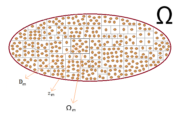
Figure 1: An example on how the obstacles are distributed in $\Omega$.

Remark 1.2.

We see that $\bigcup^{[a^{-1}]}_{m=1}\Omega_{m}\subset\Omega$. Hence $Vol(\bigcup^{[a^{-1}]}_{m=1}\Omega_{m})=\sum^{[a^{-1}]}_{m=1}\frac{[K(z_{m})+1]}{K(z_{m})+1}a\rightarrow\int_{\Omega}\frac{[K(z)+1]}{K(z)+1}dz$ as $a\rightarrow 0$. Then, as $a\rightarrow 0$, we have $\bigcup^{[a^{-1}]}_{m=1}\Omega_{m}\varsubsetneq\Omega$ if $K$ is not a function with entire values! In this case, we might not fill in fully $\Omega$. To do it, one needs, for instance, to add $\frac{1}{L}[a^{-1}]$ sub-domains, of the form $\Omega_{m}$, with an appropriate integer $L$ depending on $\Omega\setminus{\lim_{a\rightarrow 0}\bigcup^{[a^{-1}]}_{m=1}\Omega_{m}}$. To keep the presentation simple, we take $\Omega:=\lim_{a\rightarrow 0}\bigcup^{[a^{-1}]}_{m=1}\Omega_{m}$.

We prove the following result:

Theorem 1.3.

Let the small obstacles be distributed in a bounded domain $\Omega$, say of unit volume, with their number $M:=M(a):=O(a^{-1})$ and their minimum distance $d:=d(a):=a^{t}$,  $\frac{1}{3}\leq t<\frac{5}{12}$, as $a\rightarrow 0$, as described above.

1. If the obstacles are distributed as follows: $\Omega=\cup^{N}_{j=1}E_{j}$, with $N$ fixed, and each sub-domain $\Omega_{m}$ included $E_{j}$ contains $K(z_{j})+1$ obstacles having the same shape (actually the same capacitance), then we have the asymptotic expansion:

   $$U^{\infty}(\hat{x},\theta)=U_{N}^{\infty}(\hat{x},\theta)+O(a^{\frac{1}{3}-\frac{4}{5}t}),\;a\rightarrow 0,\mbox{ uniformly in terms of }\theta\mbox{ and }\hat{x}\mbox{ in }\mathbb{S}^{2},$$ (1.18)

   where $U_{N}^{\infty}(\hat{x},\theta)$ is the farfield corresponding to the scattering problem

   $$(\Delta+\kappa^{2}-K_{N}\mathbb{C}_{N})U_{N}^{t}=0\mbox{ in }\mathbb{R}^{3},$$ (1.19)

   $$U_{N}^{t}=U_{N}^{s}+e^{i\kappa x\cdot\theta},$$ (1.20)

   $$\frac{\partial U_{N}^{s}}{\partial|x|}-i\kappa U_{N}^{s}=o\left(\frac{1}{|x|}\right),|x|\rightarrow\infty,$$ (1.21)

   where $\mathbb{C}_{N}=0,\;\mbox{in }\mathbb{R}^{3}\setminus{\overline{\Omega}}$ and $\mathbb{C}_{N}=\overline{C}_{j},\;\mbox{ in }E_{j}$, $j=1,...,N$ and $\overline{C}_{j}\;a$ is the capacitance of the (same) obstacles included in $E_{j}$. Similarly $K_{N}=0,\;\mbox{in }\mathbb{R}^{3}\setminus{\overline{\Omega}}$ and $K_{N}=K(z_{j})+1,\;\mbox{ in }E_{j}$, $j=1,...,N$.

2. If the obstacles are distributed arbitrary in $\Omega$, i.e. with different capacitances, then there exists a potential $\mathbb{C}_{0}\in\cap_{p\geq 1}L^{p}(\mathbb{R}^{3})$ with support in $\Omega$ such that

   $$\lim_{a\rightarrow 0}U^{\infty}(\hat{x},\theta)=U_{0}^{\infty}(\hat{x},\theta)\mbox{ uniformly in terms of }\theta\mbox{ and }\hat{x}\mbox{ in }\mathbb{S}^{2}$$ (1.22)

   where $U_{0}^{\infty}(\hat{x},\theta)$ is the farfield corresponding to the scattering problem

   $$(\Delta+\kappa^{2}-(K+1)\mathbb{C}_{0})U_{0}^{t}=0\mbox{ in }\mathbb{R}^{3},$$ (1.23)

   $$U_{0}^{t}=U_{0}^{s}+e^{i\kappa x\cdot\theta},$$ (1.24)

   $$\frac{\partial U_{0}^{s}}{\partial|x|}-i\kappa U_{0}^{s}=o\left(\frac{1}{|x|}\right),|x|\rightarrow\infty.$$ (1.25)

3. If in addition $K\mid_{\Omega}$ is in $C^{0,\gamma}(\Omega)$, $\gamma\in(0,1]$ and the obstacles have the same capacitances , then

   $$U^{\infty}(\hat{x},\theta)=U_{0}^{\infty}(\hat{x},\theta)+O(a^{\min\{\gamma,\frac{1}{3}-\frac{4}{5}t\}})\mbox{ uniformly in terms of }\theta\mbox{ and }\hat{x}\mbox{ in }\mathbb{S}^{2}$$ (1.26)

   where $C_{0}=C$ in $\Omega$ and $C_{0}=0$ in $\mathbb{R}^{3}\setminus{\overline{\Omega}}$.

The interesting observation behind such results is the ’equivalent’ behaviour between a collection of, appropriately dense, small holes (or impenetrable obstacles) and an extended penetrable obstacle modeled by an additive potential. Such an observation goes back at least to the works by Cioranescu and Murat [5, 6] and also the reference therein. Their analysis, made for the Poisson problem, is based on homogenization via energy methods and, in particular, they assume that the obstacles are distributed periodically. More elaborated expositions on the homogenization theory applied to related problems can be found in the books [2] and [8].

In the results presented here, we do not need such periodicity and no homogenization is used. Instead, we first use integral equation methods to derive the asymptotic expansion (1), which is deduced from [3], and second we analyze the limit, as $a$ goes to zero, of the dominant term $\sum_{m=1}^{M}e^{-i\kappa\hat{x}\cdot z_{m}}Q_{m}$ when $M:=M(a):=O(a^{-1})$ recalling that $Q_{m},m=1,...,M$ solves the Foldy-Lax algebraic system (1.11). The main ingredients in this analysis are related to the invertibility properties of this last algebraic system derived in [3], see subsection 2.1 below, and the precise treatment of the summation in the formentioned dominant term. As we can see in Theorem 1.3, the equivalent term (or the strange term recalling the terminology of Cioranescu and Murat) is composed of two terms. The first one, $K+1$, models the local number of the distributed obstacles while the second one, $\mathbb{C}_{0}$, models their geometry. In the situation discussed in [5, 6], and other references, the coefficient $K$ is reduced to zero since locally they have only one obstacle and then $t=\frac{1}{3}$, see Figure 1. It happens that this coefficient can have interesting applications in the theory of acoustic materials. Indeed, perforating a given domain by a set of holes having the same shape (balls for instance) and distributed in an appropriate way following a given function $K$, see the paragraph before Remark 1.2, then the asymptotic expansion in (1.22) says that the farfield generated by such a collection is equivalent to the one corresponding to an acoustic medium having $n(x):=\sqrt{1-\frac{(K+1)\mathbb{C}_{0}}{\kappa}}$ as an index of refraction. We can also use the geometry, i.e. the coefficient $\mathbb{C}_{0}$, instead of $K$ to derive the same conclusion. The error estimates in (1.26) measures the error between the scattered fields generated by the perforated medium and the ones related to the refraction index. In other words, these estimates measure the accuracy in the design, by perforation, of acoustic materials with desired refraction index.

Let us make some additional comments on these results related to the inversion theory. Let the small scatterers model small anomalies (i.e. tumors). Saying that the collection of the scatterers is dense ($M$ is large, $a$ and $d$ are small), means that the tumor propagates and becomes an advanced one. In this case, the equivalent medium is what we could see from the measurements collected far away. If we have access to the measured farfields corresponding to the distributed obstacles described above, then the equivalent medium can be described and quantified by solving the inverse potential scattering problem $\{U_{0}^{\infty}(\hat{x},\theta),\;\theta\mbox{ and }\hat{x}\mbox{ in }\mathbb{S}^{2}\}\rightarrow(K+1)\mathbb{C}_{0}$. In this case the error estimate in (1.26) added to the stability estimate of the inverse scattering problem help to reconstruct the effective medium from these measurements. This inverse problem is quite well studied using the methods introduced in [12, 13, 14] for instance.

A result similar to (1.22) is also derived by Ramm in several of his papers, see for instance [15], where in addition to some formal arguments, he needs some extra assumptions on the distribution of the obstacles to ensure the validity of some integral formulas. The additional contribution of our work compared to his results is that we provide asymptotics expansions with explicit error estimates, as in (1.26).

So far we studied the case when $M$ is of the order $a^{-s},\;s\in[0,1]$, as $a\rightarrow 0$. We finish this introduction by claiming that, in the case when it is of the order $a^{-s},\;s>1$, the equivalent medium is the exterior impenetrable and soft obstacle $\Omega$. However, we think that its justification and the corresponding error estimates are out reach by the mathematical tools we use in this paper. In a forthcoming work, we will analyze this situation and quantify the corresponding error estimates.

The rest of the paper is devoted to the proof of Theorem 1.3. We proceed as follows. In subsection 2.1, we recall the invertibility of the algebraic system (1.11) derived from [3]. Then, in subsection 2.2, we deal with the case when the coefficient $K$ is piecewise constant and the osbtacles are locally the same, i.e. $\mathbb{C}$ is piecewise constant, by dividing $\Omega$ into $N$ regions $E_{j}$, $j=1,...,N$. In section 2.3, we apply the results of section 2.2 to the case when $N=[a^{-1}]$ and $E_{j}=\Omega_{j}$, $j=1,...,N$, and then pass to the limit $a\rightarrow 0$. In section 2.4, we deal as in section 2.2 using the H$\ddot{\mbox{o}}$lder regularity of $K$.

2 Proof of the results

2.1 Invertibility properties of the Foldy-Lax algebraic system

We can rewrite the algebraic system (1.11) as follows;

$$Y_{m}+\sum_{\begin{subarray}{c}j=1\\ j\neq m\end{subarray}}^{M}\Phi_{\kappa}(z_{m},z_{j})\bar{C}_{j}Y_{j}a = -U^{i}(z_{m},\theta),$$ (2.1)

with $Y_{m}:=\frac{Q_{m}}{C_{m}}$ and $C_{m}:=\bar{C}_{m}a$, for $m=1,\dots,M$ and $\bar{C}_{m}$ are the capacitances of $B_{m}$’s, i.e. they are independent of $a$. We set $\hat{C}:=(\bar{C}_{1},\bar{C}_{2},\dots,\bar{C}_{M})^{\top}$ and define

$$\mathbf{B}:=\left(\begin{array}[]{ccccc}-1&-\bar{C}_{2}a\Phi_{\kappa}(z_{1},z_{2})&-\bar{C}_{3}a\Phi_{\kappa}(z_{1},z_{3})&\cdots&-\bar{C}_{M}a\Phi_{\kappa}(z_{1},z_{M})\\ -\bar{C}_{1}a\Phi_{\kappa}(z_{2},z_{1})&-1&-\bar{C}_{3}a\Phi_{\kappa}(z_{2},z_{3})&\cdots&-\bar{C}_{M}a\Phi_{\kappa}(z_{2},z_{M})\\ \cdots&\cdots&\cdots&\cdots&\cdots\\ -\bar{C}_{1}a\Phi_{\kappa}(z_{M},z_{1})&-\bar{C}_{2}a\Phi_{\kappa}(z_{M},z_{2})&\cdots&-\bar{C}_{M-1}a\Phi_{\kappa}(z_{M},z_{M-1})&-1\end{array}\right),$$

$${\hat{Y}}:=\left(\begin{array}[]{cccc}Y_{1}&Y_{2}&\ldots&Y_{M}\end{array}\right)^{\top}\text{ and }\mathrm{U}^{I}:=\left(\begin{array}[]{cccc}U^{i}(z_{1})&U^{i}(z_{2})&\ldots&U^{i}(z_{M})\end{array}\right)^{\top}.\hskip 56.9055pt$$

The following lemma insures the invertibility of the algebraic system (2.1).

Lemma 2.1.

If $a<\frac{5\pi}{3}\frac{d}{\|\hat{C}\|}$ and $t:=\min\limits_{j\neq\,m,1\leq\,j,m\leq\,M}\cos(\kappa|z_{m}-z_{j}|)\geq 0$, then the matrix $\mathbf{B}$ is invertible and the solution vector $\hat{Y}$ of (2.1) satisfies the estimate

$$\sum_{m=1}^{M}|Y_{m}|^{2}\leq 4\left(1-\frac{3ta}{5\pi\,d}\|\hat{C}\|\right)^{-2}\sum_{m=1}^{M}\left|U^{i}(z_{m})\right|^{2},$$ (2.4)

and hence the estimate

$$\begin{split}\sum_{m=1}^{M}|Y_{m}|\leq 2\left(1-\frac{3ta}{5\pi\,d}\|\hat{C}\|\right)^{-1}M\max\limits_{1\leq m\leq M}\left|U^{i}(z_{m})\right|.\end{split}$$ (2.5)

The proof of this lemma can be found in [3].

2.2 Case when the obstacles are locally the same

We define a bounded function $K^{M}:\mathbb{R}^{3}\rightarrow\mathbb{R}$ as follows:

$$K^{M}(x):=K^{M}(z_{m}):=\left\{\begin{array}[]{ccc}K(z_{m})+1&\mbox{ if }&x\in\Omega_{m}\\ 0&\mbox{ if }&x\notin\Omega_{m}\mbox{ for any }m=1,\dots,[a^{-1}].\end{array}\right.$$ (2.6)

Hence each $\Omega_{m}$ contains $[K^{M}(z_{m})]$ obstacles and $K_{max}:=\sup_{z_{m}}K^{M}(z_{m})$.

Let ${C^{M}}$ be a piecewise constant function such that ${C^{M}}|_{\Omega_{m}}=\bar{C}_{m}$ for all $m=1,\dots,M$ and vanishes outside $\Omega$. We assume that there exists a finite family of $E_{j},j=,1,...,N$ such that $\Omega=\cup^{N}_{j=1}E_{j}$ and that each $E_{j}$ contains the same obstacles. Hence it is clear that ${C^{M}}$ is piecewise constant, i.e. ${C^{M}}\arrowvert_{E_{j}}=\bar{C}^{j}\,\big{(}\in\{\bar{C}_{m}\}_{m=1}^{M}\big{)}$, a constant. Let, for each $j=1,\dots,N$, $E_{j}$ contains $N_{j}$ cubes $\{\Omega^{j}_{l}\}_{l=1}^{N_{j}}\,\big{(}\subset\{\Omega_{m}\}_{m=1}^{M}\big{)}$, which contains the obstacles $\{D^{j}_{l}\}_{l=1}^{N_{j}}\,\big{(}\subset\{D_{m}\}_{m=1}^{M}\big{)}$, associated to the same reference body, i.e. ,

$$\sum_{j=1}^{N}N_{j}=M,$$ (2.7)

$$B^{j}_{l1}=B^{j}_{l2}\mbox{ for }l1,l2\in\{1,\dots,N_{j}\} \mbox{ with }\{B^{j}_{l}\}_{l=1}^{N_{j}}\subset\{B_{m}\}_{m=1}^{M}.$$ (2.8)

and $$\{\bar{C}^{j}\}_{j=1}^{N}=\{\bar{C}^{M}\}_{m=1}^{M}={}_{j=1}^{N}\{\bar{C}^{j}_{l_{j}}\}_{l_{j}=1}^{N_{j}}.$$ (2.9)

We set $\mathbf{C}:=\max\limits_{1\leq{m}\leq{M}}\bar{C}_{m}$, then we have

$$\mathbf{C} = \max\limits_{1\leq{j}\leq{N}}\max\limits_{1\leq{l}\leq{N_{j}}}\bar{C}^{j}_{l}$$ (2.10)

$$= \max\limits_{1\leq{j}\leq{N}}\bar{C}^{j}_{l_{j}}\quad\mbox{for each}\quad l_{j}\in\{1,\dots,N_{j}\}$$

$$= \max\limits_{1\leq{j}\leq{N}}\bar{C}^{j}.$$

Consider the Lippmann-Schwinger equation

$$Y(z)+\int_{\Omega}\Phi_{\kappa}(z,y)K^{M}(y){C^{M}}(y)Y(y)dy = -U^{i}(z,\theta),z\in\Omega$$ (2.11)

and define

$$V(Y)(x):=\int_{\Omega}\Phi_{\kappa}(x,y)K^{M}(y){C^{M}}(y)Y(y)dy,\qquad x\in\mathbb{R}^{3},$$ (2.12)

then we can show that $V:{L}^{2}(\Omega)\rightarrow{H}^{2}(\varOmega)$ is a bounded operator for any bounded domain $\varOmega$ in $\mathbb{R}^{3}$, see [4], and in particular there exists a positive constant $c_{0}$ such that

$$\|V(Y)\|_{H^{2}(\Omega)}\leq c_{0}\|Y\|_{L^{2}(\Omega)}.$$ (2.13)

We have also the following lemma

Lemma 2.2.

There exists one and only one solution $Y$ of the Lippmann-Schwinger equation (2.11) and it satisfies the estimate

$$\|Y\|_{L^{\infty}(\Omega)}\leq C\|U^{i}\|_{H^{2}(\Omega)} \|\nabla Y\|_{L^{\infty}(\Omega)}\leq C^{\prime}\|U^{i}\|_{H^{2}(\tilde{\Omega})},$$ and (2.14)

where $\tilde{\Omega}$ being a large bounded domain which contains $\bar{\Omega}$.

Proof.

of Lemma 2.2

The proof of the existence and uniqueness is guaranteed by the Fredholm alternative applied to $I+V:L^{2}(\Omega)\longmapsto L^{2}(\Omega)$, see [4] for instance. Let us derive the estimates in (2.14). From the invertibility of the equation (2.11) from $L^{2}(\Omega)$ to $L^{2}(\Omega)$, we deduce that $\|Y\|_{L^{2}(\Omega)}\leq c_{1}\|U^{i}\|_{L^{2}(\Omega)}$. In addition

$$\|Y\|_{H^{2}(\Omega)} \leq \|V(Y)\|_{H^{2}(\Omega)}+\|U^{i}\|_{H^{2}(\Omega)}$$ (2.15)

$$\leq c_{0}\|Y\|_{L^{2}(\Omega)}+\|U^{i}\|_{H^{2}(\Omega)}\;(\mbox{ using }(\ref{H2normofY}))$$

$$\leq C\|U^{i}\|_{H^{2}(\Omega)}(\mbox{ by the invertibility of }(\ref{fracqcfracmain-effect-int})\mbox{ in }L^{2}(\Omega)).$$

The proof of the first part ends by the Sobolev embedding $H^{2}(\Omega)\subset L^{\infty}(\Omega)$.

Let us prove the second part. From (2.11), it can be shown that $\bar{Y}$ satisfies the partial differential equation;

$$\Delta\bar{Y} = -(\kappa^{2}-K^{M}{C^{M}})\bar{Y}\quad\mbox{in}\quad\mathbb{R}^{3}$$ (2.16)

where, with an abuse of notation,

$$\bar{Y}(x):=\left\{\begin{array}[]{ccc}Y(x)&\quad\mbox{in}&\quad\Omega\\ -\int_{\Omega}\Phi_{\kappa}(x,y)K^{M}(y){C^{M}}(y)Y(y)dy-U^{i}&\quad\mbox{in}&\quad\mathbb{R}^{3}\setminus\overline{\Omega}.\\ \end{array}\right.$$ (2.19)

Let $\tilde{\Omega}$ be a large bounded domain which contains $\bar{\Omega}$, then, by the interior estimates we deduce from (2.16) that there exist a constant $c_{3}$ such that

$$\|Y\|_{W^{2,p}(\Omega)}\leq c_{4}\|Y\|_{L^{p}(\tilde{\Omega})}$$ (2.20)

where $c_{4}:=(\kappa^{2}+K_{max}\mathbf{C})$. Again from the boundedness of the operator $V$, one can obtain $\|Y\|_{L^{p}(\tilde{\Omega})}\leq c_{p}\|Y\|_{H^{2}(\tilde{\Omega})}\leq c_{p}c_{0}\|Y\|_{L^{2}({\Omega})}+c_{p}\|U^{i}\|_{H^{2}(\tilde{\Omega})}$ for $p>0$. It allows us to write (2.20) as

$$\|Y\|_{W^{2,p}(\Omega)} \leq c_{4}c_{p}c_{0}\|Y\|_{L^{2}({\Omega})}+c_{4}c_{p}\|U^{i}\|_{H^{2}(\tilde{\Omega})}$$ (2.21)

$$\leq c_{4}c_{p}c_{0}|\Omega|^{\frac{1}{2}}\|Y\|_{L^{\infty}({\Omega})}+c_{4}c_{p}\|U^{i}\|_{H^{2}(\tilde{\Omega})}$$

$$\leq c_{5}C\|U^{i}\|_{H^{2}(\tilde{\Omega})}$$

where $c_{5}:=c_{4}c_{p}\left(c_{0}|\Omega|^{\frac{1}{2}}+\frac{1}{C}\right)$. The Sobolev embeding $W^{1,p}(\Omega)\subset L^{\infty}(\Omega)$, for $p>3$, implies that

$$\|\nabla Y\|_{L^{\infty}(\Omega)}\leq\|\nabla Y\|_{W^{1,p}(\Omega)}\leq\|Y\|_{W^{2,p}(\Omega)}$$ (2.22)

for $p>3$. Hence, (2.21) and (2.22) give us the estimate

$$\|\nabla Y\|_{L^{\infty}(\Omega)}\leq C^{\prime}\|U^{i}\|_{H^{2}(\tilde{\Omega})}.$$ (2.23)

∎

Write $c_{1}:=C\|U^{i}\|_{H^{2}(\tilde{\Omega})}$, then we rewrite the estimates given in (2.14) as below

$$\|Y\|_{L^{\infty}(\Omega)}\leq c_{1} \|\nabla Y\|_{L^{\infty}(\Omega)}\leq c_{5}c_{1}.$$ and (2.24)

Observe that, for $m=1,\dots,M$, equation (2.11) can be rewritten as

$$Y(z_{m})+\sum_{\begin{subarray}{c}j=1\\ j\neq m\end{subarray}}^{M}\Phi_{\kappa}(z_{m},z_{j})\bar{C}_{j}Y(z_{j})a = -U^{i}(z_{m},\theta)$$

$$+\sum_{\begin{subarray}{c}j=1\\ j\neq m\end{subarray}}^{M}\Phi_{\kappa}(z_{m},z_{j})\bar{C}_{j}Y(z_{j})a-\sum_{\begin{subarray}{c}j=1\\ j\neq m\end{subarray}}^{[a^{-1}]}\Phi_{\kappa}(z_{m},z_{j})K^{M}(z_{j})\bar{C}_{j}Y(z_{j})Vol(\Omega_{j})$$

$$+\sum_{\begin{subarray}{c}j=1\\ j\neq m\end{subarray}}^{[a^{-1}]}\Phi_{\kappa}(z_{m},z_{j})K^{M}(z_{j})\bar{C}_{j}Y(z_{j})Vol(\Omega_{j})-\int_{\Omega}\Phi_{\kappa}(z_{m},y)K^{M}(y){C^{M}}(y)Y(y)dy.$$

We set

$$A:=\sum_{\begin{subarray}{c}j=1\\ j\neq m\end{subarray}}^{[a^{-1}]}\Phi_{\kappa}(z_{m},z_{j})K^{M}(z_{j})\bar{C}_{j}Y(z_{j})Vol(\Omega_{j})-\int_{\Omega}\Phi_{\kappa}(z_{m},y)K^{M}(y){C^{M}}(y)Y(y)dy$$

and

$$B:=\sum_{\begin{subarray}{c}j=1\\ j\neq m\end{subarray}}^{M}\Phi_{\kappa}(z_{m},z_{j})\bar{C}_{j}Y(z_{j})a-\sum_{\begin{subarray}{c}j=1\\ j\neq m\end{subarray}}^{[a^{-1}]}\Phi_{\kappa}(z_{m},z_{j})K^{M}(z_{j})\bar{C}_{j}Y(z_{j})Vol(\Omega_{j}).$$

2.2.1 Estimate of $A$

In order to evaluate this, first observe that

• $$\int_{\Omega}\Phi_{\kappa}(z_{m},y){K^{M}}(y){C^{M}}(y)Y(y)dy=\sum_{l=1}^{[a^{-1}]}\int_{\Omega_{l}}\Phi_{\kappa}(z_{m},y){K^{M}}(y){C^{M}}(y)Y(y)dy.$$ (2.26)

• For $l\neq m$, we have

  $$\int_{\Omega_{l}}\Phi_{\kappa}(z_{m},y){K^{M}}(y){C^{M}}(y)Y(y)dy-\Phi_{\kappa}(z_{m},z_{l}){K^{M}}(z_{l})\bar{C}_{l}Y(z_{l})Vol(\Omega_{l})$$

  $$=\quad{K^{M}}(z_{l})\bar{C}_{l}\int_{\Omega_{l}}\left[\Phi_{\kappa}(z_{m},y)Y(y)-\Phi_{\kappa}(z_{m},z_{l})Y(z_{l})\right]dy.$$

  Write, $f(z_{m},y)=\Phi_{\kappa}(z_{m},y)Y(y)$. Using Taylor series, we can write

  $$f(z_{m},y)-f(z_{m},z_{l})=(y-z_{l})R_{l}(z_{m},y),$$

  with

  $$R_{l}(z_{m},y) = \int_{0}^{1}\nabla_{y}f(z_{m},y-\beta(y-z_{l}))\,d\beta$$ (2.28)

  $$= \int_{0}^{1}\nabla_{y}\left[\Phi_{\kappa}(z_{m},y-\beta(y-z_{l}))Y(y-\beta(y-z_{l}))\right]\,d\beta$$

  $$= \int_{0}^{1}\left[\nabla_{y}\Phi_{\kappa}(z_{m},y-\beta(y-z_{l}))\right]Y(y-\beta(y-z_{l}))\,d\beta$$

  $$+\int_{0}^{1}\Phi_{\kappa}(z_{m},y-\beta(y-z_{l}))\left[\nabla_{y}Y(y-\beta(y-z_{l}))\right]\,d\beta.$$

  For $m=1,\dots,[a^{-1}]$ fixed, we distinguish between the cubes $\Omega_{j}$, $j\neq\,m$ which are near to $\Omega_{m}$ from the ones which are far from $\Omega_{m}$ as follows. Let $\Omega^{\prime}_{m}$, $1\leq\,m\leq\,a^{-1}$ be the balls of center $z_{m}$ and of radius $(\frac{1}{2}a^{\frac{\alpha}{3}})$ with $0<\alpha\leq 1$. The cubes lying in $\Omega^{\prime}_{m}$ will fall into the category, $N_{\Omega_{m}}$, of near by cubes and the others into the category, $F_{\Omega_{m}}$, of far cubes to $\Omega_{m}$. Since $\Omega^{\prime}_{m}$ are balls with same diameter and $\Omega_{m}$ are cubes of volume $a\frac{[K^{M}(z_{m})]}{K^{M}(z_{m})}$, the number of cubes near by $\Omega_{m}$ will not exceed $\frac{\Pi}{3}a^{\alpha-1}$ $\left[:=\frac{\frac{4}{3}\pi\left((\frac{1}{2}a^{\frac{\alpha}{3}})\right)^{3}}{a\min\limits_{m}\frac{[K^{M}(z_{m})]}{K^{M}(z_{m})}}\right]$ observing that $\frac{1}{2}\leq\frac{[K^{M}(z_{m})]}{K^{M}(z_{m})}\leq 1$.

  To make sure that at least $\Omega_{m}\subset\Omega^{\prime}_{m}$ for each $m$, we need to have ${{a}^{\frac{\alpha}{3}}\geq\sqrt{2}{a}^{\frac{1}{3}}}$. i.e. $\alpha\geq 2^{-\frac{3}{2}}$.

  Also, we have that for the cubes $\Omega_{j}\in F_{\Omega_{m}}$, we have $dist(z_{m},y)\geq\frac{1}{2}{a}^{\frac{\alpha}{3}}$ for all $y\in\Omega_{j}$ and for the cubes $\Omega_{j^{\prime}}\in N_{\Omega_{m}}\setminus\{\Omega_{m}\}$, we have $dist(z_{m},y)\geq\frac{\left(a\frac{[K^{M}(z_{m})]}{K^{M}(z_{m})}\right)^{\frac{1}{3}}}{2}\geq\frac{\left(\frac{a}{2}\right)^{\frac{1}{3}}}{2}\geq\frac{d}{2^{\frac{4}{3}}}$ for all $y\in\Omega_{j^{\prime}}$.

  From the explicit form of $\Phi_{\kappa}$, we have $\nabla_{y}\Phi_{\kappa}(x,y)=\Phi_{\kappa}(x,y)\left[\frac{1}{|x-y|}-i\kappa\right]\frac{x-y}{|x-y|},{x}\neq{y}$. Hence, we obtain that

  • for $l\neq m$ such that $\Omega_{l}\in F_{\Omega_{m}}$, we have

    $$|\Phi_{\kappa}(z_{m},y-\beta(y-z_{l}))|\leq\frac{1}{2\pi{{a}^{\frac{\alpha}{3}}}}, |\nabla_{y}\Phi_{\kappa}(z_{m},y-\beta(y-z_{l}))|\leq\frac{1}{2\pi{{a}^{\frac{\alpha}{3}}}}\left[\frac{2}{{a}^{\frac{\alpha}{3}}}+\kappa\right].$$ and

    These values give us

    $$|R_{l}(z_{m},y)| \leq \frac{1}{2\pi{{a}^{\frac{\alpha}{3}}}}\left(\left[\frac{2}{{a}^{\frac{\alpha}{3}}}+\kappa\right]\int_{0}^{1}{|Y(y-\beta(y-z_{l}))|}d\beta+\int_{0}^{1}{|\nabla_{y}Y(y-\beta(y-z_{l}))|}d\beta\right).$$

  • for $l\neq m$ such that $\Omega_{l}\in N_{\Omega_{m}}$, we have

    $$|\Phi_{\kappa}(z_{m},y-\beta(y-z_{l}))|\leq\frac{2^{\frac{1}{3}}}{2\pi{d}}, |\nabla_{y}\Phi_{\kappa}(z_{m},y-\beta(y-z_{l}))|\leq\frac{2^{\frac{1}{3}}}{2\pi{d}}\left[\frac{2^{\frac{4}{3}}}{d}+\kappa\right].$$ and

    These values give us

    $$|R_{l}(z_{m},y)| \leq \frac{2^{\frac{1}{3}}}{2\pi{d}}\left(\left[\frac{2^{\frac{4}{3}}}{d}+\kappa\right]\int_{0}^{1}{|Y(y-\beta(y-z_{l}))|}d\beta+\int_{0}^{1}{|\nabla_{y}Y(y-\beta(y-z_{l}))|}d\beta\right).$$ (2.30)

  Then, for $l\neq m$ such that $\Omega_{l}\in N_{\Omega_{m}}$, (• ‣ 2.2.1) and (2.30) imply the estimate

  $$\left|\int_{\Omega_{l}}\Phi_{\kappa}(z_{m},y){K^{M}}(y){C^{M}}(y)Y(y)dy-\Phi_{\kappa}(z_{m},z_{l}){K^{M}}(z_{l})\bar{C}_{l}Y(z_{l})Vol(\Omega_{l})\right|$$ (2.31)

  $$\leq\quad\frac{2^{\frac{1}{3}}{K^{M}}(z_{l})\bar{C}_{l}}{2\pi{d}}\left(\left[\frac{2^{\frac{4}{3}}}{d}+\kappa\right]\int_{\Omega_{l}}\left[\int_{0}^{1}{|Y(y-\beta(y-z_{l}))|}d\beta\right]|y-z_{l}|dy\right.$$

  $$\left.+\int_{\Omega_{l}}\left[\int_{0}^{1}{|\nabla_{y}Y(y-\beta(y-z_{l}))|}d\beta\right]|y-z_{l}|dy\right)$$

  $$\begin{subarray}{c}\leq\\ Lemma\ref{invertibility-of-VC}\end{subarray}\quad\frac{2^{\frac{1}{3}}{K^{M}}(z_{l})\bar{C}_{l}}{2\pi{d}}\,a^{\frac{1}{3}}\,\left(\left[\frac{2^{\frac{4}{3}}}{d}+\kappa\right]c_{1}\int_{\Omega_{l}}dy\right.\left.+|\Omega_{l}|\|\nabla{Y}\|_{L^{\infty}(\Omega_{l})}\right)$$

  $$\begin{subarray}{c}\leq\\ \eqref{interY-3}\end{subarray}\quad c_{1}2^{\frac{1}{3}}\frac{{\color[rgb]{0,0,0}[{K^{M}}(z_{l})]}\bar{C}_{l}}{2\pi{d}}\,a\,\,a^{\frac{1}{3}}\,\left(\left[\frac{2^{\frac{4}{3}}}{d}+\kappa\right]\right.\left.+c_{5}\right).$$

  In the similar way, for $l\neq m$ such that $\Omega_{l}\in F_{\Omega_{m}}$, we obtain the following estimate using (• ‣ 2.2.1) and (– ‣ • ‣ 2.2.1) ;

  $$\left|\int_{\Omega_{l}}\Phi_{\kappa}(z_{m},y){K^{M}}(y){C^{M}}(y)Y(y)dy-\Phi_{\kappa}(z_{m},z_{l}){K^{M}}(z_{l})\bar{C}_{l}Y(z_{l})Vol(\Omega_{l})\right|$$ (2.32)

  $$\leq\quad c_{1}\frac{{\color[rgb]{0,0,0}[{K^{M}}(z_{l})]}\bar{C}_{l}}{2\pi{{a}^{\frac{\alpha}{3}}}}\left(\left[\frac{2}{{a}^{\frac{\alpha}{3}}}+\kappa\right]+c_{5}\right)\,a^{\frac{1}{3}}\,a.$$

• Let us estimate the integral value $\int_{\Omega_{m}}\Phi_{\kappa}(z_{m},y){C^{M}}(y)Y(y)dy$. We have the following estimates:

  $$\left|\int_{\Omega_{m}}\Phi_{\kappa}(z_{m},y){K^{M}}(y){C^{M}}(y)Y(y)dy\right| \leq c_{1}{K^{M}}(z_{m})\bar{C}_{m}\left|\int_{\Omega_{m}}\Phi_{\kappa}(z_{m},y)dy\right|$$ (2.36)

  $$\leq \frac{1}{4\pi}c_{1}{K^{M}}(z_{m})\bar{C}_{m}\left(\int_{B(z_{m},r)}\frac{1}{|z_{m}-y|}dy+\int_{\Omega_{m}\setminus B(z_{m},r)}\frac{1}{|z_{m}-y|}dy\right)$$

  $${(\frac{1}{|z_{m}-y|}\in L^{1}(B(z_{m},r)),r<\frac{a^{\frac{1}{3}}}{2})}$$

  $$\leq \frac{1}{4\pi}c_{1}{K^{M}}(z_{m})\bar{C}_{m}\left(\sigma(\mathbb{S}^{3-1})\int_{0}^{r}\frac{1}{s}s^{3-1}ds+\frac{1}{r}Vol(\Omega_{m}\setminus B(z_{m},r))\right)$$

  $$= \frac{1}{4\pi}c_{1}{K^{M}}(z_{m})\bar{C}_{m}\underbrace{\left(2\pi r^{2}+\frac{1}{r}\left[a-\frac{4}{3}\pi r^{3}\right]\right)}_{=:lm(r,a)}$$

  $$\leq \frac{1}{4\pi}c_{1}{K^{M}}(z_{m})\mathbf{C}~{}lm(r^{c},a),$$

  $$\mbox{ $r^{c}$ is the value of $r$ where $lm(r,a)$ attains maximum}.$$

  $${\partial_{r}lm(r,a)=0\Rightarrow 4\pi r-\frac{a}{r^{2}}-\frac{8}{3}\pi r=0\Rightarrow r_{c}=\left(\frac{3}{4}\pi a\right)^{\frac{1}{3}}}$$

  $${\begin{array}[]{ccc}lm(r_{c},a)&=&2\pi\left(\frac{3}{4}\pi\right)^{\frac{2}{3}}a^{\frac{2}{3}}+\left(\frac{4}{3\pi}\right)^{\frac{1}{3}}a^{\frac{2}{3}}-\frac{4}{3}\pi\left(\frac{3}{4}\pi\right)^{\frac{2}{3}}a^{\frac{2}{3}}\\ &&\\ &=&\left[\frac{2}{3\pi}\left(\frac{3}{4}\pi\right)^{\frac{2}{3}}+\left(\frac{4}{3\pi}\right)^{\frac{1}{3}}\right]a^{\frac{2}{3}}=\frac{3}{2}\left(\frac{4}{3\pi}\right)^{\frac{1}{3}}a^{\frac{2}{3}}\end{array}}$$

  $$= \frac{3}{8\pi}c_{1}K_{max}\mathbf{C}\left(\frac{4}{3\pi}\right)^{\frac{1}{3}}a^{\frac{2}{3}}.$$ (2.37)

2.2.2 Estimate of $B$

$$\sum_{\begin{subarray}{c}j=1\\ j\neq m\end{subarray}}^{M}\Phi_{\kappa}(z_{m},z_{j})\bar{C}_{j}Y(z_{j})a-\sum_{\begin{subarray}{c}j=1\\ j\neq m\end{subarray}}^{[a^{-1}]}\Phi_{\kappa}(z_{m},z_{j})K^{M}(z_{j})\bar{C}_{j}Y(z_{j})Vol(\Omega_{j})=$$

$$\sum_{\begin{subarray}{c}l=1\\ l\neq m\\ z_{l}\in\Omega_{m}\end{subarray}}^{{\color[rgb]{0,0,0}[K^{M}(z_{m})]}}\Phi_{\kappa}(z_{m},z_{l})\bar{C}_{l}Y(z_{l})a+\sum_{\begin{subarray}{c}j=1\\ j\neq m\end{subarray}}^{[a^{-1}]}\sum_{\begin{subarray}{c}l=1\\ z_{l}\in\Omega_{j}\end{subarray}}^{{\color[rgb]{0,0,0}[K^{M}(z_{j})]}}\Phi_{\kappa}(z_{m},z_{l})\bar{C}_{l}Y(z_{l})a-\sum_{\begin{subarray}{c}j=1\\ j\neq m\end{subarray}}^{[a^{-1}]}\Phi_{\kappa}(z_{m},z_{j})K^{M}(z_{j})\bar{C}_{j}Y(z_{j})Vol(\Omega_{j})=$$

$$\bar{C}_{m}a\sum_{\begin{subarray}{c}l=1\\ l\neq m\\ z_{l}\in\Omega_{m}\end{subarray}}^{{\color[rgb]{0,0,0}[K^{M}(z_{m})]}}\Phi_{\kappa}(z_{m},z_{l})Y(z_{l})+\sum_{\begin{subarray}{c}j=1\\ j\neq m\end{subarray}}^{[a^{-1}]}\bar{C}_{j}a\big{[}\big{(}\sum_{\begin{subarray}{c}l=1\\ z_{l}\in\Omega_{j}\end{subarray}}^{{\color[rgb]{0,0,0}[K^{M}(z_{j})]}}\Phi_{\kappa}(z_{m},z_{l})Y(z_{l})\big{)}-\Phi_{\kappa}(z_{m},z_{j}){\color[rgb]{0,0,0}[K^{M}(z_{j})]}Y(z_{j})\big{]},$$

since $Vol(\Omega_{j})=a\frac{{\color[rgb]{0,0,0}[K^{M}(z_{j})]}}{K^{M}(z_{j})}\;\mbox{ and }\bar{C}_{l}=\bar{C}_{j},\mbox{ for }l=1,...,\;K^{M}(z_{j}).$ We write,

$$E^{j}_{1} := \sum_{\begin{subarray}{c}l=1\\ l\neq m\\ z_{l}\in\Omega_{m}\end{subarray}}^{{\color[rgb]{0,0,0}[K^{M}(z_{m})]}}\Phi_{\kappa}(z_{m},z_{l})Y(z_{l})$$ (2.38)

and

$$E^{j}_{2} := \big{[}\big{(}\sum_{\begin{subarray}{c}l=1\\ z_{l}\in\Omega_{j}\end{subarray}}^{{\color[rgb]{0,0,0}[K^{M}(z_{j})]}}\Phi_{\kappa}(z_{m},z_{l})Y(z_{l})\big{)}-\Phi_{\kappa}(z_{m},z_{j}){\color[rgb]{0,0,0}[K^{M}(z_{j})]}Y(z_{j})\big{]}$$ (2.39)

$$= \sum_{\begin{subarray}{c}l=1\\ z_{l}\in\Omega_{j}\end{subarray}}^{{\color[rgb]{0,0,0}[K^{M}(z_{j})]}}\big{(}\Phi_{\kappa}(z_{m},z_{l})Y(z_{l})-\Phi_{\kappa}(z_{m},z_{j})Y(z_{j})\big{)}.$$

We need to estimate $\bar{C}_{m}aE^{j}_{1}$ and $\sum_{\begin{subarray}{c}j=1\\ j\neq m\end{subarray}}^{[a^{-1}]}\bar{C}_{j}aE^{j}_{2}$.

Observe that,

$$\sum_{\begin{subarray}{c}j=1\\ j\neq m\end{subarray}}^{[a^{-1}]}\bar{C}_{j}aE^{j}_{2} = \sum_{\begin{subarray}{c}j=1\\ j\neq m\\ \Omega_{j}\in N_{\Omega_{m}}\end{subarray}}^{[a^{-1}]}\bar{C}_{j}aE^{j}_{2}+\sum_{\begin{subarray}{c}j=1\\ \\ j\neq m\\ \Omega_{j}\in F_{\Omega_{m}}\end{subarray}}^{[a^{-1}]}\bar{C}_{j}aE^{j}_{2}.$$ (2.40)

Now by writing $f^{\prime}(z_{m},y):=\Phi_{\kappa}(z_{m},y)Y(y)$. For $z_{l}\in\Omega_{j},\,j\neq m$, using Taylor series, we can write

$$f^{\prime}(z_{m},z_{j})-f^{\prime}(z_{m},z_{l})=(z_{j}-z_{l})R^{\prime}(z_{m};z_{j},z_{l}),$$

with

$$R^{\prime}(z_{m};z_{j},z_{l}) = \int_{0}^{1}\nabla_{y}f^{\prime}(z_{m},z_{j}-\beta(z_{j}-z_{l}))\,d\beta.$$ (2.41)

By doing the computations similar to the ones we have performed in (2.28-2.30) and by using Lemma 2.2, we obtain

$$\left|\sum_{\begin{subarray}{c}j=1\\ j\neq m\\ \Omega_{j}\in N_{\Omega_{m}}\end{subarray}}^{[a^{-1}]}\bar{C}_{j}aE^{j}_{2}\right| \leq \frac{c_{1}2^{\frac{1}{3}}}{6}(K_{max}-1)\mathbf{C}\frac{a^{\alpha}}{{d}}\,a^{\frac{1}{3}}\,\left(\left[\frac{2^{\frac{4}{3}}}{d}+\kappa\right]\right.\left.+c_{5}\right)$$ (2.42)

$$\left|\sum_{\begin{subarray}{c}j=1\\ j\neq m\\ \Omega_{j}\in F_{\Omega_{m}}\end{subarray}}^{[a^{-1}]}\bar{C}_{j}aE^{j}_{2}\right| \leq \frac{c_{1}}{2\pi}(K_{max}-1)\mathbf{C}\frac{(a^{-1}-1)}{{{a}^{\frac{\alpha}{3}}}}\left(\left[\frac{2}{{a}^{\frac{\alpha}{3}}}+\kappa\right]+c_{5}\right)\,a^{\frac{1}{3}}\,a.$$ (2.43)

One can easily see that,

$$|\bar{C}_{m}aE^{j}_{1}| \leq \frac{c_{1}(K_{max}-1)\mathbf{C}}{4\pi}\frac{a}{d}.$$ (2.44)

Now, substitution of (2.26) in (2.2) and using the estimates (2.31), (2.32) and (2.36) associated to $A$ and the estimates (2.42), (2.43), (2.44) associated to $B$ gives us

$$Y(z_{m})+\sum_{\begin{subarray}{c}j=1\\ j\neq m\end{subarray}}^{M}\Phi_{\kappa}(z_{m},z_{j})\bar{C}_{j}Y(z_{j})a = -U^{i}(z_{m},\theta)+O\left(\frac{3}{8\pi}c_{1}K_{max}\mathbf{C}\left(\frac{4}{3\pi}\right)^{\frac{1}{3}}a^{\frac{2}{3}}\right)$$ (2.45)

$$+O\left(\frac{c_{1}K_{max}\mathbf{C}2^{\frac{1}{3}}}{6}{a}^{\alpha}\frac{a^{\frac{1}{3}}}{d}\left[\left(\frac{2^{\frac{4}{3}}}{d}+\kappa\right)+c_{5}\right]\right).$$

$$+O\left(\frac{c_{1}K_{max}\mathbf{C}}{2\pi}(a^{-1}-1)\frac{a^{\frac{4}{3}}}{{a}^{\frac{\alpha}{3}}}\left[\left(\frac{2}{{a}^{\frac{\alpha}{3}}}+\kappa\right)+c_{5}\right]\right)$$

$$+O\left(\frac{c_{1}(K_{max}-1)\mathbf{C}}{4\pi}\frac{a}{d}\right).$$

Taking the difference between (2.1) and (2.45) produces the algebraic system

$$(Y_{m}-Y(z_{m}))+\sum_{\begin{subarray}{c}j=1\\ j\neq m\end{subarray}}^{M}\Phi_{\kappa}(z_{m},z_{j})\bar{C}_{j}(Y_{j}-Y(z_{j}))a = O\left(\frac{3}{8\pi}c_{1}K_{max}\mathbf{C}\left(\frac{4}{3\pi}\right)^{\frac{1}{3}}a^{\frac{2}{3}}\right)$$

$$+O\left(\frac{c_{1}K_{max}\mathbf{C}2^{\frac{1}{3}}}{6}{a}^{\alpha}\frac{a^{\frac{1}{3}}}{d}\left[\left(\frac{2^{\frac{4}{3}}}{d}+\kappa\right)+c_{5}\right]\right)$$

$$+O\left(\frac{c_{1}K_{max}\mathbf{C}}{2\pi}(a^{-1}-1)\frac{a^{\frac{4}{3}}}{{a}^{\frac{\alpha}{3}}}\left[\left(\frac{2}{{a}^{\frac{\alpha}{3}}}+\kappa\right)+c_{5}\right]\right)$$

$$+O\left(\frac{c_{1}(K_{max}-1)\mathbf{C}}{4\pi}\frac{a}{d}\right).$$

Comparing this system with (2.1) and by using Lemma 2.1, we obtain the estimate

$$\sum_{m=1}^{M}(Y_{m}-Y(z_{m})) = O\left(\left(M\frac{3}{8\pi}c_{1}K_{max}\mathbf{C}\left(\frac{4}{3\pi}\right)^{\frac{1}{3}}a^{\frac{2}{3}}\right)\right.$$ (2.47)

$$\left.+M\left(\frac{c_{1}K_{max}\mathbf{C}2^{\frac{1}{3}}}{6}{a}^{\alpha}\frac{a^{\frac{1}{3}}}{d}\left[\left(\frac{2^{\frac{4}{3}}}{d}+\kappa\right)+c_{5}\right]\right)\right.$$

$$\left.+M\left(\frac{c_{1}K_{max}\mathbf{C}}{2\pi}(a^{-1}-1)\frac{a^{\frac{4}{3}}}{{a}^{\frac{\alpha}{3}}}\left[\left(\frac{2}{{a}^{\frac{\alpha}{3}}}+\kappa\right)+c_{5}\right]\right)\right.$$

$$\left.+M\left(\frac{c_{1}(K_{max}-1)\mathbf{C}}{4\pi}\frac{a}{d}\right)\right).$$

For the special case $d=a^{t},\,M=O(a^{-s})$ with $t,s>0$, we have the following approximation of the far-field from the Foldy-Lax asymptotic expansion (1.10) and from the definitions $Y_{m}:=\frac{Q_{m}}{C_{m}}$ and $C_{m}:=\bar{C}_{m}a$, for $m=1,\dots,M$:

$$U^{\infty}(\hat{x},\theta) = \sum_{j=1}^{M}e^{-i\kappa\hat{x}\cdot z_{j}}\bar{C}_{j}Y_{j}a$$

$$+O\left(a^{2-s}+a^{3-s-5t+3t\alpha}+a^{4-s-9t+6t\alpha}+a^{3-2s-2t\alpha}+a^{4-3s-3t\alpha}+a^{4-2s-5t+2t\alpha}\right).$$

Consider the far-field of type:

$$U^{\infty}_{C^{M}}(\hat{x},\theta) = \int_{\Omega}e^{-i\kappa\hat{x}\cdot{y}}{K^{M}}(y){C^{M}}(y)Y(y)dy.$$ (2.49)

Taking the difference between (2.49) and (2.2.2) gives us:

$$U^{\infty}_{C^{M}}(\hat{x},\theta)-U^{\infty}(\hat{x},\theta) = \int_{\Omega}e^{-i\kappa\hat{x}\cdot{y}}{K^{M}}(y){C^{M}}(y)Y(y)dy-\sum_{j=1}^{M}e^{-i\kappa\hat{x}\cdot z_{j}}\bar{C}_{j}Y_{j}a$$

$$+O\left(a^{2-s}+a^{3-s-5t+3t\alpha}+a^{4-s-9t+6t\alpha}+a^{3-2s-2t\alpha}+a^{4-3s-3t\alpha}+a^{4-2s-5t+2t\alpha}\right)$$

$$= \sum_{j=1}^{[a^{-1}]}\int_{\Omega_{j}}e^{-i\kappa\hat{x}\cdot{y}}{K^{M}}(y){C^{M}}(y)Y(y)dy-\sum_{j=1}^{[a^{-1}]}\sum_{\begin{subarray}{c}l=1\\ z_{l}\in\Omega_{j}\end{subarray}}^{{\color[rgb]{0,0,0}[K^{M}(z_{j})]}}e^{-i\kappa\hat{x}\cdot z_{l}}\bar{C}_{l}Y_{l}a$$

$$+O\left(a^{2-s}+a^{3-s-5t+3t\alpha}+a^{4-s-9t+6t\alpha}+a^{3-2s-2t\alpha}+a^{4-3s-3t\alpha}+a^{4-2s-5t+2t\alpha}\right)$$

$$= \sum_{j=1}^{[a^{-1}]}{K^{M}}(z_{j})\bar{C}_{j}\int_{\Omega_{j}}\left[e^{-i\kappa\hat{x}\cdot{y}}Y(y)-e^{-i\kappa\hat{x}\cdot z_{j}}Y(z_{j})\right]dy$$

$$+\sum_{j=1}^{[a^{-1}]}\bar{C}_{j}a\left[\sum_{\begin{subarray}{c}l=1\\ z_{l}\in\Omega_{j}\end{subarray}}^{{\color[rgb]{0,0,0}[K^{M}(z_{j})]}}\left(e^{-i\kappa\hat{x}\cdot z_{j}}Y(z_{j})-e^{-i\kappa\hat{x}\cdot z_{l}}Y(z_{l})\right)+\sum_{\begin{subarray}{c}l=1\\ z_{l}\in\Omega_{j}\end{subarray}}^{{\color[rgb]{0,0,0}[K^{M}(z_{j})]}}e^{-i\kappa\hat{x}\cdot z_{l}}\left(Y(z_{l})-Y_{l}\right)\right]$$

$$+O\left(a^{2-s}+a^{3-s-5t+3t\alpha}+a^{4-s-9t+6t\alpha}+a^{3-2s-2t\alpha}+a^{4-3s-3t\alpha}+a^{4-2s-5t+2t\alpha}\right)$$

$$= \sum_{j=1}^{[a^{-1}]}\int_{\Omega_{j}}{K^{M}}(z_{j})\bar{C}_{j}\left[e^{-i\kappa\hat{x}\cdot{y}}Y(y)-e^{-i\kappa\hat{x}\cdot z_{j}}Y(Z_{j})\right]dy$$

$$+\sum_{j=1}^{[a^{-1}]}\bar{C}_{j}a\sum_{\begin{subarray}{c}l=1\\ z_{l}\in\Omega_{j}\end{subarray}}^{{\color[rgb]{0,0,0}[K^{M}(z_{j})]}}\left(e^{-i\kappa\hat{x}\cdot z_{j}}Y(z_{j})-e^{-i\kappa\hat{x}\cdot z_{l}}Y(z_{l})\right)+\sum_{j=1}^{M}e^{-i\kappa\hat{x}\cdot z_{j}}\bar{C}_{j}a\left[Y(z_{j})-Y_{j}\right]$$

$$+O\left(a^{2-s}+a^{3-s-5t+3t\alpha}+a^{4-s-9t+6t\alpha}+a^{3-2s-2t\alpha}+a^{4-3s-3t\alpha}+a^{4-2s-5t+2t\alpha}\right)$$

$$\begin{subarray}{c}=\\ \eqref{mazya-fnlinvert-small-ac-3-effect-dif}\end{subarray} \sum_{j=1}^{[a^{-1}]}{K^{M}}(z_{j})\bar{C}_{j}\int_{\Omega_{j}}\left[e^{-i\kappa\hat{x}\cdot{y}}Y(y)-e^{-i\kappa\hat{x}\cdot z_{j}}Y(z_{j})\right]dy$$

$$+\sum_{j=1}^{[a^{-1}]}\bar{C}_{j}a\sum_{\begin{subarray}{c}l=1\\ z_{l}\in\Omega_{j}\end{subarray}}^{{\color[rgb]{0,0,0}[K^{M}(z_{j})]}}\left(e^{-i\kappa\hat{x}\cdot z_{j}}Y(z_{j})-e^{-i\kappa\hat{x}\cdot z_{l}}Y(z_{l})\right)$$

$$\qquad+\mathbf{C}\,a\,O\left(\left(M\frac{3}{8\pi}c_{1}K_{max}\mathbf{C}\left(\frac{4}{3\pi}\right)^{\frac{1}{3}}a^{\frac{2}{3}}\right)+M\left(\frac{c_{1}(K_{max}-1)\mathbf{C}}{4\pi}\frac{a}{d}\right)\right.$$

$$\qquad\left.+M\left(\frac{c_{1}K_{max}\mathbf{C}2^{\frac{1}{3}}}{6}{a}^{\alpha}\frac{a^{\frac{1}{3}}}{d}\left[\left(\frac{2^{\frac{4}{3}}}{d}+\kappa\right)+c_{5}\right]\right)\right.$$

$$\qquad\left.+M\left(\frac{c_{1}K_{max}\mathbf{C}}{2\pi}(a^{-1}-1)\frac{a^{\frac{4}{3}}}{{a}^{\frac{\alpha}{3}}}\left[\left(\frac{2}{{a}^{\frac{\alpha}{3}}}+\kappa\right)+c_{5}\right]\right)\right)$$

$$+O\left(a^{2-s}+a^{3-s-5t+3t\alpha}+a^{4-s-9t+6t\alpha}+a^{3-2s-2t\alpha}+a^{4-3s-3t\alpha}+a^{4-2s-5t+2t\alpha}\right).$$

Now, let us estimate the difference $\sum_{j=1}^{[a^{-1}]}{K^{M}}(z_{j})\bar{C}_{j}\int_{\Omega_{j}}\left[e^{-i\kappa\hat{x}\cdot{y}}Y(y)-e^{-i\kappa\hat{x}\cdot z_{j}}Y(z_{j})\right]dy$.

• Write, $f_{1}(y)=e^{-i\kappa\hat{x}\cdot{y}}Y(y)$. Using Taylor series, we can write

  $$f_{1}(y)-f_{1}(z_{j})=(y-z_{j})R_{j}(y),$$

  with

  $$R_{j}(y) = \int_{0}^{1}\nabla_{y}f_{1}(y-\beta(y-z_{j}))\,d\beta$$ (2.51)

  $$= \int_{0}^{1}\nabla_{y}\left[e^{-i\kappa\hat{x}\cdot(y-\beta(y-z_{j}))}Y(y-\beta(y-z_{j}))\right]\,d\beta$$

  $$= \int_{0}^{1}\left[\nabla_{y}e^{-i\kappa\hat{x}\cdot(y-\beta(y-z_{j}))}\right]Y(y-\beta(y-z_{j}))\,d\beta$$

  $$+\int_{0}^{1}e^{-i\kappa\hat{x}\cdot(y-\beta(y-z_{j}))}\left[\nabla_{y}Y(y-\beta(y-z_{j}))\right]\,d\beta.$$

  We have $\nabla_{y}e^{-i\kappa\hat{x}\cdot{y}}=-i\kappa\hat{x}e^{-i\kappa\hat{x}\cdot{y}}$. It gives us

  $$|R_{j}(y)| \leq \left(\kappa\int_{0}^{1}|Y(y-\beta(y-z_{j}))|\,d\beta\,+\,\int_{0}^{1}|\nabla_{y}Y(y-\beta(y-z_{j}))|\,d\beta\right).$$ (2.52)

  Using (2.52) we get the estimate

  $$\left|\sum_{j=1}^{[a^{-1}]}{K^{M}}(z_{j})\bar{C}_{j}\int_{\Omega_{j}}\left[e^{-i\kappa\hat{x}\cdot{y}}(y)Y(y)-e^{-i\kappa\hat{x}\cdot z_{j}}Y(z_{j})\right]dy\right|$$ (2.53)

  $$\leq \sum_{j=1}^{[a^{-1}]}{K^{M}}(z_{j})\bar{C}_{j}\left(\kappa\int_{\Omega_{j}}|y-z_{j}|\int_{0}^{1}|Y(y-\beta(y-z_{j}))|\,d\beta\,dy\right)\,$$

  $$+ \,\sum_{j=1}^{[a^{-1}]}{K^{M}}(z_{j})\bar{C}_{j}\left(\int_{\Omega_{j}}|y-z_{j}|\int_{0}^{1}|\nabla_{y}Y(y-\beta(y-z_{j}))|\,d\beta\,dy\right)$$

  $$\begin{subarray}{c}\leq\\ \mbox{As in \eqref{integralonomega-subelements-abs}}\end{subarray} \sum_{j=1}^{[a^{-1}]}{K^{M}}(z_{j})\bar{C}_{j}c_{1}\,a\,a^{\frac{1}{3}}\,\left(\kappa+c_{5}\right).$$

  $$\leq K_{max}\mathbf{C}c_{1}\left(\kappa+c_{5}\right)\,a^{\frac{1}{3}}.$$

In the similar way, we can also show that,

$$\left|\sum_{j=1}^{[a^{-1}]}\bar{C}_{j}a\sum_{\begin{subarray}{c}l=1\\ z_{l}\in\Omega_{j}\end{subarray}}^{{\color[rgb]{0,0,0}[K^{M}(z_{j})]}}\left(e^{-i\kappa\hat{x}\cdot z_{j}}Y(z_{j})-e^{-i\kappa\hat{x}\cdot z_{l}}Y(z_{l})\right)\right| \leq (K_{max}-1)\mathbf{C}c_{1}\left(\kappa+c_{5}\right)\,a^{\frac{1}{3}}.$$ (2.54)

Using the estimates (2.53) and (2.54) in (2.2.2), we obatin

$$U^{\infty}_{C^{M}}(\hat{x},\theta)-U^{\infty}(\hat{x},\theta) = O\left(K_{max}a^{\frac{1}{3}}\mathbf{C}c_{1}\left(\kappa+c_{5}\right)\right)$$ (2.55)

$$+O\left(M\,a\,a^{\frac{2}{3}}\left(\frac{3}{8\pi}c_{1}K_{max}\mathbf{C}^{2}\left(\frac{4}{3\pi}\right)^{\frac{1}{3}}\right)+Ma\left(\frac{c_{1}(K_{max}-1)\mathbf{C}^{2}}{4\pi}\frac{a}{d}\right)\right.$$

$$\qquad\left.+Ma\left(\frac{c_{1}K_{max}\mathbf{C}^{2}2^{\frac{1}{3}}}{6}{a^{\alpha}}\frac{a^{\frac{1}{3}}}{d}\left[\left(\frac{2^{\frac{4}{3}}}{d}+\kappa\right)+c_{5}\right]\right)\right.$$

$$\qquad\left.+Ma\left(\frac{c_{1}K_{max}\mathbf{C}^{2}}{2\pi}(a^{-1}-1)\frac{a^{\frac{4}{3}}}{{a^{\frac{\alpha}{3}}}}\left[\left(\frac{2}{{a^{\frac{\alpha}{3}}}}+\kappa\right)+c_{5}\right]\right)\right)$$

$$+O\left(a^{2-s}+a^{3-s-5t+3t\alpha}+a^{4-s-9t+6t\alpha}+a^{3-2s-2t\alpha}+a^{4-3s-3t\alpha}+a^{4-2s-5t+2t\alpha}\right)$$

$$\begin{subarray}{c}=\\ {M=O(a^{-1})\,}\\ {d=a^{t},t<1\,}\end{subarray} O\left(a^{\frac{1}{3}}K_{max}\mathbf{C}c_{1}\left(\kappa_{\max}+c_{5}\right)\right)$$

$$+O\left(a^{\frac{2}{3}}\frac{3}{8\pi}c_{1}K_{max}\mathbf{C}^{2}\left(\frac{4}{3\pi}\right)^{\frac{1}{3}}+a^{1-t}\frac{c_{1}(K_{max}-1)\mathbf{C}^{2}}{4\pi}\right.$$

$$\qquad\left.+\frac{c_{1}K_{max}\mathbf{C}^{2}2^{\frac{1}{3}}}{6}a^{\alpha-2t}a^{\frac{1}{3}}\left[\left(2^{\frac{4}{3}}+d_{\max}\kappa_{\max}\right)+c_{5}d_{\max}\right]\right.$$

$$\qquad\left.+\frac{c_{1}K_{max}\mathbf{C}^{2}}{2\pi}\frac{a^{\frac{1-\alpha}{3}}}{2}\left[\left(2a^{-\frac{\alpha}{3}}+\kappa_{\max}\right)+c_{5}\right]\right)$$

$$+O\left(a+a^{2-5t+3t\alpha}+a^{3-9t+6t\alpha}+a^{1-2t\alpha}+a^{1-3t\alpha}+a^{2-5t+2t\alpha}\right).$$

$$= O\left(a^{\frac{1}{3}}+a^{\frac{2}{3}}+a^{1-t}+a^{\alpha-2t+\frac{1}{3}}+a^{\frac{1-2\alpha}{3}}+a^{\frac{1-\alpha}{3}}+a\right.$$

$$\qquad\left.+a^{2-5t+3t\alpha}+a^{3-9t+6t\alpha}+a^{1-2t\alpha}+a^{1-3t\alpha}+a^{2-5t+2t\alpha}\right)$$

$$= O\left(a^{1-t}+a^{\alpha-2t+\frac{1}{3}}+a^{\frac{1-2\alpha}{3}}+a^{3-9t+6t\alpha}+a^{2-5t+2t\alpha}+a^{1-3t\alpha}\right).$$

Since $Vol(\Omega)$ is of order $a^{-1}(\frac{a}{2}+\frac{d}{2})^{3}$, then we observed that ${d\leq O(a^{\frac{1}{3}}})$, otherwise this volume exploses as $a\rightarrow 0$. In particular for $d$ of the form $a^{t}$, we should have $t\geq\frac{1}{3}$. From the above we should have,

$$t\geq\frac{1}{3};\qquad 1-t>0;\qquad\alpha-2t+\frac{1}{3}>0;\qquad\frac{1-2\alpha}{3}>0;$$

$$3-9t+6t\alpha>0;\qquad 1-3t\alpha>0;\qquad 2-5t+2t\alpha>0;$$

which further reduces to

$$\frac{1}{3}\leq t<1; 0<\alpha<\frac{1}{2};\qquad t\alpha<\frac{1}{3};$$

$$2-5t+2t\alpha>0; \Longrightarrow t<\frac{2}{5-2\alpha}\,\rightarrow\,\alpha<\frac{5}{2};$$

$$1-6t+3\alpha>0; \Longrightarrow t<\frac{3\alpha+1}{6}\,\rightarrow\,{\alpha>-\frac{1}{3}};$$

$$3-9t+6t\alpha>0; \Longrightarrow t<\frac{1}{3-2\alpha}\,\rightarrow\,\alpha<\frac{3}{2}.$$

Hence for $\frac{1}{3}\leq{t}<1$, we have

$${0<\alpha<\frac{1}{2}};\qquad\frac{1-2\alpha}{3}>0;\qquad t\alpha<\frac{1}{3};\qquad 2-5t+2t\alpha>0;\qquad 1-6t+3\alpha>0;\qquad 3-9t+6t\alpha>0;$$

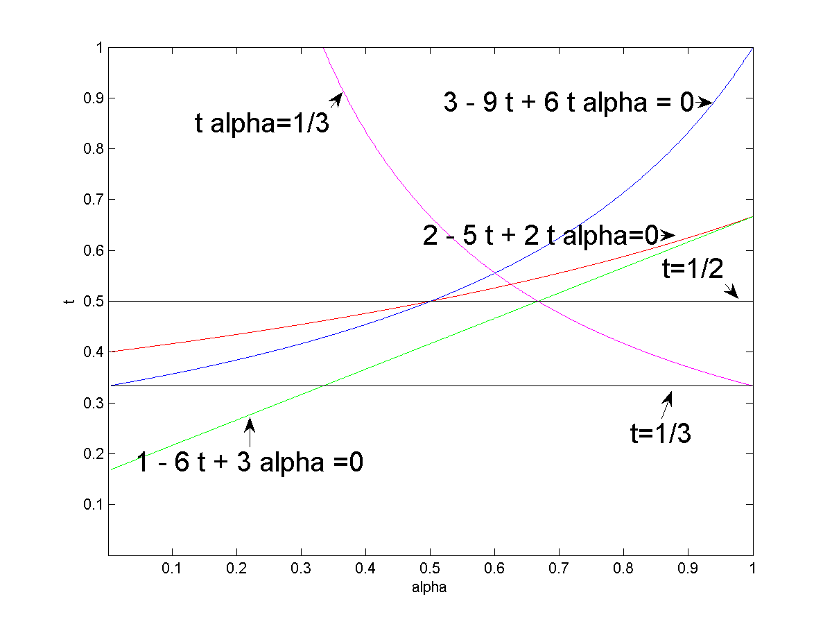
Figure 2: Relation between $\alpha$ and $t$.

By solving these inequalities, also see figure 2, we obtain $\frac{1}{3}\leq{t}<\frac{5}{12}$ and $\frac{1}{3}<{\alpha}<\frac{1}{2}$, in particular $\frac{1}{2^{\frac{3}{2}}}\leq{\alpha}<\frac{1}{2}$. Precisely,

$$U^{\infty}_{C^{M}}(\hat{x},\theta)-U^{\infty}(\hat{x},\theta) = O\left(a^{\frac{1-6t+3\alpha}{3}}+a^{\frac{1-2\alpha}{3}}\right).$$ (2.56)

Equaling the exponents in the right hand side, i.e. $\frac{1-6t+3\alpha}{3}=\frac{1-2\alpha}{3}$, we deduce that $\alpha=\frac{6}{5}t$. Hence

$$U^{\infty}_{C^{M}}(\hat{x},\theta)-U^{\infty}(\hat{x},\theta)=O\left(a^{\frac{1}{3}\left(1-\frac{12}{5}t\right)}\right).$$ (2.57)

Remark 2.3.

For the setting of each $\Omega_{m}$ containing only one obstacle $D_{m}$, $m=1,\dots,M$, i.e. $M=[a^{-1}]$ we can observe that $t=\frac{1}{3}$ and $\frac{1}{3}<\alpha<\frac{1}{2}$. In this case we can derive the estimate as

$$U^{\infty}_{C^{M}}(\hat{x},\theta)-U^{\infty}(\hat{x},\theta) = O\left(a^{\frac{3\alpha-1}{3}}+a^{\frac{1-2\alpha}{3}}\right).$$ (2.58)

It can also be written as

$$U^{\infty}_{C^{M}}(\hat{x},\theta)-U^{\infty}(\hat{x},\theta) = \left\{\begin{array}[]{ccc}O\left(a^{\frac{3\alpha-1}{3}}\right),&\mbox{ for }\frac{1}{3}<\alpha\leq\frac{2}{5},\\ {}\hfil\\ O\left(a^{\frac{1}{15}}\right),&\mbox{ for }\alpha=\frac{2}{5},\\ {}\hfil\\ O\left(a^{\frac{1-2\alpha}{3}}\right),&\mbox{ for }\frac{2}{5}\leq\alpha<\frac{1}{2}.\\ \end{array}\right.$$ (2.64)

In this case ( $s=1,t=\frac{1}{3}$ ) it is clear that the best estimate is attained for $\alpha=\frac{2}{5}$ and hence the following error estimate holds

$$U^{\infty}_{C^{M}}(\hat{x},\theta)-U^{\infty}(\hat{x},\theta) = O\left(a^{\frac{1}{15}}\right).$$ (2.65)

It can also be observed that estimate (2.56) leads to the estimate (2.65) for $t=\frac{1}{3}$.

2.3 Case when the obstacles are arbitrarily distributed

In this case, we take $N=[a^{-1}]$ and $N_{j}=1,j=1,...,N$ in the way we divide $\Omega$, i.e. $\Omega:=\cup^{[a^{-1}]}_{j=1}\Omega_{j}$, $\Omega_{j}$’s are disjoint, see the beginning of Subsection 2.2. Hence, due to the analysis in the last subsection, we end up with the following approximation

$$U^{\infty}(\hat{x},\theta)=U^{\infty}_{a}(\hat{x},\theta)+o(a^{\frac{1}{15}}),\;\;a\rightarrow 0$$ (2.66)

where $U^{\infty}_{a}(\hat{x},\theta)$ is the farfield corresponding to the following scattering problem

$$(\Delta+\kappa^{2}-K_{a}\mathbb{C}_{a})U_{a}^{t}=0\mbox{ in }\mathbb{R}^{3},$$ (2.67)

$$U_{a}^{t}=U_{a}^{s}+e^{i\kappa x\cdot\theta}$$ (2.68)

$$\frac{\partial U_{a}^{s}}{\partial|x|}-i\kappa U_{a}^{s}=o\left(\frac{1}{|x|}\right),|x|\rightarrow\infty,~{}(\text{S.R.C})$$ (2.69)

and $\mathbb{C}_{a}$ is the potential defined as follows: $\mathbb{C}_{a}=C_{j}$ in $\Omega_{j},\;j:=1,...,M$ and $\mathbb{C}_{a}=0$ in $\mathbb{R}^{3}\setminus{\overline{\Omega}}$. We have similar properties for $K_{a}$.

We know that the solution of this last scattering problem satisfies the Lippmann-Schwinger equation

$$U_{a}^{t}(x)+\int_{\Omega}K_{a}\mathbb{C}_{a}(y)\Phi(x,y)U_{a}^{t}(y)dy=e^{i\kappa x\cdot\theta},\;x\in\Omega.$$ (2.70)

In addition, we know that the function $\mathbb{C}_{a}$, defined from the sequence $(C_{j})^{M}_{j=1}$, recalling that $M=[a^{-1}]$, is bounded as function of $a\in(0,1)$ as $a\rightarrow 0$, i.e. $\mathbb{C}_{a}$ is bounded in $L^{\infty}(\Omega)$. Indeed, the capacitances of the obstacles $B_{j}$, i.e. $C_{j}$ are bounded by their Lipschitz constants, see [3], and we assumed that these Lipschitz constants are uniformly bounded. Hence $\mathbb{C}_{a}$ is bounded in $L^{2}(\Omega)$ and then there exists a function $\mathbb{C}_{0}$ in $L^{2}(\Omega)$ (actually in every $L^{p}(\Omega)$) such that $\mathbb{C}_{a}$ converges weakly to $\mathbb{C}_{0}$ in $L^{2}(\Omega)$. Now, since $K$ is continuous hence $K_{a}$ converges to $K$ in $L^{\infty}(\Omega)$ and hence in $L^{2}(\Omega)$. Then we can show that $K_{a}\mathbb{C}_{a}$ converges to $K\mathbb{C}_{0}$ in $L^{2}(\Omega)$.

Since $K\mathbb{C}_{a}$ is bounded in $L^{\infty}(\Omega)$, then from the invertibility of the Lippmann-Schwinger equation and the mapping properties of the Poisson potential, see Lemma 2.2, we deduce that $\|U_{a}^{t}\|_{H^{2}(\Omega)}$ is bounded and in particular, up to a sub-sequence, $U_{a}^{t}$ tends to $U_{0}^{t}$ in $L^{2}(\Omega)$. From the convergence of $K_{a}\mathbb{C}_{a}$ to $K\mathbb{C}_{0}$ and the one of $U_{a}^{t}$ to $U_{0}^{t}$ and (2.70), we derive the following equation satisfied by $U_{0}^{t}(x)$

$$U_{0}^{t}(x)+\int_{\Omega}K\mathbb{C}_{0}(y)\Phi(x,y)U_{0}^{t}(y)dy=e^{i\kappa x\cdot\theta}\;\mbox{ in }\Omega.$$

This is of course the Lippmann-Schwinger equation corresponding to the scattering problem

$$(\Delta+\kappa^{2}-K\mathbb{C}_{0})U_{0}^{t}=0\mbox{ in }\mathbb{R}^{3},$$ (2.71)

$$U_{0}^{t}=U_{0}^{s}+e^{i\kappa x\cdot\theta},$$ (2.72)

$$\frac{\partial U_{0}^{s}}{\partial|x|}-i\kappa U_{0}^{s}=o\left(\frac{1}{|x|}\right),|x|\rightarrow\infty,~{}(\text{S.R.C}).$$ (2.73)

As the corresponding farfields are of the form

$$U_{0}^{\infty}(\hat{x},\theta)=\int_{\Omega}e^{-i\kappa\hat{x}\cdot y}K\mathbb{C}_{0}(y)U_{0}^{t}(y)dy$$

and the ones of $U^{t}_{a}$ are of the form

$$U_{a}^{\infty}(\hat{x},\theta)=\int_{\Omega}e^{-i\kappa\hat{x}\cdot y}K_{a}\mathbb{C}_{a}(y)U_{a}^{t}(y)dy$$

we deduce that

$$U^{\infty}_{a}(\hat{x},\theta)-U^{\infty}_{0}(\hat{x},\theta)=o(1),\;a\rightarrow 0,\mbox{ uniformly in terms of }\hat{x},\theta\;\in\mathbb{S}^{2}.$$

2.4 Case when $K$ is H$\ddot{\mbox{o}}$lder continuous

Finally assume that $K\in C^{0,\gamma}(\Omega),\;\gamma\in(0,1]$, then we have the estimate $\|K-K_{a}\|_{L^{\infty}(\Omega)}\leq Ca^{\gamma}$, $a<<1$. Let $C_{0}=C$, a constant, in $\Omega$ and $C_{0}=0$ in $\mathbb{R}^{3}\setminus\Omega$. Recall that $U_{0}$ and $U_{a}$ are solutions of the Lippmann-Schwinger equations

$$U_{0}+\int_{\Omega}\Phi(x,y)K\mathbb{C}_{0}(y)U_{0}^{t}(y)dy=e^{i\kappa x\cdot\theta}$$

and

$$U_{a}+\int_{\Omega}\Phi(x,y)K_{a}\mathbb{C}_{0}(y)U_{a}^{t}(y)dy=e^{i\kappa x\cdot\theta}.$$

From the estimate $\|K-K_{a}\|_{L^{\infty}(\Omega)}\leq Ca^{\gamma}$, $a<<1$, we derive the estimate

$$U_{0}^{\infty}(\hat{x},\theta)-U^{\infty}_{a}(\hat{x},\theta)=O(a^{\gamma}),\;a<<1,\mbox{ uniformly in terms of }\hat{x},\theta\;\in\mathbb{S}^{2}.$$ (2.74)

Combining this estimate with (2.57), we deduce that

$$U^{\infty}(\hat{x},\theta)-U_{0}^{\infty}(\hat{x},\theta)=O(a^{\min{\gamma},\;\frac{1}{3}-\frac{4}{5}t}),\;a<<1,\mbox{ uniformly in terms of }\hat{x},\theta\;\in\mathbb{S}^{2}.$$ (2.75)

References

• [1] S. Albeverio, F. Gesztesy, R. Høegh-Krohn, and H. Holden. Solvable models in quantum mechanics. AMS Chelsea Publishing, Providence, RI, second edition, 2005.
• [2] A. Bensoussan; J. L. Lions and G. Papanicolaou. Asymptotic analysis for periodic structures. Studies in Mathematics and its Applications, 5. North-Holland Publishing Co., Amsterdam-New York, 1978.
• [3] D. P. Challa; M. Sini. On the justification of the Foldy-Lax approximation for the acoustic scattering by small rigid bodies of arbitrary shapes. Multiscale Model. Simul. 12 (2014), no. 1, 5508.
• [4] D. Colton and R. Kress. Inverse acoustic and electromagnetic scattering theory, volume 93 of Applied Mathematical Sciences. Springer-Verlag, Berlin, second edition, 1998.
• [5] D.  Cioranescu and F.  Murat. Un terme étrange venu d’ailleurs. (French) [A strange term brought from somewhere else] Nonlinear partial differential equations and their applications. Collège de France Seminar, Vol. II (Paris, 1979/1980), pp. 9838, 38990, Res. Notes in Math., 60, Pitman, Boston, Mass.-London, 1982.
• [6] D.  Cioranescu and F.  Murat. A strange term coming from nowhere Topics in the Mathematical Modelling of Composite Materials. Progress in Nonlinear Differential Equations and Their Applications Volume 31, 1997, pp 45-93
• [7] L. L. Foldy. The multiple scattering of waves. I. General theory of isotropic scattering by randomly distributed scatterers. Phys. Rev. (2), 67:107–119, 1945.
• [8] V. Jikov, S. Kozlov and O. Oleinik. Homogenization of differential operators and integral functionals. Springer-Verlag, 1994.
• [9] M. Lax. Multiple scattering of waves. Rev. Modern Physics, 23:287–310, 1951.
• [10] P. A. Martin. Multiple scattering, volume 107 of Encyclopedia of Mathematics and its Applications. Cambridge University Press, Cambridge, 2006. Interaction of time-harmonic waves with $N$ obstacles.
• [11] W. McLean. Strongly elliptic systems and boundary integral equations. Cambridge University Press, Cambridge, 2000.
• [12] A. I. Nachman. Reconstructions from boundary measurements. Ann. of Math. (2) 128 (1988), no. 3, 53176.
• [13] R. G. Novikov. A multidimensional inverse spectral problem for the equation $\Delta\psi+(v(x)-Eu(x))\psi=0$. Funct. Anal. Appl. 22 (1988), no. 4, 26372.
• [14] A. G. Ramm, Recovery of the potential from fixed-energy scattering data. Inverse Problems 4 (1988), no. 3, 87786.
• [15] A. G. Ramm. Many-body wave scattering by small bodies and applications. J. Math. Phys., 48(10):103511, 29, 2007.