Quantum criticality in two dimensions and Marginal Fermi Liquid

Abstract

Kinetic properties of a two dimensional model of fermions interacting with antiferromagnetic spin excitations near the quantum critical point (QCP) are considered. The temperature or doping are assumed to be sufficiently high, such that the pseudogap does not appear. In contrast to standard spin-fermion models, it is assumed that there are intrinsic inhomogeneities in the system suppressing space correlations of the antiferromagnetic excitations. It is argued that the inhomogeneities in the spin excitations in the “strange metal” phase can be a consequence of existence of “$\pi$-shifted” domain walls in the doped antiferromagnetic phase. Averaging over the inhomogeneities and calculating physical quantities like resistivity and some others one can explain unusual properties of cuprates unified under the name “Marginal Fermi Liquid” (MFL). The dependence of the slope of the linear temperature dependence of the resistivity on doping is compared with experimental data.

I Introduction

Properties of the normal state of high $T_{c}$ superconducting cuprates in the vicinity of the quantum critical point (QCP) are not consistent with the Landau Fermi liquid theory. Such unusual effects as the linear dependence of the resistivity on temperature, the linear tunnelling conductivity as a function of voltage, almost frequency and temperature independent backgrounds in the Raman-scattering intensity, constant thermal conductivity, and a very large nuclear relaxation time are similar in all $CuO$ based high-$T_{c}$ compounds. This region is usually referred to as “strange metal”.

In the pioneering work Varma et al varma1 ; abrahams0 have proposed a “marginal Fermi liquid” (MFL) phenomenology that allowed them to describe the unusual experimental findings surprisingly well. The theory is based on the assumptions that 1) electrons are scattered by unknown bosonic excitations characterized by a retarded propagator $\chi^{R}\left(\mathbf{q,}\omega,T\right),$ where $\mathbf{q}$ is momentum, $\omega$ is frequency and $T$ is temperature, 2) the imaginary part of this propagator has the form

$$\mathrm{Im}\chi^{R}\left(\mathbf{q,}\omega,T\right)=\left\{\begin{array}[]{cc}\nu\left(\omega/T\right),&\omega\ll T\\ \nu\left(sgn\omega\right),&T\ll\omega\ll\omega_{c}\end{array}\right.,$$ (1)

where $\nu$ is the density of states per unit volume and per spin direction, and $\omega_{c}$ is a high energy cutoff.

Later, Abrahams and Varma abrahams have demonstrated that the marginal Fermi liquid (MFL) assumption described results of angle-resolved photoemission (ARPES) kaminski ; valla very well, too (see, also Ref. zhu, ).

In spite of the evident success in describing the experiments gurvitch ; iye ; ando ; albenque ; cooper , the final agreement on the origin of the bosonic mode specified by Eq. (1) seems to be lacking so far. The strange metal behavior is attributed to quite different phenomena like, e.g., existence of spontaneous orbital currents varma2 , quantum criticality near antiferromagnetic transition pines ; rice ; sachdev and many others.

A recent discovery of the charge modulation in cuprates julien ; ghiringhelli ; chang ; achkar ; sebastian ; leboeuf ; blackburn ; cominSTM signals a competition between the superconductivity and a charge density wave (CDW) in the pseudogap region of the phase diagram of cuprates. Many important experimental findings of these works can be explained emp ; sachdev13a ; mepe ; hayward ; wang in the framework of the so-called spin-fermion (SF) model introduced earlier ac ; acs for description of electron-electron interaction in the vicinity of QCP. In particular, it has been proposed in Ref. emp, that the pseudogap (PG) state arises as a consequence of the competition between the superconducting and a charge modulated state.

Experimentally, increasing the temperature and doping one passes from the pseudogap state to a strange metal state described by the MFL phenomenology. Assuming that the pseudogap state can be understood in terms of the SF model it is natural to use this model also for description of the “neighboring” strange metal state. However, the correlation function of antiferromagnetic spin fluctuations used in the SF model is definitely different from the one given by Eq. (1), and new ideas are necessary to overcome this inconsistency.

In this paper we show that the MFL with the bosonic mode, Eq. (1), can nevertheless be derived from the SF model for the antiferromagnet-normal metal quantum phase transition in 2D. However, in order to achieve this goal one should introduce into the model a disorder reducing the antiferromagnetic correlations at large distances. It is argued that such a disorder is intrinsically present due to doping and, being sufficiently smooth, does not contribute to the residual resistivity.

II Formulation of the model

Following this idea we assume that the $CuO$ plains consist of domains $\mathrm{f}$, such that the antiferromagnetic (AF) field $\vec{\phi}_{\mathrm{f}}$ varies almost periodically with the modulation vector $\mathbf{Q=}\left(\pi/b,\pi/b\right)$ inside the domains but sharply changes the sign when crossing the boarder between them. In other words, the fluctuating field $\vec{\phi}_{\mathrm{f}}$ is shifted on the boarder by the lattice period $b$ (the phase of the oscillations is shifted by $\pi$) and we write it as

$$\vec{\phi}_{\mathrm{f}}\left(\mathbf{r}\right)=I_{\mathrm{f}}\left(\mathbf{r}\right)\vec{\phi}\left(\mathbf{r}\right),\quad I_{\mathrm{f}}\left(\mathbf{r}\right)=\left\{\begin{array}[]{cc}1,&\text{{f }}\in\text{{\ \textquotedblleft pink\textquotedblright}}\\ -1,&\text{{f }}\in\text{{\textquotedblleft white\textquotedblright}}\end{array}\right.,$$ (2)

In Eq. (2) the field $\vec{\phi}$ is almost periodic everywhere in space, and “pink” and “white” domains are represented in Fig. 1.

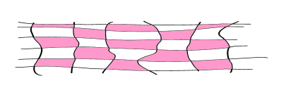
Figure 1: (Color online.) Domains separated by $\pi$-shifted domain walls.

The size and the form of the domains is not critical at the transition between the antiferromagnet and paramagnet, and Eq. (2) is assumed to be applicable on both sides of it. We write the Lagrangian $L$ of the model as

$$L=L_{0}+L_{\psi}+L_{\phi}+L_{b}$$ (3)

In Eq. (3), $L_{0}$ stands for the Lagrangian of non-interacting fermions (holes)

$$L_{0}=\int\psi^{\ast}\left(\tau,\mathbf{r}\right)\left[\partial_{\tau}+\varepsilon\left(-i\nabla_{\mathbf{r}}\right)-\mu\right]\psi\left(\tau,\mathbf{r}\right)d\mathbf{r},$$ (4)

while

$$L_{\psi\phi}=\lambda\sum_{\mathrm{f}}\int\psi^{\ast}\left(\tau,\mathbf{r}\right)\vec{\sigma}\vec{\phi}_{\mathrm{f}}\left(\tau,\mathbf{r}\right)\psi\left(\tau,\mathbf{r}\right)d\mathbf{r}$$ (5)

describes interaction of the fermions with the effective exchange field $\vec{\phi}_{\mathrm{f}}\left(\tau,\mathbf{r}\right)$ of the antiferromagnet. In Eqs. (4,5), $\psi$ is the anticommuting fermionic field, $\vec{\sigma}$ is the vector of Pauli matrices, and $\tau$ is the imaginary time. The second term in Eq. (4) stands for the electron energy operator, and $\mu$ is the chemical potential.

The Lagrangian of $L_{\phi}$ for the exchange field $\vec{\phi}$ is written near QCP as

$$L_{\phi}=\frac{1}{2}\int\Big{[}\vec{\phi}\left(\tau,\mathbf{r}\right)\left[\hat{D}_{0}^{-1}+\frac{g\vec{\phi}^{2}\left(\tau,\mathbf{r}\right)}{2}\right]\vec{\phi}\left(\tau,\mathbf{r}\right)\Big{]}d\mathbf{r},$$ (6)

where the Fourier transform of $\hat{D}_{0}$ has the form

$$D_{0}\left(\omega_{n},\mathbf{q}\right)=\left(v_{s}^{-2}\omega_{n}^{2}+\left(\mathbf{Q-q}\right)^{2}+a\right)^{-1},$$ (7)

and $\omega_{n}$ is the bosonic Matsubara frequency.

In Eq. (7), $v_{s}$ is the velocity of the spin waves, $a$ characterizes the distance from QCP ($a>0$ on the metallic side and $a<0$ in the AF region).

Actually, domain walls (DW) separating domains with opposite directions of the staggered magnetization have been found in 2D using a Hartree-Fock approximation for a $CuO$ lattice zaanen and for the $t$-$J$ model poilblanc , as well as using a mean field approximation for the Hubbard model machida . Similar DW (stripes) have been obtained later within the $t$-$J$ model numerically using the Density Matrix Renormalization Group (DMRG) method white .

The DW derived in these works separate regions with opposite direction of the AF ordering ($\pi$-shifted DW). They contain chains of holes in the middle of DW, while the magnetization vanishes there. According to this picture, the doped holes are not distributed homogeneously in the AF but are located inside the DW implying that the doped AF is intrinsically inhomogeneous. The typical distance between the DW is proportional to $p^{-1}$ zaanen ; poilblanc ; machida ; white ; tranquada , where $p$ is the number of doped holes per $Cu$ atom.

A stripe correlation of spins and holes is evident in cuprates from neutron diffraction tranquada ; kivelson . As the DW contain holes, their shape and locations are affected also by an inhomogeneous electrostatic field of doping ions located outside the $CuO$ planes. This interaction should make the shape and size of the domains rather irregular and we assume that Fig. 1 together with Eqs. (2-6) can properly describe the antiferromagnet doped with holes.

On the metallic side, $a>0$, field $\vec{\phi}$ can be finite only as a result of fluctuations. Although the AF order parameter $I_{\mathrm{f}}\vec{\phi}_{0}$ vanishes at QCP, the distance between DW determined by the hole density remains finite at $a=0$.

In the limit of a weak doping $p\sim 0.1-0.2$, the typical size of the domains $Q_{D}^{-1}\sim\left(Qp\right)^{-1}$ is considerably larger than the atomic length $Q^{-1}$, while the length $l_{T}=v_{s}/T$ can be even larger than $Q_{D}^{-1}$ for relevant temperatures.

Neglecting the quartic term in $L_{\phi},$ Eq. (6), we integrate out the field $\vec{\phi}$ and come with help of Eq. (2) to action $S_{eff}\left[\psi\right]$

$$S_{eff}\left[\psi\right]=\int_{0}^{\beta}L_{0}\left[\psi\right]d\tau+S_{int}\left[\psi\right],$$ (8)

where

$$S_{int}\left[\psi\right]=-\frac{\lambda^{2}}{2}\sum_{\mathrm{f,f}^{\prime},k=x,y,z}\int d\mathbf{r}d\mathbf{r}^{\prime}d\tau d\tau^{\prime}\psi^{\ast}\left(\tau,\mathbf{r}\right)\sigma^{k}\psi\left(\tau,\mathbf{r}\right)$$

$$\times I_{\mathrm{f}}\left(\mathbf{r}\right)I_{\mathrm{f}^{\prime}}\left(\mathbf{r}^{\prime}\right)D_{0}\left(\tau-\tau^{\prime},\mathbf{r}-\mathbf{r}^{\prime}\right)\psi^{\ast}\left(\tau^{\prime},\mathbf{r}^{\prime}\right)\sigma^{k}\psi\left(\tau^{\prime},\mathbf{r}^{\prime}\right).$$

(9)

As the DW can randomly be distorted by the potential of the $O$ atoms located outside the $CuO$ planes, averaging over random $I_{\mathrm{f}}\left(\mathbf{r}\right)$ looks a reasonable method of calculation. The propagator $D_{0}$ varies on distances of order $l_{T}$ and, in the limit $l_{T}Q_{D}\gg 1$, one can simply replace the product $I_{\mathrm{f}}I_{\mathrm{f}^{\prime}}$ in Eq. (9) by its average. We assume that the correlations are gaussian with the following moments

$$\left\langle I\left(\mathbf{r}\right)\right\rangle=0,\qquad\left\langle I\left(\mathbf{r}\right)I\left(\mathbf{r}^{\prime}\right)\right\rangle=U\left(Q_{D}\left|\mathbf{r-r}^{\prime}\right|\right),$$ (10)

where the function $U\left(x\right)$ decays sufficiently fast at $x\rightarrow\infty$ and $U\left(0\right)=1.$ Eqs. (6-10) fully specify the model considered and allow one to calculate physical quantities explicitly.

III Effective mode.

Averaging in Eq. (9) over $I\left(\mathbf{r}\right)$ we immediately come to an effective fermion-fermion interaction $\lambda^{2}\bar{D}_{0}\left(\tau-\tau^{\prime},\mathbf{r}-\mathbf{r}^{\prime}\right)$ with the propagator

$$\bar{D}_{0}\left(\tau-\tau^{\prime},\mathbf{r}-\mathbf{r}^{\prime}\right)=U\left(Q_{D}\left|\mathbf{r-r}^{\prime}\right|\right)D_{0}\left(\tau-\tau^{\prime},\mathbf{r}-\mathbf{r}^{\prime}\right).$$ (11)

Eq. (11) shows that the presence of the $\pi$-shifted DW destroys the spin correlations at distances exceeding the typical domain size $Q_{D}^{-1}$.

In the homogeneous case, the bare propagator $D_{0}$ is modified due to the Landau damping hertz . This effect can be obtained in the random phase approximation (RPA). The polarization function $\Pi\left(\omega_{n},\mathbf{q}\right)$ does not depend on $\mathbf{q}$ and is short ranged in the real space. The function $\Pi\left(\omega_{n},\mathbf{r-r}^{\prime}\right)$ is essentially non-zero only when both $\mathbf{r}$ and $\mathbf{r}^{\prime}$ are located in the same domain. Then, as in the homogeneous case, one comes to the following relation

$$D^{-1}\left(\omega_{n},\mathbf{q}\right)=D_{0}^{-1}\left(\omega_{n},\mathbf{q}\right)-\Pi\left(\omega_{n},\mathbf{q}\right),$$ (12)

where

$$\Pi\left(\omega_{n},\mathbf{q}\right)=C+\gamma\left|\omega_{n}\right|,\quad\gamma=\frac{4\lambda^{2}}{\pi v^{2}\sin\delta}$$ (13)

and $C$ is a constant renormalizing the position of the QCP. In Eq. (13), $v$ is the Fermi velocity at the hotspots and $\delta$ is the angle between the velocities of the neighboring hot spots (see, e.g., Refs.ac, ; acs, , and SI of Ref. emp, ). As usual ac ; acs ; emp , we neglect the $\omega^{2}$ -term in the propagator $D\,$, Eqs. (7, 12, 13).

Formally, the parameter $a$ entering the propagator $D\left(\omega_{n},\mathbf{q}\right)$, Eqs. (7, 12), should vanish at the transition point. However, the transition is smeared in 2D at any finite temperature by thermal fluctuations. One can estimate the characteristic width of the transition considering corrections to the coupling constant $g$ within the perturbation theory and keeping only the most divergent static contributions (SI of emp ). This gives in the first order

$$g\rightarrow g-Tg^{2}\int\frac{d^{2}k}{\left(k^{2}+a\right)^{2}},$$ (14)

which leads in the limit $a\rightarrow 0$ to a divergency. Since the transition is smeared, we conclude that $a$ cannot be effectively smaller than some minimal value $a_{0}\left(T\right)$ at which the correction in Eq. (14) is of the same order as the bare coupling $g$. This gives an estimate for $a_{0}\left(T\right)$

$$a_{0}\left(T\right)=cgT,$$ (15)

where $c$ is a numerical coefficient.

Then, one should replace parameter $a$ in Eq. (7) by

$$a\left(T\right)=a_{0}\left(T\right)+\tilde{a},$$ (16)

where $\tilde{a}$ characterizes the distance from the critical line, to obtain

$$D\left(\omega_{n},\mathbf{q}\right)=\left(\gamma\left|\omega_{n}\right|+\left(\mathbf{Q-q}\right)^{2}+a\left(T\right)\right)^{-1}$$ (17)

Replacing the function $D_{0}$ in Eq. (11) by $D$ from Eq. (17) one obtains an effective propagator $\bar{D}$ instead of $\bar{D}_{0}$

$$\bar{D}\left(\omega_{n},\mathbf{q}\right)=Q_{D}^{-2}\int\tilde{U}\left(\frac{\left|\mathbf{q-k}\right|}{Q_{D}}\right)D\left(\omega_{n},\mathbf{k}\right)\frac{d\mathbf{k}}{\left(2\pi\right)^{2}},$$ (18)

where $\tilde{U}$ is the Fourier transform of $U$.

The integration over $\mathbf{k}$ makes the propagator $\bar{D}$ weakly dependent on $\mathbf{q}$ for $\left|\mathbf{Q-q}\right|\lesssim Q_{D}.$ The analytical continuation of the propagator $D\left(\omega_{n},\mathbf{q}\right)$ from positive Matsubara frequencies $\omega_{n}$ to the real axis, $i\omega_{n}\rightarrow\omega+i0$, gives the retarded propagator $D^{R}\left(\omega,\mathbf{q},T\right)$ that can be obtained from $D\left(\omega_{n},\mathbf{q}\right)$ by the replacement $\left|\omega_{n}\right|\rightarrow i\omega$. Substituting $D^{R}\left(\omega,\mathbf{k},T\right)$ instead of $D\left(\omega_{n},\mathbf{k,}T\right)$ in Eq. (18) one can obtain the propagator $D^{R}\left(\omega,\mathbf{k,}T\right).$ The real part of $D^{R}\left(\omega,\mathbf{k,}T\right)$ is not interesting for electron transport properties. Calculation of the integral over two-dimensional momenta $\mathbf{k}$ in Eq. (18) is performed assuming that the inequality $\gamma\left|\omega\right|\lesssim Q_{D}^{2}$ is fulfilled. In this limit, the main contribution comes from $\left(\mathbf{k-Q}\right)^{2}\sim\gamma\left|\omega\right|\lesssim Q_{D}^{2}$ and the variable $\mathbf{k}$ in the function $\tilde{U}$ can be simply replaced by $\mathbf{Q}$. Then, a straightforward integration over $\mathbf{k}$ (for details, see Supplementary Information (SI)) provides

$$\mathrm{Im}\bar{D}^{R}\left(\omega,\mathbf{q},T\right)=\frac{1}{4\pi Q_{D}^{2}}\tilde{U}\left(\frac{\left|\mathbf{q-Q}\right|}{Q_{D}}\right)\arctan\left(\frac{\gamma\omega}{a\left(T\right)}\right).$$ (19)

Eq. (19) is in accord with the hypothesis of MFL, Eq. (1), for temperatures exceeding the distance from the critical line, when $a_{0}\left(T\right)\gtrsim\tilde{a}$. Provided this inequality is fulfilled, and $g$ and $\gamma$ are of the same order (as they should) one obtains the asymptotics of Eq. (1) in the limits of high $\omega\gtrsim T$ and low $\omega\lesssim T$ frequencies. The temperature $T$ should also be higher than the coupling energy between the layers, which guarantees that the spin fluctuations are effectively two-dimensional.

The function $\mathrm{Im}\bar{D}^{R}\left(\omega,\mathbf{q}\right)$, Eq. (19), is generally momentum dependent and thus differs from $\mathrm{Im}\chi^{R}\left(\mathbf{q,}\omega\right)$, Eq. (1). At the same time, the dependence of $\mathrm{Im}\bar{D}^{R}\left(\omega,\mathbf{q}\right)$, Eq. (19), is rather weak for a small size $Q_{D}^{-1}$ of the domains and the difference between the functions $\mathrm{Im}\bar{D}^{R}\left(\omega,\mathbf{q}\right)$ and $\mathrm{Im}\chi^{R}\left(\mathbf{q,}\omega\right)$ is not very important. One can see from Eq. (19) that the originally sharp dependence of the propagator $D$ on the momentum $\mathbf{Q-k}$ is smeared due to the random shapes of the domains. The function $\tilde{U}\left(\left|\mathbf{q-Q}\right|/Q_{D}\right)$ should describe a smeared shape of paramagnon peaks in neutron scattering. Experimentally observed peaks are indeed rather broad dai ; fong ; li .

The structure of the DW containing both magnetic moments and holes should result in a coupling of the mode $\bar{D}^{R}$ not only to spin but also to charge excitations.

IV Factorization of the imaginary part of self-energy into energy- and momentum-dependent parts.

Many physical quantities can be obtained using the imaginary part Im$\Sigma^{R}$ of the self-energy $\Sigma^{R}$ of the retarded one-particle electron Green function. A very important feature of the MFL hypothesis is that Im$\Sigma^{R}$ factorizes into energy-and momentum dependent parts varma1 ; abrahams0 ; abrahams . It is this property that leads finally the universal dependencies of physical quantities on temperature, energy, etc.

We calculate Im$\Sigma^{R}$ using a self-consistent Born approximation. A standard representation for Im$\Sigma^{R}\mathrm{\ }$reads

$$\mathrm{Im}\Sigma^{R}\left(\varepsilon,\mathbf{p}\right)=-\frac{\lambda^{2}}{\left(2\pi\right)^{3}}\int d\mathbf{p}_{1}\int_{-\infty}^{\infty}d\omega\mathrm{Im}G^{R}\left(\varepsilon-\omega,\mathbf{p}_{1}\right)$$

$$\times\mathrm{Im}\bar{D}^{R}\left(\omega,\mathbf{p-p}_{1}\right)\left(\tanh\frac{\varepsilon-\omega}{2T}+\coth\frac{\omega}{2T}\right),$$ (20)

where

$$G^{R}\left(\varepsilon,\mathbf{p}\right)=\left(\varepsilon-\varepsilon\left(\mathbf{p}\right)+\mu+i/\left(2\tau\left(\mathbf{p}\right)\right)\right)^{-1},$$ (21)

$$\frac{1}{2\tau\left(\mathbf{p}\right)}=\frac{1}{2\tau_{el}}-\mathrm{Im}\Sigma^{R}\left(\varepsilon,\mathbf{p}\right)$$ (22)

and $\tau_{el}$ is the elastic scattering time due to scattering on non-magnetic impurities. In principle, Eq. (20-22) is an integral equation. However, it can easily be solved assuming that the dependence of $G^{R}\left(\varepsilon,\mathbf{p}_{1}\right)$ on the component $p_{1\perp}$perpendicular to the Fermi surface is more sharp than that of $\mathrm{Im}\bar{D}^{R}\left(\omega,\mathbf{p-p}_{1}\right)$. Then, we neglect $p_{1\perp}$ in $\mathrm{Im}\bar{D}^{R}\left(\omega,\mathbf{p-p}_{1}\right)$ and integrate over this variable. The main contribution comes from the vicinity of the Fermi surface and we obtain

$$\mathrm{Im}\Sigma^{R}\left(\varepsilon,\mathbf{p}\right)=-\frac{\lambda^{2}A\left(\mathbf{p}\right)T}{\left(4\pi\right)^{2}}f\left(\frac{\varepsilon}{2T}\right),$$ (23)

where

$$A\left(\mathbf{p}\right)=Q_{D}^{-2}\int_{FS}\tilde{U}\left(\left|\mathbf{p-\mathbf{Q}-\bar{p}}_{1}\right|/Q_{D}\right)\frac{d\mathbf{\bar{p}}_{1}}{v\left(\mathbf{\bar{p}}_{1}\right)},$$ (24)

$v\left(\mathbf{\bar{p}}_{1}\right)$ is the velocity at a point $\mathbf{\bar{p}}_{1}$on the Fermi surface, the integration is performed over the Fermi surface, and

$$f\left(u\right)=\int_{-\infty}^{\infty}\left(\tanh\left(u-x\right)+\coth x\right)\arctan\left(bx\right)dx,$$ (25)

where $b=2\gamma/\left(cg\right)$ is of order $1.$The function $\mathrm{Im}\Sigma^{R}\left(\varepsilon,\mathbf{p}\right)$ is a smooth function of the position on the Fermi surface and does not depend on the elastic scattering time $\tau_{el}$.

The approximation used for the derivation of $\mathrm{Im}\Sigma^{R}\left(\varepsilon,\mathbf{p}\right)$ is applicable for $\tau^{-1}\left(\mathbf{p}\right)\ll v_{F}Q_{D}$, where $v_{F}$ is a typical Fermi velocity. For a weak scattering on impurities, one comes using Eqs. (23,24) to inequality

$$T\ll T_{1}=\left(Q_{D}v_{F}\right)^{2}/\lambda^{2}$$ (26)

At the same time, the temperature $T^{\ast}$ separating the pseudogap phase and metallic region was evaluated within the spin-fermion model in Ref. emp, as $T^{\ast}\sim 0.1\lambda^{2}$, which allows one to estimate the energy $\lambda^{2}$ as

$$\lambda^{2}\sim 2000-3000K$$ (27)

As $Q_{D}\sim pQ$, we can estimate the energy $Q_{D}v_{F}$ as

$$Q_{D}v_{F}\sim 1000K$$ (28)

Using the estimates (26, 28) one can conclude that at temperatures

$$T\lesssim 300-500K$$ (29)

the approximation used is clearly justified. Of course, the estimate does not exclude the linear temperature dependence of $\mathrm{Im}\Sigma^{R}\left(\varepsilon,\mathbf{p}\right)$ even at higher temperatures.

It is relevant to mention that the mean free path $l=v_{F}\tau$ may considerably exceed the domain size $Q_{D}^{-1}.$ Although the domain borders contain charges, the picture can be smeared due to overlap of the boarders near the quantum critical point. In addition, the charges can be screened. All this can reduce the scattering amplitudes and result in a long elastic mean free path and a rough estimation leads to a conclusion that the temperature $T_{1}$ can reach values of order $1000K$.

Remarkably, the function $\mathrm{Im}\Sigma^{R}\left(\varepsilon,\mathbf{p}\right)$, Eq. (23), factorizes into the energy- and momentum-dependent parts. Therefore, its temperature and energy dependence is the same for all parts of the Fermi surface. One can write

$$\mathrm{Im}\Sigma^{R}\left(\varepsilon,\mathbf{p}\right)\propto-\lambda^{2}\max\left(\left|\varepsilon\right|,T\right)$$ (30)

in agreement with the findings of Refs. varma1, ; abrahams0, ; abrahams, .

The electron spectral function has been compared in Ref. abrahams, with the results of the ARPES measurements of Refs. kaminski, ; valla, and a good agreement has been found. Using Eq. (19) one can describe also the other experiments discussed in Refs. varma1, ; abrahams0, ; abrahams, and, in particular, obtain linear in temperature d.c. resistivity.

V Linear temperature dependence of resistivity.

Having calculated the imaginary part Im$\Sigma^{R}\left(\varepsilon,\mathbf{p}\right)\mathrm{\ }$of the self-energy $\Sigma^{R}\left(\varepsilon,\mathbf{p}\right),$ Eqs. (24-25), we can calculate the conductivity and resistivity. The zero frequency conductivity $\sigma$ can conveniently be calculated using the Kubo-Kirkwood formula

$$\sigma=\frac{2e^{2}}{\pi}\int v_{x}^{2}\left(\mathbf{p}\right)\left[\text{{Im}}G^{R}\left(\mathbf{p}\right)\right]^{2}\frac{d\mathbf{p}}{\left(2\pi\right)^{2}},$$ (31)

where $v_{x}\left(\mathbf{p}\right)$ is the $x$-component of the velocity, $G^{R}$ is the retarded Green function taken at zero energy $\varepsilon$ and averaged over all types of disorder.

In principle, the integrand in Eq. (31) should contain the disorder average of the product of the Green functions. However, neglecting localization effects this fact is important only in the case of a smooth disorder. In the latter case one should simply replace at the end the scattering time $\tau$ by a longer transport time $\tau_{tr}$. As we consider scattering with the large vector $\mathbf{Q},$ just writing averaged Green functions can be a good approximation.

We write the Green function $G^{R}\left(\mathbf{p}\right)$ as

$$G^{R}\left(\mathbf{p}\right)=-\left[\varepsilon\left(\mathbf{p}\right)-\mu-\frac{i}{2\tau_{el}}+i\text{{Im}}\Sigma^{R}\left(\mathbf{p}\right)\right]^{-1},$$ (32)

where $\tau_{el}$ is the elastic scattering time, $\mu$ is the chemical potential and Im$\Sigma^{R}\left(\mathbf{p}\right)$ is obtained from Eq. (24-25) by putting $\varepsilon=0$. We write this function as

$$\text{{Im}}\Sigma^{R}\left(\mathbf{p}\right)=-\frac{\lambda^{2}A\left(\mathbf{p}\right)Tf\left(0\right)}{\left(4\pi\right)^{2}},$$ (33)

where the function $A\left(\mathbf{p}\right)$ and $f\left(0\right)$ are determined by Eqs. (24-25).

This allows one to express the conductivity $\sigma$ in terms of the following integral

$$\sigma=\frac{e^{2}}{\pi}\int\frac{\mathbf{v}^{2}\left(\mathbf{p}\right)}{\left[\left(\varepsilon\left(\mathbf{p}\right)-\mu\right)^{2}+\frac{1}{4\tau^{2}\left(\mathbf{p}\right)}\right]^{2}}\frac{1}{4\tau^{2}\left(\mathbf{p}\right)}\frac{d\mathbf{p}}{\left(2\pi\right)^{2}},$$ (34)

where $\tau\left(\mathbf{p}\right)$ equals

$$\frac{1}{2\tau\left(\mathbf{p}\right)}=\frac{1}{2\tau_{el}}+\frac{\lambda^{2}A\left(\mathbf{p}\right)Tf\left(0\right)}{\left(4\pi\right)^{2}}$$ (35)

As $\tau^{-1}\left(\mathbf{p}\right)$ is assumed to be not very large, such that the inequality

$$\tau^{-1}\left(\mathbf{p}\right)\ll Q_{D}v_{F}$$ (36)

is fulfilled, the main contribution into the integral (34) comes from the narrow region near the Fermi surface. This allows one to integrate separately over the perpendicular to the Fermi surface component $\mathbf{p}_{\perp}$ of the momentum using the variable $\xi=\varepsilon\left(\mathbf{p}\right)-\mu\simeq\left(\mathbf{p}_{\perp}-\mathbf{\bar{p}}\right)\mathbf{v}\left(\mathbf{\bar{p}}\right)$ and the vector on the Fermi surface $\mathbf{\bar{p}.}$

Integrating over $\xi$ we reduce the conductivity $\sigma$ to the form

$$\sigma=e^{2}\int_{FS}v\left(\mathbf{\bar{p}}\right)\tau\left(\mathbf{\bar{p}}\right)\frac{d\mathbf{\bar{p}}}{\left(2\pi\right)^{2}}\mathbf{,}$$ (37)

where $v\left(\mathbf{\bar{p}}\right)=\left|\mathbf{v}\left(\mathbf{\bar{p}}\right)\right|$ is the modulus of the velocity at the momentum $\mathbf{\bar{p}}$ on the Fermi surface and the integration in Eq. (37) is performed over the Fermi surface.

Actually, we assume that the main contribution to $\tau^{-1}\left(\mathbf{p}\right),$ Eq. (35), comes from $\mathrm{Im}\Sigma^{R}\left(\varepsilon,\mathbf{p}\right)$ and the inequality (26) is fulfilled.

Using Eq. (35) we write the resistivity $\rho$ as

$$\rho\left(T\right)=\frac{1}{e^{2}\nu_{eff}}\left[\left\langle\frac{v^{2}\left(\mathbf{\bar{p}}\right)}{2}\left(\frac{1}{2\tau_{el}}+\frac{\lambda^{2}A\left(\mathbf{\bar{p}}\right)Tf\left(0\right)}{\left(4\pi\right)^{2}}\right)^{-1}\right\rangle_{FS}\right]^{-1}$$ (38)

where the symbol $\left\langle...\right\rangle_{FS}$ stands for the average over the Fermi surface

$$\left\langle...\right\rangle_{FS}=\frac{1}{\nu_{eff}}\int_{FS}\frac{\left(...\right)}{v\left(\mathbf{\bar{p}}\right)}\frac{d\mathbf{\bar{p}}}{\left(2\pi\right)^{2}},$$ (39)

and $\nu_{eff}$ is given by the integral

$$\nu_{eff}=\frac{1}{\left(2\pi\right)^{2}}\int_{FS}\frac{d\mathbf{\bar{p}}}{v\left(\mathbf{\bar{p}}\right)}$$ (40)

The quantity $\nu_{eff}$ is the standard density of states per spin direction for a circular Fermi surface but it may numerically differ from the latter for more complex geometries.

In case of a large $Q_{D}$, when the domain size is of the same order as atomic distances or slightly exceeds the latter, the function $A\left(\mathbf{\bar{p}}\right)$ weakly depends on the momenta $\mathbf{\bar{p}}$ on the Fermi surface. This possibility is supported by the fact that there are $8$ hot spots in the Brillouin zone and the distance between them may be somewhat smaller than the antiferromagnetic vector $\mathbf{Q}$. If one neglected the dependence of $A\left(\mathbf{\bar{p}}\right)$ on $\mathbf{\bar{p}}$ one would obtain the resistivity $\rho\left(T\right)$ simply putting in Eq. (38) $A\left(\mathbf{\bar{p}}\right)=A.$ In this case, the averaging over the Fermi surface in Eq. (38) is trivial and the resistivity $\rho\left(T\right)$ takes the form

$$\rho\left(T\right)=\rho_{0}+\alpha T,$$ (41)

where $\rho_{0}$ is the residual resistivity and

$$\alpha=\frac{\lambda^{2}Af\left(0\right)}{\left(4\pi e\right)^{2}E},\quad E=\frac{1}{2}\int_{FS}v\left(\mathbf{\bar{p}}\right)\frac{d\mathbf{\bar{p}}}{\left(2\pi\right)^{2}}.$$ (42)

In Eq. (42) the parameter $E$ is an energy of the order of the Fermi energy.

The ratio of the first and second term in Eq. (41) can be arbitrary and, in particular, the $T$-dependent term can be much larger that the residual resistivity $\rho_{0}.$

As concerns the lower limit, the temperature $T$ should not be in the pseudogap region, which gives the inequality

$$T>T^{\ast}$$ (43)

In reality, at finite $\tau_{el}$ the resistivity $\rho\left(T\right)$ is not universally linear in $T$ due to a dependence of $A\left(\mathbf{\bar{p}}\right)$ on the momentum $\mathbf{\bar{p}}$ on the Fermi surface. Nevertheless, it does become linear at sufficiently high temperatures. This can be seen from the expansion in small $\left(\tau_{el}T\right)^{-1}$ of the resistivity $\rho\left(T\right)$ in Eq. (38). The calculation is straightforward and one can easily write the first three terms of the expansion of $\rho\left(T\right)$

$$\rho\left(T\right)=\left(e^{2}\nu_{eff}\right)^{-1}\left(b_{1}T+\frac{b_{0}}{\tau_{el}}+\frac{b_{-1}}{\tau_{el}^{2}T}\right),$$ (44)

$$b_{1}=\frac{\lambda^{2}f\left(0\right)}{8\pi^{2}}\left\langle\frac{v^{2}\left(\mathbf{\bar{p}}\right)}{A\left(\mathbf{\bar{p}}\right)}\right\rangle_{FS}^{-1},$$ (45)

$$b_{0}=\left\langle\frac{v^{2}\left(\mathbf{\bar{p}}\right)}{A^{2}\left(\mathbf{\bar{p}}\right)}\right\rangle_{FS}\left\langle\frac{v^{2}\left(\mathbf{\bar{p}}\right)}{A\left(\mathbf{\bar{p}}\right)}\right\rangle_{FS}^{-2},$$ (46)

$$b_{-1}=\frac{8\pi^{2}}{\lambda^{2}f\left(0\right)}\left\langle\frac{v^{2}\left(\mathbf{\bar{p}}\right)}{A\left(\mathbf{\bar{p}}\right)}\right\rangle_{FS}^{-3}$$ (47)

$$\times\Big{[}\left\langle\frac{v^{2}\left(\mathbf{\bar{p}}\right)}{A^{2}\left(\mathbf{\bar{p}}\right)}\right\rangle_{FS}^{2}-\left\langle\frac{v^{2}\left(\mathbf{\bar{p}}\right)}{A\left(\mathbf{\bar{p}}\right)}\right\rangle_{FS}\left\langle\frac{v^{2}\left(\mathbf{\bar{p}}\right)}{A^{3}\left(\mathbf{\bar{p}}\right)}\right\rangle_{FS}\Big{]}$$

It is clear from Eqs. (44-47) that the coefficient $b_{-1}$ in the third term in Eq. (44), as well as all higher terms of the expansion in $\left(\tau_{el}T\right)^{-1}$, vanishes in the case when $A\left(\mathbf{\bar{p}}\right)$ does not depend on the momentum $\mathbf{\bar{p}}$ on the Fermi surface and one comes to Eq. (41). If $A\left(\mathbf{\bar{p}}\right)$ depends on the $\mathbf{\bar{p}}$ the third term in Eq. (44) is finite but it is small in the limit $\tau_{el}T\gg 1$. The characteristic temperature $T_{1}$ of the deviation from the linear dependence depends on the form of the function $A\left(\mathbf{\bar{p}}\right)$. One can roughly estimate this temperature as

$$T_{0}=\frac{\left(4\pi\right)^{2}\left(A_{\text{{min}}}^{-1}-A_{\text{{max}}}^{-1}\right)}{2\tau_{el}\lambda^{2}f\left(0\right)},$$ (48)

where $A_{\text{{max}}}$ and $A_{\text{{min}}}$ are maximum and minimum values of $A\left(\mathbf{\bar{p}}\right)$ on the Fermi surface. One obtains the linear in $T$ behavior for temperatures $T\gtrsim T_{0}$. Of course, the inequality (43) should also be fulfilled.

Thus, using Eqs. (44, 48) we come to the conclusion that the region of the linear resistivity exists provided the following inequality is fulfilled

$$\tau_{el}^{-1}\ll\left(Q_{D}v_{F}\right)^{2}\frac{A_{\text{{max}}}A_{\text{{min}}}}{A_{\text{{max}}}-A_{\text{{min}}}}$$ (49)

Estimating typical values of $A$ as $A_{\text{{max}}}\sim\left(v_{F}Q_{D}\right)^{-1}$ and introducing a parameter $\kappa=A_{\text{{max}}}/A_{\text{{min}}}$ we rewrite the inequality (49) as

$$\tau_{el}^{-1}\ll\frac{Q_{D}v_{F}}{\kappa-1}$$ (50)

Of course, a linear temperature dependence can also be obtained in the limit $T\ll T_{0}$ when the main contribution to the resistivity comes from the scattering on impurities. However, this limit is not as interesting as the opposite limit of high temperatures.

VI Discussion and comparison with experimental data.

A model of fermions interacting with antiferromagnetic spin fluctuations has been considered. It was assumed that the interaction is random due to presence of domains with different phase of the antiferromagnetic field. As a microscopic mechanism supporting existence of these “$\pi$-shifted domains”, it was assumed that stripes are formed in the doped antiferromagnet and eventually destroy the antiferromagnetic order affecting, however, antiferromagnetic fluctuations in the metallic side. This is a new type of disorder that has not previously been considered in models of cuprates. Of course, conventional potential disorder can be present in the model as well.

Although the model is quite simple, it allows one to obtain results predicted on basis of the MFL hypothesis varma1 ; abrahams0 in a rather simple way. Of course, the model considered here is not free of assumptions and is not completely microscopical. However, it is definitely “more microscopic” than the MFL hypothesis of Refs. varma1, ; abrahams0, . It has also predictive power being able to describe the dependence of the slope of the linear temperature dependence of the resistivity on doping.

The slope $\alpha$ of the $T$-dependence does not depend on $\tau_{el}$ but the residual resistivity $\rho_{0}$ determined by $\tau_{el}$ does. This agrees with observations of Ref. albenque, . At the same time, a clear decrease of the slope with the doping has been observed in experiments ando, ; cooper, . A more detailed microscopic theory is necessary in order to describe precisely the dependence of $\alpha$ on the doping $p$ but a rough estimation can already be done using Eqs. (24, 41, 42).

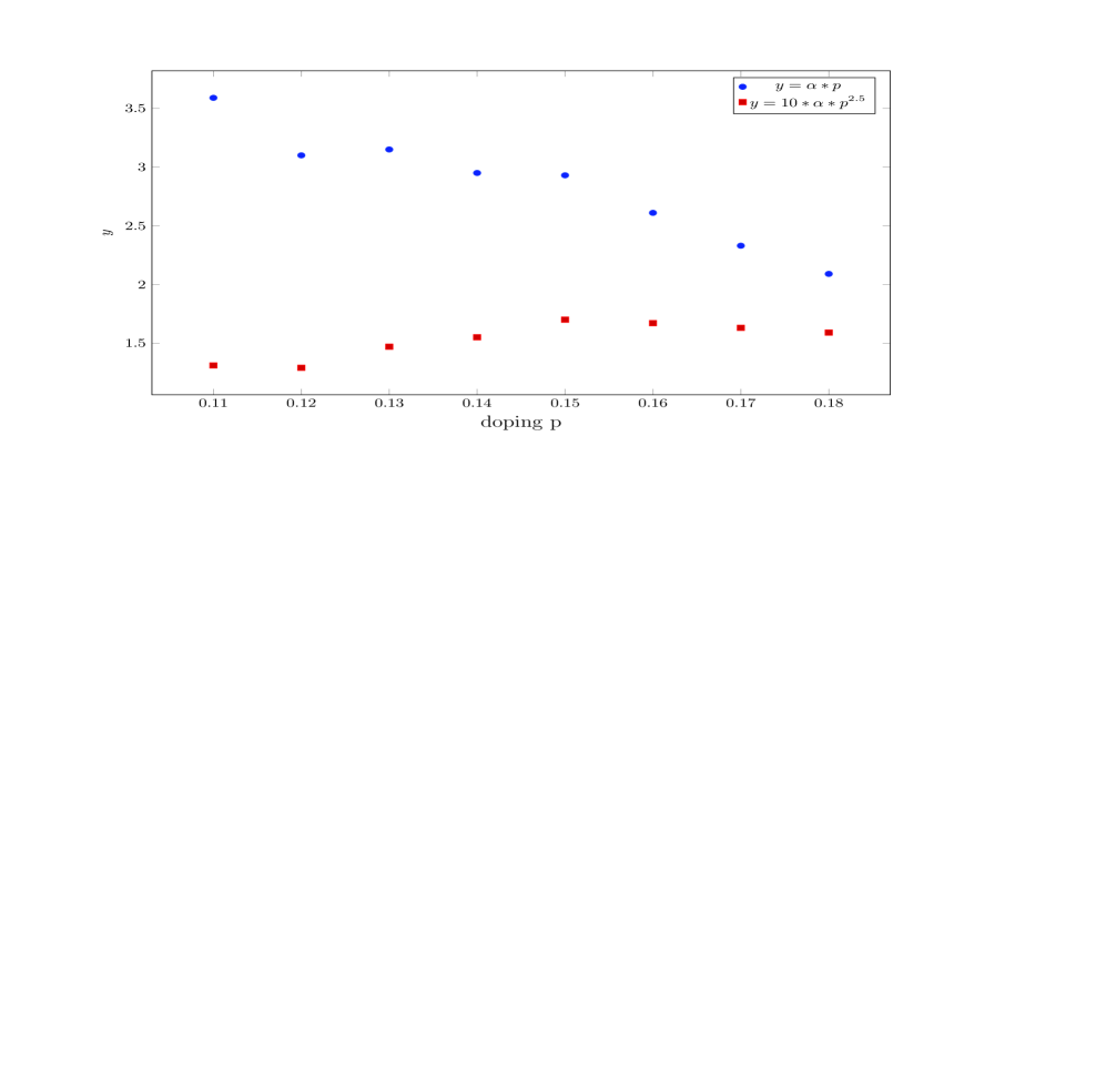
Figure 2: (Color online.) Dependence of $y=\alpha p$ (blue dots) and $y=10\alpha p^{2.5}$ (red boxes) on doping $p$ extracted from Fig.1a of Ref. ando,

We use for comparison between theory and experiment Fig.1a of Ref. ando, displaying the linear temperature dependence of resistivity Bi₂Sr_2-xLa_xCuO_6+δ for doping $p$ $=0.11-0.18$. The slope $\alpha$ is extracted from the difference $\Delta\rho=\rho\left(300K\right)-\rho\left(100K\right).$ Estimating physical quantities characterizing the fermions we simply assume that their density (volume under Fermi surface) is proportional to $pQ^{2}$ and $Q_{D}\sim pQ$ ($Q$ is inverse interatomic atomic distance). It also assumed that there are no singularities on the Fermi surface.

It is important to emphasize that the spin-fermion (SF) model contains low energy effective fermions instead of original electrons on the $CuO$ lattice. The shape of the Fermi surface of these fermions and the dependence of the Fermi energy on doping is formally not specified in the SF model and one is to be guided by reasonable assumptions. As the SF model is designed to describe the system near QCP, one has no need to think on what happens in the limit $p\rightarrow 0$ when the system becomes a Mott insulator. At the same time, in the vicinity of QCP one can reasonably assume that the density of the fermions in SF model is proportional to the density of doped electron, which leads to the proportionality of the fermion density to $pQ^{2}$. This proportionality is clearly good for comparatively high doping. As concerns low doping, it may still be a good approximation in the framework of SF model even in the antiferromagnetic region provided one stays in the vicinity of QCP.

Using the original formulation of MFL, Eq. (1), of Refs. varma1, ; abrahams0, and the fact that in SF model the density of states $\nu$ is thus independent in 2D of doping $p$ one comes to the relation $\alpha\varpropto v_{F}^{-2}\varpropto p^{-1}$. The dependence of $y=\alpha p$ on $p$ taken from Fig.1a of Ref. ando, is represented by dots in Fig. 2. Its essential dependence on $p$ indicates that Eq. (1) should possibly be modified. At the same time, it follows from Eq. (24) that $A\varpropto\left(v_{F}Q_{D}\right)^{-1}$ and $E\varpropto mv_{F}^{2}$, which leads to $\alpha\varpropto v_{F}^{-3}Q_{D}^{-1}\varpropto p^{-5/2}$. The variation of $y=10\alpha p^{5/2}$ with $p$ is represented by boxes in Fig. 2. A weak dependence of $y=\alpha p^{5/2}$ on the doping $p$ supports the present theory. As the discussion presented here is based on the assumption that the doping is not too low, it is important to emphasize that the lowest doping level $p$ studied in Ref. ando, is $p=0.11,$ which is already well in the metallic region. Therefore, the assumption that the density of states is weakly dependent on doping is not unrealistic for $p\geq 0.11$.

Anyway, the quantity $y=10\alpha p^{5/2}$ in Fig. 2 is not exactly a constant and one can speak rather of a qualitative agreement than of a microscopic theory. However, the present formulation already gives a better agreement with the experimental data than the original version of the MFL hypothesis, Eq. (1). Actually, to the best of our knowledge, the dependence of the slope on the doping is discussed here for the first time and the theory presented has a potential of further improvement.

In conclusion, fermions interacting with critical antiferromagnetic fluctuations in two dimensions are considered. Assuming that the $CuO$ planes consist of different domains, such that the coupling constant $\lambda$ changes the sign when crossing the boarders between them, we have derived the hypothetical mode of the Marginal Fermi Liquid and clarified its dependence on the doping. The slope of the linear temperature dependence of the resistivity calculated here is compared with experimental results and an encouraging agreement is found.

Appendix A Calculation of $\mathrm{Im}\bar{D}\left(\omega,\mathbf{q},T\right)$.

Here we calculate the function $\mathrm{Im}\bar{D}\left(\omega,\mathbf{q},T\right)$, where $\bar{D}^{R}\left(\omega,\mathbf{q,}T\right)$ is the analytical continuation $i\omega_{n}\rightarrow\omega+i\delta$ from Matsubara frequencies $\omega_{n}$ to real frequencies $\omega$ of the function $\bar{D}\left(\omega_{n},\mathbf{q}\right)$, Eq. (18)

$$\bar{D}\left(\omega_{n},\mathbf{q}\right)=Q_{D}^{-2}\int\tilde{U}\left(\frac{\left|\mathbf{q-k}\right|}{Q_{D}}\right)D\left(\omega_{n},\mathbf{k}\right)\frac{d\mathbf{k}}{\left(2\pi\right)^{2}},$$ (51)

with $D\left(\omega_{n},\mathbf{k}\right)$ from Eq. (17) of the main text.

$$D\left(\omega_{n},\mathbf{k}\right)=\left(\gamma\left|\omega_{n}\right|+\left(\mathbf{Q-k}\right)^{2}+a\left(T\right)\right)^{-1}.$$ (52)

The analytical continuation of propagator $D\left(\omega_{n},\mathbf{k}\right)$ can easily be performed leading to the retarded propagator

$$D^{R}\left(\omega,\mathbf{k}\right)=\left(-i\gamma\omega+\left(\mathbf{Q-k}\right)^{2}+a\left(T\right)\right)^{-1}.$$ (53)

Then, we obtain for the imaginary part of this function the following expression

$$\mathrm{Im}D^{R}\left(\omega,\mathbf{k}\right)=\frac{\gamma\omega}{\gamma^{2}\omega^{2}+\left(\left(\mathbf{Q-k}\right)^{2}+a\left(T\right)\right)^{2}}$$ (54)

Using Eq. (54) we represent $\mathrm{Im}\bar{D}\left(\omega,\mathbf{q,}T\right)$ in the form

$$\text{{Im}}\bar{D}\left(\omega,\mathbf{q,}T\right)$$

$$= Q_{D}^{-2}\int\frac{\gamma\omega\tilde{U}\left(\frac{\left|\mathbf{q-k}\right|}{Q_{D}}\right)}{\gamma^{2}\omega^{2}+\left(\left(\mathbf{Q-k}\right)^{2}+a\left(T\right)\right)^{2}}\frac{d\mathbf{k}}{\left(2\pi\right)^{2}}$$

Shifting in the integral the momentum $\mathbf{k\rightarrow k+Q}$ the function $\mathrm{Im}\bar{D}\left(\omega,\mathbf{q,}T\right)$ can be written as

$$\text{{Im}}\bar{D}\left(\omega,\mathbf{q,}T\right)$$

$$= Q_{D}^{-2}\int_{0}^{\infty}\int_{0}^{2\pi}\frac{\gamma\omega\tilde{U}\left(\frac{\sqrt{k^{2}-2k\left|\mathbf{q-Q}\right|\cos\theta+\left|\mathbf{q-Q}\right|^{2}}}{Q_{D}}\right)}{\gamma^{2}\omega^{2}+\left(k^{2}+a\left(T\right)\right)^{2}}\frac{kdkd\theta}{\left(2\pi\right)^{2}},$$

where $\theta$ is the angle between the vectors $\mathbf{k}$ and $\mathbf{q-Q}$.

In the limit $\gamma\left|\omega\right|\ll Q_{D}^{2},$ the main contribution to the integral in Eq. (A) comes from $k\sim\left(\gamma\omega\right)^{1/2}\ll Q_{D}$. This allows one to neglect $k$ in the argument of the function $\tilde{U}$. Changing the variable of the integration to $z=k^{2}$ we come to the integral

$$\text{{Im}}\bar{D}\left(\omega,\mathbf{q,}T\right)=Q_{D}^{-2}\int_{0}^{\infty}\frac{\gamma\omega\tilde{U}\left(\left|\mathbf{q-Q}\right|/Q_{D}\right)}{\gamma^{2}\omega^{2}+\left(z+a\left(T\right)\right)^{2}}\frac{dz}{4\pi},$$ (57)

Calculating the integral over $z$ we come to Eq. (19) of the main text.

Appendix B Calculation of $\mathrm{Im}\Sigma^{R}$.

A convenient representation of the imaginary part Im$\Sigma^{R}\left(\varepsilon,\mathbf{p}\right)$ can be found in Eqs. (20-22) of the main text and we use it here. Eqs. (20-22) are written in the self- consistent Born approximation. It can be obtained writing the Green functions on Matsubara frequencies and making analytical continuation to frequencies $\omega$ on the real axis. As the Green function in the integrand contains $\mathrm{Im}\Sigma^{R}\left(\varepsilon,\mathbf{p}\right)$, Eq. (20) is an integral equation and one should solve this equation in order to find this quantity. The solution is rather simple in the case when the dependence of imaginary part $\mathrm{Im}G^{R}\left(\varepsilon,\mathbf{p}_{1}\right)$ of the Green function $G^{R}$ on the component $\mathbf{p}_{1\perp}$ is more sharp than the dependence of $\mathrm{Im}\bar{D}^{R}\left(\omega,\mathbf{p-p}_{1}\right)$ on the same variable. In this situation, one may simply replace $\mathbf{p}_{1}$ in $\mathrm{Im}\bar{D}^{R}\left(\omega,\mathbf{p-p}_{1}\right)$ by its value $\mathbf{\bar{p}}_{1}$ on the Fermi surface and calculate explicitly the integral over $\mathbf{p}_{1\perp}$ in Eq. (20) using Eq. (21).

Using Eq. (21) and integrating $\mathrm{Im}G^{R}\left(\varepsilon-\omega,\mathbf{p}_{1}\right)$ over $\mathbf{p}_{1\perp}$ while keeping the parallel component of $\mathbf{p}$ fixed at a point $\mathbf{\bar{p}}_{1}$ on the Fermi surface we have

$$\int\mathrm{Im}G^{R}\left(\varepsilon-\omega,\mathbf{p}_{1}\right)d\mathbf{p}_{1\perp}=\int_{-\infty}^{\infty}\mathrm{Im}G^{R}\left(\varepsilon-\omega,\mathbf{p}_{1}\right)\frac{d\xi_{1}}{v\left(\mathbf{\bar{p}}_{1}\right)},$$ (58)

where $\xi_{1}=\varepsilon\left(\mathbf{p}_{1}\right)-\mu\simeq\mathbf{v}\left(\mathbf{\bar{p}}_{1}\right)\left(\mathbf{p}_{1}\mathbf{-\bar{p}}_{1}\right)$ and $\mathbf{v}\left(\mathbf{\bar{p}}_{1}\right)$ is the velocity on the Fermi surface at the point $\mathbf{\bar{p}}_{1}$. Neglecting the perpendicular component $\mathbf{p}_{1}-\mathbf{\bar{p}}_{1}$ in $\tau\left(\mathbf{p}_{1}\right)$ we obtain

$$\int\mathrm{Im}G^{R}\left(\varepsilon-\omega,\mathbf{p}_{1}\right)d\mathbf{p}_{1\perp}$$

$$= -\frac{1}{2\tau\left(\mathbf{\bar{p}}_{1}\right)}\int_{-\infty}^{\infty}\frac{d\xi}{\left(\varepsilon-\xi\right)^{2}+\left(2\tau\left(\mathbf{\bar{p}}_{1}\right)\right)^{-2}}=\pi$$

Substituting Eq. (B) into Eq. (20) and using Eq. (19) we come immediately to Eqs. (23-25).

References

- (1) C.M. Varma, P.B. Littlewood, S. Schmitt-Rink, E. Abrahams, A.E. Ruckenstein, Phys. Rev. Lett. 63,1996 (1989).
- (2) E. Abrahams, J. Phys. (France) 6, 2191 (1996)
- (3) E. Abrahams and C.M. Varma, Proc. Natl. Acad. Sci. 97, 5714 (2000).
- (4) A. Kaminski, J. Mesot, H. Fretwell, J. C. Campuzano, M. R. Norman, M. Randeria, H. Ding, T. Sato, T. Takahashi, T. Mochiku, K. Kadowaki, and H. Hoechst, Phys. Rev.Lett. 84, 1788 (2000).
- (5) T. Valla, A. V. Fedorov, P. D. Johnson, Q. Li, G. D. Gu, and N. Koshizuka, Phys. Rev. Lett. 85, 828 (2000).
- (6) L. Zhu, V. Aji, A. Shekhter, C.M. Varma, Phys. Rev. Lett. 100, 057001 (2008).
- (7) M. Gurvitch and A.T. Fiory, Phys. Rev. Lett. 59, 1337 (1987).
- (8) Iye Y., in “Physical Properties of High Temperature superconductors II”, D.M. Ginsberg Ed. (World Scientific, Singapore 1992).
- (9) Y. Ando, S.Komiya,K. Segawa, S. Ono,Y. Kurita, Phys. Rev. Lett. 93, 267001 (2004).
- (10) F. Rullier-Albenque et al, Eur. Lett. 81, 37008 (2008).
- (11) R. A. Cooper, Y. Wang, B. Vignolle, O. J. Lipscombe, S. M. Hayden, Y. Tanabe, T. Adachi, Y. Koike, M. Nohara, H. Takagi, Cyril Proust, and N. E. Hussey Science, 323, 603 (2009).
- (12) V. Aji and C.M. Varma, Phys. Rev. Lett. 99, 067003 (2007).
- (13) P. Monthaux and D. Pines, Phys. Rev. B 49, 4261 (1994)
- (14) R. Hlubina and T.M. Rice, Phys. Rev. B 51, 9253 (1995)
- (15) S. Sachdev, B. Keimer, Physics Today 64, 29 (2011)
- (16) T. Wu, H. Mayaffre, S. Krämer, M. Horvatić, C. Berthier, W. N. Hardy, R. Liang, D. A. Bonn, and M.-H. Julien, Nature 477, 191 (2011).
- (17) G. Ghiringhelli, M. Le Tacon, M. Minola, S. Blanco-Canosa, C. Mazzoli, N. B. Brookes, G. M. De Luca, A. Frano, D. G. Hawthorn, F. He, T. Loew, M. Moretti Sala, D. C. Peets, M. Salluzzo, E. Schierle, R. Sutarto, G. A. Sawatzky, E. Weschke, B. Keimer, and L. Braicovich, Science 337, 821 (2012).
- (18) J. Chang, E. Blackburn, A. T. Holmes, N. B. Christensen, J. Larsen, J. Mesot, Ruixing Liang, D. A. Bonn, W. N. Hardy, A. Watenphul, M. v. Zimmermann, E. M. Forgan, and S. M. Hayden, Nat. Phys. 8, 871 (2012).
- (19) A. J. Achkar, R. Sutarto, X. Mao, F. He, A. Frano, S. Blanco-Canosa, M. Le Tacon, G. Ghiringhelli, L. Braicovich, M. Minola, M. Moretti Sala, C. Mazzoli, Ruixing Liang, D. A. Bonn, W. N. Hardy, B. Keimer, G. A. Sawatzky, and D. G. Hawthorn, Phys. Rev. Lett. 109, 167001 (2012).
- (20) S.F. Sebastian, N. Harrison, and G. Lonzarich, Rep. Prog. Phys. 75, 102501 (2012).
- (21) D. LeBoeuf, S. Krämer, W. N. Hardy, R. Liang, D. A. Bonn, and Cyril Proust, Nat. Phys. 9, 79 (2013).
- (22) E. Blackburn, J. Chang, M. Hücker, A. T. Holmes, N. B. Christensen, Ruixing Liang, D. A. Bonn, W. N. Hardy, U. Rütt, O. Gutowski, M. v. Zimmermann, E. M. Forgan, and S. M. Hayden, Phys. Rev. Lett. 110, 137004 (2013).
- (23) R. Comin, A. Frano, M. M. Yee, Y. Yoshida, H. Eisaki, E. Schierle, E. Weschke, R. Sutarto, F. He, A. Soumyanarayanan, Yang He, M. Le Tacon, I. S. Elfimov, Jennifer E. Hoffman, G. A. Sawatzky, B. Keimer, A. Damascelli, Science, 343, 390 (2013).
- (24) K.B. Efetov, H. Meier, and C. Pepin, Nat. Phys. 9, 442 (2013).
- (25) S. Sachdev, R. La Placa, Phys. Rev. Lett. 111, 027202 (2013).
- (26) H. Meier, M. Einenkel, C. Pepin, K.B. Efetov, Phys. Rev. B 88, 020506(R) (2013).
- (27) L. E. Hayward, D. G. Hawthorn, R. G. Melko, S. Sachdev, Science 343, 1336 (2014).
- (28) Y. Wang, A.V. Chubukov, Phys. Rev. B 90, 035149 (2014)
- (29) Ar. Abanov, A.V. Chubukov, Phys. Rev. Lett. 84, 5608 (2000).
- (30) Ar. Abanov, A.V. Chubukov, J. Schmalian, Adv. Phys. 52, 119 (2003).
- (31) J. Zaanen and O. Gunnarsson, Phys. Rev. B 40, 7391 (1989).
- (32) K. Machida, Physica C 158, 192 (1989).
- (33) D. Poilblanc and T.M. Rice, Phys. Rev. B 39, 9749 (1989).
- (34) S. R. White and D. J. Scalapino, Phys. Rev. Lett. 80, 1272 (1998).
- (35) J. M. Tranquada, B. J. Sternlieb, J. D. Axe, Y. Nakamura, S. Uchida, Nature 375, 561 (1995).
- (36) S. A. Kivelson, I. P. Bindloss, E. Fradkin, V. Oganesyan, J. M. Tranquada, A. Kapitulnik, and C. Howald Rev. Mod. Phys. 75, 1201 (2003).
- (37) J.A. Hertz, Phys.Rev. B 14, 1165-1184 (1976).
- (38) P. Dai, H.A. Mook, R.D. Hunt, F. Dogan, Phys. Rev. B 63, 054525 (2001).
- (39) H. F. Fong, P. Bourges, Y. Sidis, L.P. Regnault, A. Ivanov, G. D. Gu, N. Koshizuka, and B. Keimer, Nature 398, 588 (1999).
- (40) Y. Li, V. Balédent, G. Yu, N. Barišić, K. Hradil, R. A. Mole, Y. Sidis, P. Steffens, X. Zhao, P. Bourges, and M. Greven, Nature 468, 283 (2010).