Autocorrelation study of the $\Theta$ transition for a coarse-grained polymer model

Abstract

By means of Metropolis Monte Carlo simulations of a coarse-grained model for flexible polymers, we investigate how the integrated autocorrelation times of different energetic and structural quantities depend on the temperature. We show that, due to critical slowing down, an extremal autocorrelation time can also be considered as an indicator for the collapse transition that helps to locate the transition point. This is particularly useful for finite systems, where response quantities such as the specific heat do not necessarily exhibit clear indications for pronounced thermal activity.

I INTRODUCTION

The necessity for a better understanding of general physical principles and mechanisms of structural transitions of polymers, such as folding, crystallization, aggregation, and the adsorption at solid and soft substrates has provoked numerous computational studies of polymer models. Autocorrelation properties of such models govern the statistical accuracy of estimated expectation values of physical quantities but also help illustrate the dynamic behavior or the relaxation properties. Verdier and co-workers were among the first to investigate autocorrelations of a simple lattice polymer approach, in which the Brownian motion of the monomers is simulated by kinetic displacements of single monomers Verdier1962 ; Verdier1966 ; Verdier1972 ; Verdier1973 . By using Monte Carlo methods, the autocorrelation functions and relaxation times of structural quantities were calculated in order to study dynamic properties of random-coil polymer chains such as the relaxation of asphericity in lattice- model chains with and without excluded volume interaction Kranbuehl1973 ; Kranbuehl1977 . More recently, these studies were extended to continuous models, where autocorrelation properties of the center-of-mass velocity, Rouse coordinates, end-to-end distance, end-to-end vector, normal modes, and the radius of gyration for polymer melts McCormick2005 ; Pestryaev2011 ; Aoyagi2001 , and of dynamic quantities of a polymer immersed in a solution Malevanets2000 ; Polson2006 ; Bishop1979 ; Rapaport1979 ; Bruns1981 ; Bansal1981 ; Mussawisade2005 were investigated. Integrated autocorrelation times are also employed to judge the efficiency of importance-sampling algorithms Nidras1997 . However, much less is known about how autocorrelation times and structural transitions of polymers depend on each other.

In the past, most of the studies on analyzing the properties of the autocorrelation times focused on spin models. The second-order phase transition between ferromagnetism and paramagnetism is characterized by a divergent spatial correlation length $\xi$ at the transition point $T_{c}$. In the thermodynamic limit (i.e., infinite system size), the divergent behavior is given by $\xi\sim\epsilon^{-\nu}$, where $\epsilon\equiv|1-T/T_{c}|$ and $\nu$ is a critical exponent Landau2000 ; NewmanMC1999 ; WJanke2002 . If an importance sampling Monte Carlo method is employed Landau2000 ; WJanke1996 ; WJanke1998 , the number of configurational updates that is needed to decorrelate the information about the history of macroscopic system states is measured by the autocorrelation time $\tau$. It is described by the power law $\tau\propto\xi^{z}\propto\epsilon^{-\nu z}$, where $z$ denotes the dynamic critical exponent, which depends on the employed algorithm Landau2000 ; NewmanMC1999 ; WJanke2002 . However, in a system of finite size, the correlation length can never really diverge. This is because the largest possible cluster has the volume $L^{d}$, where $L$ is the system size and $d$ is the dimensionality. Thus, the divergence of the correlation length as well as the autocorrelation time are “cut off” at the boundary, i.e., $\xi\lesssim L$. Consequently, $\tau\sim L^{z}$ at temperatures sufficiently close to the critical point Landau2000 ; NewmanMC1999 ; WJanke2002 . For local updates, such as single spin flips, and by using the Metropolis algorithm MetroRosTell1953 , the autocorrelation time becomes very large near the critical temperature because the dynamic critical exponent is in this case $z\approx 2$. This effect is usually called critical slowing down, but it can be reduced significantly if non-local updates, such as in Swendsen-Wang, Wolff, and multigrid algorithms NewmanMC1999 ; WJanke1998 ; Sokal1989 ; Sokal1992 , are employed. Metropolis simulations with local updates yield for the Ising model $z\approx 2.1665$ in 2D and $z\approx 2.02$ in 3D NewmanMC1999 ; Nightingale1996 ; Matz1994 . For non-local updates, numerical estimates yield a $z$ value less than unity Coddington1992 ; NewmanMC1999 ; Kandel1988 ; Kandel1989 .

Since most phase transitions in nature are of first order Gunton1983 ; Binder1987 ; Herrmann1992 ; JankeFirst-Order1994 , it is also useful to discuss autocorrelation properties near first-order phase transitions. In a finite system, the characteristic feature of a first-order transition is the double-peaked energy distribution with an entropic suppression regime between the two peaks. The dip is caused by the entropic contribution to the Boltzmann factor $\propto\text{exp}(-2\sigma L^{d-1})$, where $\sigma$ is the (reduced) interface tension and $L^{d-1}$ is the projected area of the interfaces. Thus, the dynamics in a canonical ensemble will suffer from the “supercritical slowing down”, in which the tremendous average residence time the system spends in a pure phase is described by the autocorrelation time $\tau\propto\text{exp}(2\sigma L^{d-1})$ WJanke2002 ; JankePhaseTransitions . Since this slowing down is related to the shape of the energetic probability distribution itself, it is impossible to reduce the autocorrelation time by using cluster or multigrid algorithms. The simulation in a generalized ensemble, such as multicanonical ensemble, where the slowing down can be reduced to a powerlike behavior with $\tau\propto L^{d\alpha}$ ($\alpha\approx 1$) Berg1991 ; Janke1992 ; Berg1993 ; Billoire1993 ; Grossmann1992 ; Janke1993 , can overcome this difficulty.

In this paper, we will investigate autocorrelation properties of different quantities for elastic, flexible polymers, described by a simple coarse-grained model. The thermodynamic behavior of the system is simulated by local monomer displacement and Metropolis Monte Carlo sampling, resembling Brownian dynamics in a canonical ensemble. The goal is to identify structural transitions and transition temperatures for this model.

The paper is structured as follows. The coarse-grained polymer model, the simulation method, and a brief introduction to autocorrelation theory are described in Sec. II. Simulation results are presented and discussed in Sec. III. Our conclusions are summarized in Sec. IV.

II MODEL AND METHODS

II.1 Model

For our study, we use a generic model of a single flexible, elastic polymer chain MBachmann . Monomers adjacent in the linear chain are bonded by the anharmonic FENE (finitely extensible nonlinear elastic) potential BiCuArHa1987 ; MilBhaBin2001

$$V_{\text{FENE}}(r_{ii+1})=-\frac{K}{2}R^{2}\text{ln}\left[1-\left(\frac{r_{ii+1}-r_{0}}{R}\right)^{2}\right].$$ (1)

We set $r_{0}=1$, which represents the distance where the FENE potential is minimum, $R=3/7$, and $K=98/5$. Non-bonded monomers interact via a truncated, shifted Lennard-Jones potential

$$V_{\text{LJ}}^{\text{mod}}(r_{ij})=V_{\text{LJ}}(r_{ij})-V_{\text{LJ}}(r_{c}),$$ (2)

with

$$V_{\text{LJ}}(r_{ij})=4\epsilon\left[\left(\frac{\sigma}{r_{ij}}\right)^{12}-\left(\frac{\sigma}{r_{ij}}\right)^{6}\right],$$ (3)

where we choose the energy scale to be $\epsilon=1$ and the length scale to be $\sigma=r_{0}/2^{1/6}$. The cut-off radius is set to $r_{c}=2.5\sigma$ so that $V_{\text{LJ}}(r_{c})\approx-0.0163\epsilon$. For $r_{ij}>r_{c}$, $V_{\text{LJ}}^{\text{mod}}(r_{ij})\equiv 0$. The total energy of a conformation $\zeta=(\vec{r}_{1},\cdots,\vec{r}_{L})$ for a chain with $L$ monomers reads

$$E(\zeta)=\sum^{L-2}_{i=1}\sum^{L}_{j=i+2}V_{\text{LJ}}^{\text{mod}}(r_{ij})+\sum^{L-1}_{i=1}V_{\text{FENE}}(r_{ii+1}).$$ (4)

II.2 Simulation Method

In our simulations, we employed the Metropolis Monte Carlo method. In a single MC update, the conformation is changed by a random local displacement of a monomer. Once a monomer is randomly chosen, its position is changed within a small cubic box with edge lengths $d=0.3r_{0}$. Denoting the inverse thermal energy by $\beta=1/k_{\mathrm{B}}T$, with $k_{\mathrm{B}}\equiv 1$ in our simulations, the probability of accepting such an update is given by the Metropolis criterion MetroRosTell1953

$$p=\text{min}(1,\text{exp}[-\beta(E_{\text{new}}-E_{\text{old}})]),$$ (5)

where $E_{\text{old}}$ and $E_{\text{new}}$ are the energies before and after the proposed update. According to Eq. (5), an update will be directly accepted if $E_{\text{new}}\leq E_{\text{old}}$. If $E_{\text{new}}>E_{\text{old}}$, the update will be accepted only with the probability $e^{-\beta\delta E}$, where $\delta E=E_{\text{new}}-E_{\text{old}}$. In each simulation, we performed about $3\times 10^{8}$ sweeps after extensive equilibration. A sweep contains $L$ Monte Carlo steps, where $L$ is the number of monomers for a chosen polymer.

II.3 Autocorrelation Theory

Suppose a time series with a large number of data from an importance sampling MC simulation has been generated, the expectation value of any quantity $O$ can be estimated by calculating the arithmetic mean over the Markov chain,

$$\overline{O}=\frac{1}{N}\sum_{j=1}^{N}O_{j},$$ (6)

where $O_{j}$ is the value of $O$ in the $j$th measurement and $N$ is the number of total measurements. In equilibrium, the expectation value of $\overline{O}$ is the same as the expectation value of the individual measurement

$$\langle\overline{O}\rangle=\frac{1}{N}\sum_{j=1}^{N}\langle O_{j}\rangle=\langle O\rangle,$$ (7)

because of time-translational invariance. In Metropolis simulations, the individual measurements will not be independent. Thus, by introducing the normalized autocorrelation function $(A(0)=1)$,

$$A(k)=\frac{\langle O_{l}O_{l+k}\rangle-\langle O_{l}\rangle^{2}}{\sigma_{O}^{2}},$$ (8)

where $l$ can be any integer in the range $\left[1,N-k\right]$ and $\sigma_{O}^{2}=\langle O_{l}^{2}\rangle-\langle O_{l}\rangle^{2}=\langle O^{2}\rangle-\langle O\rangle^{2}$, the corresponding variance of $\overline{O}$ is calculated as WJanke2002

$$\sigma^{2}_{\overline{O}} = \langle\overline{O}^{2}\rangle-\langle\overline{O}\rangle^{2}$$ (9)

$$= \frac{2\sigma_{O}^{2}}{N}\left[\frac{1}{2}+\sum_{k=1}^{N}A(k)\left(1-\frac{k}{N}\right)\right].$$

For large time separation $k$, the autocorrelation function decays exponentially,

$$A(k)\longrightarrow e^{-k/\tau_{O,\text{exp}}},$$ (10)

where $\tau_{O,\text{exp}}$ is the exponential autocorrelation time of $O$. Because of large statistical fluctuations in the tail of $A(k)$, the accurate estimation of $\tau_{O,\text{exp}}$ is often difficult. By introducing the integrated autocorrelation time,

$$\tau^{\prime}_{O,\text{int}}=\frac{1}{2}+\sum_{k=1}^{N}A(k)\left(1-\frac{k}{N}\right),$$ (11)

Eq. (9) becomes

$$\epsilon^{2}_{\overline{O}}\equiv\sigma^{2}_{\overline{O}}=\frac{2\sigma_{O}^{2}}{N}\tau^{\prime}_{O,\text{int}}=\frac{\sigma_{O}^{2}}{N_{\text{eff}}}$$ (12)

with the effective statistics $N_{\text{eff}}=N/2\tau^{\prime}_{O,\text{int}}$. According to Eq. (10), in any meaningful simulation with $N\gg\tau_{O,\text{exp}}$, we can safely neglect the correction term in the parentheses in Eq. (11). This leads to the frequently employed definition of the integrated autocorrelation time,

$$\tau_{O,\text{int}}=\frac{1}{2}+\sum_{k=1}^{N}A(k).$$ (13)

The estimation of the integrated autocorrelation time requires the replacement of the expectation value in $A(k)$ by mean values, e.g., $\langle O_{l}O_{l+k}\rangle$ and $\langle O_{l}\rangle$ by $\overline{O_{l}O_{l+k}}$ and $\overline{O}_{l}$. Therefore, it is useful to introduce the following estimator

$$\tilde{\tau}_{O,\text{int}}(k_{\text{max}})=\frac{1}{2}+\sum_{k=1}^{k_{\text{max}}}\tilde{A}(k)$$ (14)

where $\tilde{A}(k)$ is the estimator of $A(k)$. Since $\tilde{A}(k)$ usually decays to zero as $k$ increases, $\tilde{\tau}_{O,\mathrm{int}}$ will finally converge to a constant. Because of the statistical noise of $\tilde{A}(k)$ for large $k$, $\tilde{\tau}_{O,\text{int}}$ is obtained by averaging $\tilde{A}(k)$ over several independent runs.

The standard estimator for the variance of $O$ is

$$\tilde{\sigma}_{O}^{2}=\overline{O^{2}}-\overline{O}^{2}=\overline{(O-\overline{O})^{2}}=\frac{1}{N}\sum_{i=1}^{N}(O_{i}-\overline{O})^{2},$$ (15)

and its expected value is

$$\langle\tilde{\sigma}_{O}^{2}\rangle=\langle\overline{O^{2}}-\overline{O}^{2}\rangle=\sigma^{2}_{O}\left(1-\frac{1}{N_{\text{eff}}}\right),$$ (16)

with $\sigma_{O}^{2}=\langle O^{2}\rangle-\langle O\rangle^{2}$. It is obvious that this form systematically underestimates the true value by a term of the order of $\tau_{O,\text{int}}/N$. The $2\tau_{O,\text{int}}/N$ correction is the systematic error due to the finiteness of the time series, and it is called bias. Even in the case in which all the data are uncorrelated ($\tau_{O,\text{int}}=1/2$), the estimator is still biased, $\langle\tilde{\sigma}_{O}^{2}\rangle=\sigma^{2}_{O}\left(1-1/N\right)$. Thus, it is reasonable to define the bias-corrected estimator

$$\tilde{\sigma}^{2}_{O,\text{c}}\equiv\frac{N_{\text{eff}}}{N_{\text{eff}}-1}\tilde{\sigma}^{2}_{O}=\frac{1}{N-2\tau_{O,\text{int}}}\sum_{i=1}^{N}(O_{i}-\overline{O})^{2},$$ (17)

which satisfies $\langle\tilde{\sigma}^{2}_{O,\text{c}}\rangle=\sigma^{2}_{O}$. Thus, the bias-corrected estimator for the squared error of the mean value becomes

$$\epsilon^{2}_{\overline{O}}=\frac{\tilde{\sigma}^{2}_{O,\text{c}}}{N_{\text{eff}}}=\frac{1}{N(N_{\text{eff}}-1)}\sum_{i=1}^{N}\left(O_{i}-\overline{O}\right)^{2}.$$ (18)

For uncorrelated data, the error formula simplifies to

$$\epsilon^{2}_{\overline{O}}=\frac{\tilde{\sigma}^{2}_{O,\text{c}}}{N}=\frac{1}{N(N-1)}\sum_{i=1}^{N}\left(O_{i}-\overline{O}\right)^{2}.$$ (19)

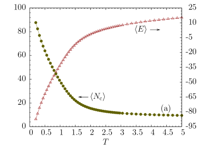
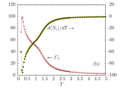
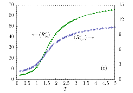
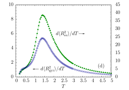
Figure 1: (a) Mean energy $\langle E\rangle$ and number of contacts $\langle N_{\mathrm{c}}\rangle$; (b) heat capacity $C_{\text{V}}$ and thermal fluctuation of the number of contacts $d\langle N_{\mathrm{c}}\rangle/dT$; (c) square end-to-end distance $\langle R^{2}_{\mathrm{ee}}\rangle$ and square radius of gyration $\langle R^{2}_{\mathrm{gyr}}\rangle$; (d) thermal fluctuations of the square end-to-end distance $d\langle R^{2}_{\mathrm{ee}}\rangle/dT$ and the square radius of gyration $d\langle R^{2}_{\mathrm{gyr}}\rangle/dT$ for a flexible polymer with 30 monomers. Error bars are smaller than the symbol size.

Integrated autocorrelation times can also be estimated by using the so-called binning method. Assuming that the time series consists of $N$ correlated measurements $O_{i}$, this time series can be divided into $K$ bins, which should be large enough so that the correlation of the data in each bins decays sufficiently ($N_{\mathrm{B}}\gg\tau_{O,\text{int}}$). In this way, a set of $K$ uncorrelated data subsets is generated, each of which contains $N_{\mathrm{B}}$ data points such that $N=N_{\mathrm{B}}K$. The binning block average $\overline{O}^{\mathrm{B}}_{k}$ of the $k$-th block is calculated as

$$\overline{O}^{\mathrm{B}}_{k}=\frac{1}{N_{\mathrm{B}}}\sum_{i=1}^{N_{\mathrm{B}}}O_{(k-1)N_{\mathrm{B}}+i},\quad k=1,\ldots,K,$$ (20)

and

$$\overline{O}=\frac{1}{K}\sum_{k=1}^{K}\overline{O}^{\mathrm{B}}_{k}\,,$$ (21)

coincides with the average (6). Since each bin average represents an independent measurement, the variance of the binning block averages $\sigma^{2}_{\overline{O}^{\mathrm{B}}}$ can be estimated from Eq. (17),

$$\tilde{\sigma}^{2}_{\overline{O}^{\mathrm{B}},\mathrm{c}}=\frac{1}{K-1}\sum_{k=1}^{K}\left(\overline{O}^{\mathrm{B}}_{k}-\overline{O}\right)^{2},$$ (22)

and the statistical error of the mean value $\epsilon^{2}_{\overline{O}}\equiv\sigma^{2}_{\overline{O}}=\sigma^{2}_{\overline{O}^{\mathrm{B}}}/K$ is given by

$$\epsilon^{2}_{\overline{O}}=\frac{\tilde{\sigma}^{2}_{\overline{O}^{\mathrm{B}},\mathrm{c}}}{K}=\frac{1}{K(K-1)}\sum_{k=1}^{K}\left(\overline{O}^{\mathrm{B}}_{k}-\overline{O}\right)^{2}.$$ (23)

By comparing this expression with Eq. (12) and considering Eqs. (11) and (13), we see that $\sigma^{2}_{\overline{O}^{\mathrm{B}}}/K=2\tau_{O,\text{int}}\sigma^{2}_{O}/N$. Hence, the autocorrelation time can also be estimated by means of the binning variance as

$$\tilde{\tau}_{O,\text{bin}}=\frac{1}{2}N_{\mathrm{B}}\frac{\tilde{\sigma}^{2}_{\overline{O}^{\mathrm{B}},\mathrm{c}}}{\tilde{\sigma}^{2}_{O}}.$$ (24)

Since the bin averages are supposed to be uncorrelated, we utilized the standard estimator (15) for the variance of the individual measurements $\sigma^{2}_{O}$ ($N\gg 2\tau_{O,\text{int}}$). This method is more convenient than the integration method (14) since a precise estimate of the autocorrelation function is not needed. For uncorrelated data and $N_{\mathrm{B}}=1$, $\tilde{\sigma}^{2}_{\overline{O}^{\mathrm{B}},\mathrm{c}}=\tilde{\sigma}^{2}_{O}$ for $N\gg 1$. Consequently $\tilde{\tau}_{O,\text{bin}}=\tau_{O,\text{int}}=1/2$. In the correlated case, too small bin sizes will underestimate the autocorrelation time. Given a time series consisting of $N$ measurements, the estimator $\tilde{\sigma}^{2}_{O}$ remains unchanged if $N_{\mathrm{B}}$ is modified. Increasing $N_{\mathrm{B}}$ reduces the number of bins $K$ which leads to the decrease of the variance $\tilde{\sigma}^{2}_{\overline{O}^{\mathrm{B}},\mathrm{c}}$. However, the decrease rate is not the same as $N_{\mathrm{B}}$ is increased. Thus, the right hand side of (24) will converge to a constant value identical to $\tau_{O,\text{int}}$. Therefore, one typically plots the right hand side of Eq. (24) for various values of $N_{\mathrm{B}}$ and estimates $\tau_{O,\text{int}}$ by reading the value the curve converges to WJanke2002 ; MBachmann .

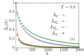
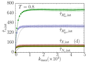
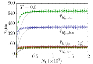
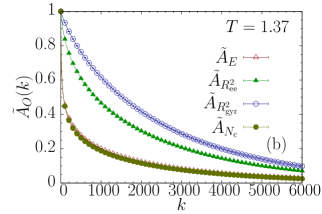
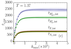
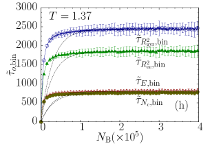
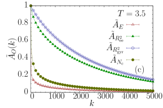
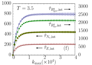
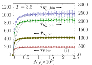
Figure 2: (a), (b), and (c) Autocorrelation functions of $E$, $R^{2}_{\mathrm{ee}}$, $R^{2}_{\mathrm{gyr}}$, and $N_{\mathrm{c}}$ at temperatures below, near, and above the collapse transition temperature, respectively, for $L=30$. For each quantity, the estimated integrated autocorrelation time converges to a constant as shown in (d), (e), and (f). The corresponding binning analysis results also show good convergence and are plotted in (g), (h), and (i). Dashed lines represent the fitted curves. Values of the fitted autocorrelation times the curves converge to are listed in Table 1.

III RESULTS

III.1 Autocorrelation times at constant displacement

For the interpretation of the autocorrelation times of energy, square end-to-end distance, square radius of gyration, and number of contacts, it is helpful to first investigate thermodynamic properties of these quantities. We have plotted the mean values of energy and number of contacts in Fig. 1(a), as well as the heat capacity and thermal fluctuation of the number of contacts in Fig. 1(b). A contact between two non-bonded monomers is formed, if their distance is in the interval $r_{ij}\in[0.8,1.2]$ for the 30-mer and $r_{ij}\in[0.87,1.13]$ for the 55-mer. The number of contacts is a simple discrete order parameter which is also helpful in distinguishing phases. It has proven to be particularly useful in studies of lattice models MBachmann2006-1 ; MBachmann2006-2 ; TVogel2007 . In the continuous model used here, it is a robust parameter that does not depend on energetic model details. Square end-to-end distance and square radius of gyration curves are shown in Fig. 1(c) and their thermal fluctuations in Fig. 1(d). The two clear peaks at $T\approx 1.4$ of the latter represent the collapse transition of the 30-mer. Note that the fluctuations of energy and contact number in Fig. 1(b) do not exhibit a peak at the transition point, but only a “shoulder”. As the temperature decreases, dissolved or random coils (gas phase) collapse in a cooperative arrangement of the monomers, and compact globular conformations (liquid phase) are favorably formed. As the temperature decreases further, the polymer transfers from the globular phase to the “solid” phase which is characterized by locally crystalline or amorphous metastable structures. A corresponding peak and valley which mark the liquid-solid (crystallization) or freezing transition of the 30-mer can be observed at $T\approx 0.28$ in the heat capacity and $d\langle N_{\mathrm{c}}\rangle/dT$ curves, respectively, in Fig. 1(b). These results coincide qualitatively with those of a previous study, where a slightly different model was employed Schnabel2011 . Due to insufficient Metropolis sampling at low temperatures, we did not include data in the $T<0.2$ region.

Table 1: Autocorrelation times of $E$, $R^{2}_{\mathrm{ee}}$, $R^{2}_{\mathrm{gyr}}$, and $N_{\mathrm{c}}$ estimated by integration of autocorrelation functions and by using the binning method at three temperatures below, near, and above the collapse transition.

$T$	$\tilde{\tau}_{E,\text{int}}$	$\tilde{\tau}_{E,\text{bin}}$	$\tilde{\tau}_{N_{\text{c}},\text{int}}$	$\tilde{\tau}_{N_{\text{c}},\text{bin}}$	$\tilde{\tau}_{R^{2}_{\text{ee}},\text{int}}$	$\tilde{\tau}_{R^{2}_{\text{ee}},\text{bin}}$	$\tilde{\tau}_{R^{2}_{\text{gyr}},\text{int}}$	$\tilde{\tau}_{R^{2}_{\text{gyr}},\text{bin}}$
0.8	122 $\pm$ 7	122 $\pm$ 13	$101\pm 7\enspace$	102 $\pm$ 13	696 $\pm$ 33	680 $\pm$ 75	427 $\pm$ 28	426 $\pm$ 50
1.37	810 $\pm$ 45	808 $\pm$ 94	763 $\pm$ 39	763 $\pm$ 93	1851 $\pm$ 103	1853 $\pm$ 201	2450 $\pm$ 138	2443 $\pm$ 272
3.5	209 $\pm$ 13	205 $\pm$ 25	446 $\pm$ 27	438 $\pm$ 52	2145 $\pm$ 106	2103 $\pm$ 228	2539 $\pm$ 121	2485 $\pm$ 268

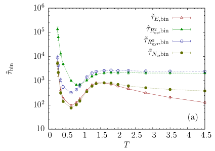
Figure 3: Temperature dependence of integrated autocorrelation times (a) estimated with the binning method; (b) obtained by the integration of autocorrelation functions for the 30-mer.

We performed the integration of the autocorrelation (14) and the binning analysis to estimate the integrated autocorrelation times at $17$ temperatures in the interval $T\in[0.26,4.5]$ for the 30-mer and at $16$ temperatures in the interval $T\in[0.3,5]$ for the 55-mer. Mean values $\overline{Q}_{O}(x)$ (where $\overline{Q}_{O}(x)$ stands for $\overline{\tilde{A}}_{O}(k)$, $\overline{\tilde{\tau}}_{O,\text{bin}}(N_{\mathrm{B}})$ or $\overline{\tilde{\tau}}_{O,\text{int}}(k_{\text{max}})$) for a quantity $O$ were calculated at each temperature in $N_{\mathrm{r}}$ ($N_{\mathrm{r}}>20$) independent runs:

$$\overline{Q}_{O}(x)=\frac{1}{N_{\mathrm{r}}}\sum_{i=1}^{N_{\mathrm{r}}}Q_{O}^{i}(x),$$ (25)

where $Q_{O}^{i}(x)$ is the value calculated in the $i$th run. As shown in Fig. 2, all estimates of autocorrelation functions and times converge for large values of $k$, $k_{\text{max}}$, and $N_{\mathrm{B}}$, respectively, as expected. The error of $\overline{Q}_{O}(x)$ is estimated by

$$\epsilon^{2}_{\overline{Q}_{O}(x)}=\frac{1}{N_{\mathrm{r}}-1}\sum_{i=1}^{N_{\mathrm{r}}}\left(Q^{i}_{O}(x)-\overline{Q}_{O}(x)\right)^{2},$$ (26)

because all runs were performed independently of each other. The consistency of the two different methods used for the estimation of autocorrelation times for the investigated quantities become apparent from Table 1, where we have listed the autocorrelation time estimate for three temperatures below, near, and above the $\Theta$ point. The results coincide within the numerical error bars.

In order to estimate the integrated autocorrelation time systematically, we performed least-squares fitting for all the curves in both the integration method of the autocorrelation function and binning analysis at each temperature. The empirical fit function for any quantity $O$ is chosen to be of the form

$$f_{O}(x)=\tau^{f}_{O}(1-e^{-x/x^{f}}),$$ (27)

where $x$ represents $k_{\text{max}}$ in the integration of the autocorrelation functions method and $N_{\mathrm{B}}$ in binning analysis; $\tau^{f}_{O}$ and $x^{f}$ are two fit parameters. The fitting curves, also plotted in Fig. 2, coincide well with the mean values of the integrated autocorrelation times in the $N_{\mathrm{B}}/k_{\text{max}}$ region, where convergence sets in.

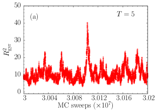
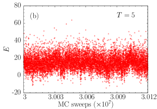
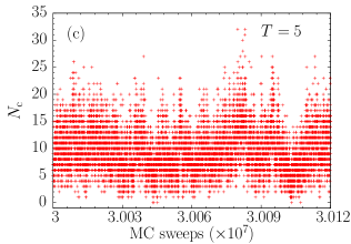
Figure 4: (a), (b), and (c) are parts of the time series of $R^{2}_{\mathrm{gyr}}$, $E$, and $N_{\mathrm{c}}$ at $T=5$ in equilibrium for the 30-mer.

It is necessary to mention that when using the binning method to calculate error bars one needs to ensure that the binning block length is much larger than the autocorrelation time. The reason is obvious from Fig. 2. If the autocorrelation time estimated by the binning method has not yet converged, the estimate $\tilde{\tau}_{O,\text{bin}}$ is less than the integrated autocorrelation time ($\tilde{\tau}_{O,\text{bin}}<\tau_{O,\text{int}}$). Therefore, the estimated standard deviation

$$\epsilon^{2}_{\overline{O}}=\frac{\tilde{\sigma}^{2}_{\overline{O}^{\mathrm{B}},\mathrm{c}}}{K}=\frac{2\tilde{\sigma}^{2}_{O}}{N}\tilde{\tau}_{O,\text{bin}}$$ (28)

underestimates the true value $\epsilon^{2}_{\overline{O}}=2\sigma^{2}_{O}\tau_{O,\text{int}}/N$ in this case, yielding a too small error estimate.

After the preliminary considerations, we will now discuss how the dependence of the autocorrelation time on the temperature can be utilized for the identification of structural transitions in the polymer system.

III.2 Slowing down at the $\Theta$ point

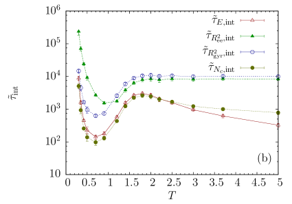
Figure 5: Same as Fig. 3, but for the 55-mer.

Figure 3 shows how the fitted estimated integrated autocorrelation times $\tau^{f}_{O}$ vary with temperature. As the comparison shows, the autocorrelation times estimated by using the binning analysis are in very good agreement with the results obtained by integrating autocorrelation functions.

The integrated autocorrelation time curves of $R^{2}_{\mathrm{ee}}$ and $R^{2}_{\mathrm{gyr}}$ behave similarly at most of the temperatures except the temperatures close to the freezing transition. This is not surprising as both are structural quantities that are defined to describe the compactness of the polymer. In addition, the integrated autocorrelation time curves of $E$ and $N_{\mathrm{c}}$ behave similarly. Their relation can be understood as following. The polymer conformation in the solid phase is characterized by locally crystalline or amorphous metastable structures. Therefore, the main contribution of each monomer to the energy in this phase originates from the interaction between this monomer and its non-bonded nearest neighbors. This is also reflected by the number of contacts to the nearest neighbors. Thus, $E\propto N_{\mathrm{c}}$ in the solid phase (see Fig. 1(a)). The autocorrelation times of the two structural quantities are always larger than the ones of $E$ and $N_{\mathrm{c}}$. The reason is that these quantities are not particularly sensitive to conformational changes within a single phase. Furthermore, the displacement update used here does not allow for immediate substantial changes. This can be seen in Fig. 4(a) where the time series are shown at high temperature. From Fig. 4(b) and 4(c), one notices that $E$ and $N_{\mathrm{c}}$ fluctuate more strongly than $R^{2}_{\mathrm{gyr}}$.

The most important observation from Fig. 3 is that slowing down appears near $T\approx 1.4$ which signals the collapse transition. This temperature is close to the peak positions of the structural fluctuations shown in Fig. 1(d). Within this temperature region, the autocorrelation time becomes extremal. Large parts of the polymer have to behave cooperatively which slows down the overall collapse dynamics.

Near the freezing transition ($T\approx 0.3$), the autocorrelation times of all four quantities rapidly increase. Since Metropolis simulations with local updates typically get stuck in metastable states of the polymer at low temperatures, we do not estimate autocorrelation times in the $T<0.26$ region. The freezing transition is, therefore, virtually inaccessible to any autocorrelation time analysis based on local-update Metropolis simulations. This is amplified by the fact that the autocorrelation time increase naturally at low temperatures, because of the low entropy. That means if there would be a signal of the freezing transition at all in the autocorrelation time curves, it would be difficult to identify it.

The autocorrelation times of $R^{2}_{\mathrm{ee}}$, $R^{2}_{\mathrm{gyr}}$, and $N_{\mathrm{c}}$ seem to converge to constant values at high temperatures, whereas the autocorrelation time of $E$ decays. This is partly due to the fact that the structural quantities and $N_{\mathrm{c}}$ possess upper limiting values that are reached at high temperatures, thereby reducing the fluctuation width at constant displacement range. This is a particular feature of the results obtained in simulations with fixed maximum displacement and it is different if the acceptance rate is kept constant instead. This will be discussed in Sec. III.3.

The overall behavior is similar to Metropolis dynamics for the two-dimensional Ising model on the square lattice, in which the external field is excluded so that $E\in[-2JL^{2},2JL^{2}]$ where $J>0$ is the coupling constant and $L$ is the lattice size and $M\in[-L^{2},L^{2}]$ NewmanMC1999 .

In order to verify that the general autocorrelation properties apply also to larger polymers, we repeated the simulations for a 55-mer. From Fig. 5, we notice that the behavior is qualitatively the same, but the autocorrelation times of all quantities are larger than the ones for the 30-mer, as expected. This supports our hypothesis that the qualitative behavior of the autocorrelation times of the 30-mer is generic and representative for autocorrelation properties of larger polymers. In particular, this method offers a possible way for the identification of transitions, where standard canonical analysis of quantities such as the specific heat fails.

III.3 Autocorrelation times at a fixed acceptance rate

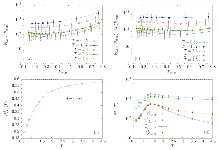
Figure 6: (a) Integrated autocorrelation times of the energy $\tilde{\tau}_{E,\text{bin}}$ at different acceptance rates $P_{\text{accp}}$ for various temperatures near the collapse transition of the 30-mer; (b) modified autocorrelation times of energy versus acceptance rates; (c) acceptance rates at fixed maximum displacement $d=0.3r_{0}$ for different temperatures; (d) integrated autocorrelation times at fixed acceptance rate $P^{\mathrm{\,a}}_{\mathrm{accp}}=0.2$ as a function of temperature for the 30-mer.

In order to find out how the autocorrelation time changes at a fixed acceptance rate rather than at a fixed maximum displacement range, we used the binning method to calculate the integrated autocorrelation times at different constant acceptance rates $P_{\text{accp}}$ for different temperatures near the collapse transition for the 30-mer. The results for the energetic autocorrelation times $\tilde{\tau}_{E,\mathrm{bin}}(P_{\mathrm{accp}})$ are shown in Fig. 6(a), measured for five different temperatures. Autocorrelation times of the other quantities exhibit a similar behavior. Two important conclusions can be drawn: (i) the values of the autocorrelation times depend on acceptance rate and temperature, but (ii) the monotonic behavior of $\tilde{\tau}_{E,\mathrm{bin}}$ as a function of $P_{\mathrm{accp}}$ is virtually independent of the temperature. Thus, if multiplied by a temperature-independent empirical modification factor

$$M(P_{\text{accp}})=e^{-4|P_{\text{accp}}-0.2|^{1.65}},$$ (29)

the modified autocorrelation time curves become almost independent of $P_{\mathrm{accp}}$ at these temperatures (see Fig. 6(b)):

$$\tilde{\tau}_{\text{bin}}(P_{\mathrm{accp}})\cdot M(P_{\mathrm{accp}})\approx\mathrm{const.}$$ (30)

in the interval $P_{\mathrm{accp}}\in(0.14,0.78)$. This feature of uniformity in monotonic behavior and the empirical modification factor (29) can then be used to modify the autocorrelation times at all temperatures. For this purpose one reads the autocorrelation time $\tilde{\tau}^{\mathrm{d}}_{\mathrm{bin}}(T)$ and the acceptance rate $P^{\mathrm{\,d}}_{\mathrm{accp}}(T)$ at fixed maximum displacement at a given temperature $T$ from Fig. 3(a) and Fig. 6(c), respectively, calculates the modification factor $M(P^{\mathrm{\,d}}_{\mathrm{accp}}(T))$ from Eq. (29), and obtains the modified autocorrelation time $\tilde{\tau}^{\mathrm{a}}_{\mathrm{bin}}$ at constant acceptance rate $P^{\mathrm{\,a}}_{\mathrm{accp}}$ by making use of Eq. (30). For simplicity, we choose $P^{\mathrm{\,a}}_{\mathrm{accp}}=0.2$, which yields

$$\tilde{\tau}^{\mathrm{a}}_{\text{bin}}(T)=\tilde{\tau}^{\mathrm{d}}_{\text{bin}}(T)\cdot M(P^{\mathrm{\,d}}_{\mathrm{accp}}(T)),$$ (31)

since $M(0.2)=1$. The temperature dependence of this modified autocorrelation time is shown in Fig. 6(d). One notices that the peaks indicating the collapse transition are more pronounced than the ones in the fixed maximum displacement case, but qualitatively (and quantitatively regarding the $\Theta$ transition point) this modified approach leads to similar results. In the temperature range investigated here, the autocorrelation times of all quantities seem to decrease above the $\Theta$ point. This is different than the behavior at fixed maximum displacement range (cp. Fig. 3(a)).

IV SUMMARY

Employing the Metropolis Monte Carlo algorithm, we have performed computer simulations of a simple coarse-grained model for flexible, elastic polymers to investigate the autocorrelation time properties for different quantities. Two different methods were employed to estimate autocorrelation times as functions of temperatures for polymers with 30 and 55 monomers: by integration of autocorrelation functions and by using the binning method. The results obtained for different energetic and structural quantities by averaging over more than 20 independent simulations are consistent.

The major result of our study is that autocorrelation time changes can be used to locate structural transitions of polymers, because of algorithmic slowing down. We deliberately employed Metropolis sampling and local displacement updates, as slowing down is particularly apparent in this case. We could clearly identify the collapse transition point for the two chain lengths investigated. Low-temperature transitions are not accessible because of the limitations of Metropolis sampling in low-entropy regions of the state space.

The identification of transitions by means of autocorrelation time analysis is, therefore, an alternative and simple method to more advanced technique such as microcanonical analysis MBachmann ; Gross2001 ; Janke1998 ; Behringer2006 ; Schnabel2011 or by investigating partition function zeros YangLee ; Fisher1965 ; Janke2001-2002 ; JRocha . Those methods require the precise estimation of the density of states of the system which can only be achieved in sophisticated generalized-ensemble simulations. The autocorrelation time analysis method is very robust and can be used as an alternative method for the quantitative estimation of transition temperatures, in particular, if the more qualitative standard canonical analysis of “peaks” and “shoulders” in fluctuating quantities remains inconclusive.

- (1) P.H. Verdier and W.H. Stockmayer, J. Chem. Phys. 36, 227 (1962).
- (2) P.H. Verdier, J. Chem. Phys. 45, 2122 (1966).
- (3) D.E. Kranbuehl and P.H. Verdier, J. Chem. Phys. 56, 3145 (1972).
- (4) P.H. Verdier, J. Chem. Phys. 59, 6119 (1973).
- (5) D.E. Kranbuehl, P.H. Verdier, and J.M. Spencer, J. Chem. Phys. 59, 3861 (1973).
- (6) D.E. Kranbuehl and P.H. Verdier, J. Chem. Phys. 67, 361 (1977).
- (7) J.A. McCormick, C.K. Hall, and S.A. Khan, J. Chem. Phys. 122, 114902 (2005).
- (8) E.M. Pestryaev, J. Phys.: Conf. Ser. 324, 012031 (2011).
- (9) T. Aoyagi, J. Takimoto, and M. Doi, J. Chem. Phys. 115, 552 (2001).
- (10) A. Malevanets and J.M. Yeomans, Europhys. Lett. 52, 231 (2000).
- (11) J.M. Polson and J.P. Gallant, J. Chem. Phys. 124, 184905 (2006).
- (12) M. Bishop, M.H. Kalos, and H.L. Frisch, J. Chem. Phys. 70, 1299 (1979).
- (13) D.C. Rapaport, J. Chem. Phys. 71, 3299 (1979).
- (14) W. Bruns and R. Bansal, J. Chem. Phys. 74, 2064 (1981).
- (15) W. Bruns and R. Bansal, J. Chem. Phys. 75, 5149 (1981).
- (16) K. Mussawisade, M. Ripoll, R.G. Winkler, and G. Gompper, J. Chem. Phys. 123, 144905 (2005).
- (17) P.P. Nidras and R. Brak, J. Phys. A: Math. Gen. 30, 1457 (1997).
- (18) D.P. Landau and K. Binder, A Guide to Monte Carlo Simulations in Statistical Physics (Cambridge University Press, Cambridge, 2000).
- (19) M.E.J. Newman and G.T. Barkema, Monte Carlo Methods in Statistical Physics, (Oxford University Press, Oxford, 1999).
- (20) W. Janke, Statistical Analysis of Simulations: Data Correlations and Error Estimation, in Proceedings of the Winter School “Quantum Simulations of Complex Many-Body Systems: From Theory to Algorithms”, John von Neumann Institute for Computing, Jülich, NIC Series vol. 10, ed. by J. Grotendorst, D. Marx and A. Muramatsu (NIC, Jülich, 2002), p. 423.
- (21) W. Janke, Monte Carlo Simulations of Spin Systems, in: Computational Physics: Selected Methods Simple Exercises Serious Applications, eds. K.H. Hoffmann and M. Schreiber (Springer, Berlin, 1996), p. 10.
- (22) W. Janke, Nonlocal Monte Carlo Algorithms for Statistical Physics Applications, Mathematics and Computers in Simulations 47, 329 (1998).
- (23) N. Metropolis, A.W. Rosenbluth, M.N. Rosenbluth, A.H. Teller, and E. Teller, J. Chem. Phys. 21, 1087 (1953).
- (24) A.D. Sokal, Monte Carlo Methods in Statistical Mechanics: Foundations and New Algorithms, lecture notes, Cours de Troisième Cycle de la Physique en Suisse Romande, Lausanne, 1989.
- (25) A.D. Sokal, Bosonic Algorithms, in: Quantum Fields on the Computer, ed. M. Creutz (World Scientific, Singapore, 1992), p. 211.
- (26) M.P. Nightingale and H.W.J. Blöte, Phys. Rev. Lett. 76, 4548 (1996).
- (27) R. Matz, D.L. Hunter, and N. Jan, J. Stat. Phys. 74, 903 (1994).
- (28) P.D. Coddington and C.F. Baillie, Phys. Rev. Lett. 68, 962 (1992).
- (29) D. Kandel, E. Domany, D. Ron, A. Brandt, and E. Loh, Phys. Rev. Lett. 60, 1591 (1988).
- (30) D. Kandel, E. Domany, and A. Brandt, Phys. Rev. B 40, 330 (1989).
- (31) J.D. Gunton, M.S. Miguel, and P.S. Sahni, The Dynamics of First Order Phase Transitions in: Phase Transitions and Critical Phenomena, Vol. 8, eds. C. Domb and J.L. Lebowitz (Academic Press, New York, 1983), p. 269.
- (32) K. Binder, Rep. Prog. Phys. 50, 783 (1987).
- (33) H.J. Herrmann, W. Janke, and F. Karsch (eds.), Dynamics of First Order Phase Transitions (World Scientific, Singapore, 1992).
- (34) W. Janke, Recent Developments in Monte Carlo Simulations of First-Order Phase Transitions, in: Computer Simulations in Condensed Matter Physics VII, eds. D.P. Landau, K.K. Mon and H.-B. Schüttler (Springer, Berlin, 1994), p. 29.
- (35) W. Janke, First-Order Phase Transitions, in: Computer Simulations of Surfaces and Interfaces, NATO Science Series, II. Mathematics, Physics and Chemistry - Vol. 114, Proceedings of the NATO Advanced Study Institute, Albena, Bulgaria, 9 - 20 September 2002, edited by B. Dünweg, D.P. Landau, and A.I. Milchev (Kluwer, Dordrecht, 2003); pp. 111 - 135.
- (36) B.A. Berg and T. Neuhaus, Phys. Lett. B267, 249 (1991); Phys. Rev. Lett. 68, 9 (1992).
- (37) W. Janke, B.A. Berg, and M. Katoot, Nucl. Phys. B382, 649 (1992).
- (38) B.A. Berg, U. Hansmann, and T. Neuhaus, Phys. Rev. B 47, 497 (1993); Z. Phys. B 90, 229 (1993).
- (39) A. Billoire, T. Neuhaus, and B.A. Berg, Nucl. Phys. B 396, 779 (1993).
- (40) B. Grossmann and M.L. Laursen, Int. J. Mod. Phys. C3, 1147 (1992); Nucl. Phys. B 408, 637 (1993).
- (41) W. Janke and T. Sauer, Phys. Rev. E 49, 3475 (1994).
- (42) M. Bachmann, Thermodynamics and Statistical Mechanics of Macromolecular Systems, (Cambridge University Press, Cambridge, 2014).
- (43) R.B. Bird, C.F. Curtiss, R.C. Armstrong, and O. Hassager, Dynamics of Polymeric Liquids, 2nd ed. (Wiley, New York, 1987).
- (44) A. Milchev, A. Bhattacharya, and K. Binder, Macromolecules 34, 1881 (2001).
- (45) M. Bachmann and W. Janke, Phys. Rev. E 73, 020901(R) (2006).
- (46) M. Bachmann and W. Janke, Phys. Rev. E 73, 041802 (2006).
- (47) T. Vogel, M. Bachmann, and W. Janke, Phys. Rev. E 76, 061803 (2007).
- (48) D.H.E. Gross, Microcanonical Thermodynamics (World Scientific, Singapore, 2001).
- (49) W. Janke, Nucl. Phys. B, Proc. Suppl. 63A-C, 631 (1998).
- (50) H. Behringer and M. Pleimling, Phys. Rev. E 74, 011108 (2006).
- (51) S. Schnabel, D.T. Seaton, D.P. Landau, and M. Bachmann, Phys. Rev. E 84, 011127 (2011).
- (52) C.N. Yang and T.D. Lee, Phys. Rev. 87, 404 (1952); T.D. Lee and C.N. Yang, Phys. Rev. 87, 410 (1952).
- (53) M.E. Fisher, in Lectures in Theoretical Physics vol. 7C, ed. by W.E. Brittin (University of Colorado Press, Boulder, 1965), Chap. 1.
- (54) W. Janke and R. Kenna, J. Stat. Phys. 102, 1211 (2001); Comp. Phys. Comm. 147, 443 (2002); Nucl. Phys. B (Proc. Suppl.) 106-107, 905 (2002).
- (55) J.C.S. Rocha, S. Schnabel, D.P. Landau, and M. Bachmann, Phys. Rev. E, in press (2014).