Importance of anisotropic exchange interactions in honeycomb iridates. Minimal model for zigzag antiferromagnetic order in Na₂IrO₃.

Abstract

In this work, we investigate the microscopic nature of the magnetism in honeycomb iridium-based systems by performing a systematic study of how the effective magnetic interactions in these compounds depend on various electronic microscopic parameters. We show that the minimal model describing the magnetism in A₂IrO₃ includes both isotropic and anisotropic Kitaev-type spin-exchange interactions between nearest and next-nearest neighbor Ir ions, and that the magnitude of the Kitaev interaction between next-nearest neighbor Ir magnetic moments is comparable with nearest neighbor interactions. We also find that, while the Heisenberg and the Kitaev interactions between nearest neighbors are correspondingly antiferro- and ferromagnetic, they both change sign for the next-nearest neighbors. Using classical Monte Carlo simulations we examine the magnetic phase diagram of the derived super-exchange model. Zigzag-type antiferromagnetic order is found to occupy a large part of the phase diagram of the model and, for ferromagnetic next-nearest neighbor Heisenberg interaction relevant for Na₂IrO₃, it can be stabilized even in the absence of third nearest neighbor coupling. Our results suggest that a natural physical origin of the zigzag phase experimentally observed in Na₂IrO₃ is due to the interplay of the Kitaev anisotropic interactions between nearest and next-nearest neighbors.

I Introduction

The magnetism in $4d$ and $5d$ transition metal (TM) oxides, particularly realized in iridates and rhodates, has recently attracted a lot of interest. In these systems, the interplay between the spin-orbit (SO) coupling, the crystal field (CF) splitting, and Coulomb and Hund’s coupling leads to a rich variety of magnetic exchange interactions, new types of magnetic ground states and excitations.

In our recent workperkins14 (hereafter referred to as paper I), we applied the Mott insulator scenario, extending the original study by Jackeli and Khalliulin, jackeli09 and developed a theoretical framework for the derivation of effective super-exchange Hamiltonians that govern the magnetic properties of systems with strong SO coupling. In our approach, both the many-body (Coulomb and Hund’s interaction) and the single electron (SO and CF interactions) effects are treated on an equal footing. In this framework, we first determined the localized degrees of freedom of the iridium system by finding the exact eigenstates of the single-ion microscopic Hamiltonian for Ir⁴⁺ ions, and then computed the interactions between them. Because of time reversal symmetry of the single-ion Hamiltonian, the lowest atomic state is always at least two-fold degenerate, and can be described using pseudospin-$1/2$ operators.

In paper I, some of us showed that the super-exchange Hamiltonian describing interactions between these pseudospins might have unusual anisotropic components. Moreover, these anisotropic interactions might be the dominating interactions between magnetic moments. The form of these anisotropic interactions may also be quite unusual. In particular, they do not need to be confined to the traditional anisotropic interaction types acting equally on all sites of the lattice (i.e. easy-plane or easy-axis anisotropy). Instead, the anisotropic interactions might involve coupling between different components of spins sitting on different lattice sites. The Dzyaloshinskii-Moriya interactiondzyalo58 ; moriya60 and the Kitaev interaction on the honeycomb latticekitaev06 ; jackeli10 are salient examples of such interactions.

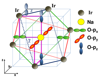
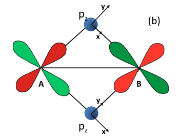
Figure 1: (Colors online) (a) Schematic representation of A₂IrO₃ structure. $x-$, $y-$ and $z-$ n.n. Ir-Ir bonds are shown by red, green and blue solid lines. ${\tilde{x}}-$, ${\tilde{y}}-$ and ${\tilde{z}}-$ second n. n. Ir-Ir bonds are shown by red, green and blue dotted lines. Thick magenta lines represents Ir-O-Na-O-Ir second n. n. super-exchange paths. (b) Undistorted 90^∘ Ir-O-Ir bond. Local axes for Ir⁴⁺ ions on A and B sublattices are the same as the global axes. Two possible super-exchange paths via upper or lower oxygen are shown.

In paper I, we focused on iridates and rhodates with tetragonal symmetry, e.g. we studied in detail the magnetic interactions in Sr₂IrO₄. cao98 ; bjkim08 ; moon09 ; kim09 ; comin12 ; fujiyama14 Our approach allowed us to show that the weak coplanar ferromagnetism observed in Sr₂IrO₄cao98 is governed by the Dzyaloshinskii-Moriya interaction with an unusual strength owing to the large SO coupling. In the present paper, we make use of the experience obtained in paper I to study the magnetic properties of A₂IrO₃ singh10 ; singh12 ; liu11 ; ye12 ; choi12 (A=Na,Li) in which the Ir⁴⁺ ions occupy the sites of a honeycomb lattice.

The nearest-neighbor (n. n.) super-exchange in honeycomb iridates in the absence of lattice distortions, the so-called Kitaev-Heisenberg (KH) model, was first proposed by Jackeli and Khalliulin. jackeli09 ; jackeli10 They showed that in these systems the coupling between n. n. Ir magnetic moments occurs through both direct exchange between Ir⁴⁺ ions and through a super-exchange coupling mediated by an intermediate oxygen along the 90^∘ Ir-O-Ir bond. The latter process gives rise to a nonzero anisotropic interaction between pseudospins, which has the form of the aforementioned Kitaev interactions, but only for a finite value of the Hund’s coupling. The KH model correctly captures the nature of the anisotropic part of the magnetic interactions in Na₂IrO₃ honeycomb compounds and also predicts some non-trivial properties of these compounds at finite temperatures. price12 ; price13 Nevertheless, the model does miss some essential features: it does not account for both the zigzag magnetic order and for the spectrum of magnetic excitations in Na₂IrO₃ measured in neutron scattering experiments. liu11 ; ye12 ; choi12 Partly, this is because the original KH model neither includes further neighbor interactions, which have been shown to play a significant role in stabilizing the zigzag antiferromagnetic ordering in Na₂IrO₃, kimchi11 ; choi12 nor lattice distortions, which might also be essential for these compounds.

In this work we revisit the KH modeljackeli09 ; jackeli10 and derive its extension up to second neighbor’s interactions, starting from the exact eigenstates of the single-ion microscopic Hamiltonian which equally includes both the SO coupling and the trigonal distortion. In this context, our work differs from the recent study by Bhattacharjee, Lee and Kim, subhro12 in which the effective spin Hamiltonian was derived by setting the energy scale associated with trigonal distortion to infinity first, followed by that of the SO energy scale. Here, we estimate the strength of magnetic interactions in Na₂IrO₃ based on the tight-binding parameters obtained from the ab-initio density-functional theory study by Foyevtsova et al.katerina13 We show that the effective spin Hamiltonian on the honeycomb lattice, whose bonding geometry is shown in Fig. 1 (a), contains several anisotropic spin interactions among which the strongest is the Kitaev interaction between nearest neighbors.

We also compute the super-exchange interaction between the second neighbors forming two triangular sublattices, and find that it is of a form similar to the n. n. interaction, i.e. the dominant part can be written as a sum of isotropic Heisenberg and anisotropic Kitaev terms. These interactions are only slightly smaller than the n. n. Kitaev interactions. Other anisotropic interactions, which couple different components of spins on a given bond, are significantly smaller and most of them are non-zero only in the presence of trigonal lattice distortions. In this respect they are different from the Kitaev-like interactions which are present even in the ideal structure.

The magnetic phase diagram which emerges from our study is presented in Fig. 5. This is the key result of this paper. We argue that the zigzag magnetic order, experimentally observed in Na₂IrO₃, is stabilized by the interplay of four major interactions: isotropic antiferromagnetic and anisotropic ferromagnetic Kitaev interactions for n. n. bonds, isotropic ferromagnetic and anisotropic antiferromagnetic Kitaev interactions for the next-nearest neighbors. Unlike in other theoretical studies of magnetic properties of Na₂IrO₃kimchi11 ; jackeli13 ; katukuri14 , in our model the zigzag phase is stabilized for both the correct signs of n. n. interactions, and even without invoking third neighbor interactions.

The rest of the paper is organized as follows. In Sec. II, we introduce the single ion microscopic model appropriate for the description of the physical properties of iridates on the honeycomb lattice. We first obtain one-particle eigenstates taking into account only SO coupling and trigonal CF interaction. We then compute two-particle excited eigenstates fully considering correlation effects. Then, in Sec. III, we briefly review the derivation of an effective super-exchange Hamiltonian for these systems. All technical details of the derivation can be found in our previous work.perkins14 In Sec. IV, we obtain hopping matrices for neighboring iridium ions. Our calculation is based on a tight-binding fitting of ab-initio electronic structure in the presence of trigonal distortion performed by Foyevtsova et al.katerina13 In Sec. V, we present our results on the magnetic interactions. We show that these interactions can be most generally represented by a $3\times 3$ bond-dependent exchange coupling matrix. We show that, while the Kitaev-type of anisotropy is determined by the inequality of its diagonal elements due to the Hund’s coupling, the off-diagonal matrix elements are anisotropies mostly caused by the trigonal crystal field. In Sec. VI, taking into account only the dominant interactions, we perform classical Monte Carlo simulations and obtain the low-temperature phase diagram of the minimal super-exchange model for honeycomb iridates. We conclude in Sec. VII with a summary and discussion of our results.

II Single-ion Hamiltonian

II.1 One-particle eigenstates

In all iridates considered here, the Ir⁴⁺ ions sit inside an oxygen cage forming an octahedron. This octahedral CF splits the five 5$d$ orbitals of Ir⁴⁺ into doubly degenerate $e_{g}$ orbitals at higher energy and into the three-fold degenerate $t_{2g}$ multiplet. In iridates, the energy difference between $e_{g}$ and $t_{2g}$ levels is large and is typically of the order 2-3 eV. Because of this, the five electrons occupy only the low lying $t_{2g}$ orbitals. As a consequence, the on-site interactions, such as the SO, Coulomb and Hund’s interactions, as well as additional symmetry-lowering CF interactions, e.g. the trigonal CF, can be considered within the $t_{2g}$ manifold only. In this limit of large octahedral CF, the SO coupling has to be projected onto the $t_{2g}$ manifold, assuming an effective orbital angular momentum $L=1$. In terms of local axes, which are bound to the oxygen octahedron, the $t_{2g}$ orbitals of Ir ions are $\left|X\right\rangle\equiv\left|yz\right\rangle$, $\left|Y\right\rangle\equiv\left|zx\right\rangle$, and $\left|Z\right\rangle\equiv\left|xy\right\rangle$. The SO and trigonal CF interactions give rise to a splitting of the levels according to the symmetry of the underlying lattice. In the case of the honeycomb iridates, A₂IrO₃, the trigonal CF arises from a compression of the oxygen cages along the $[111]$ directions (local $C_{3}$ axis). At ambient pressure, the splitting of the $t_{2g}$ levels due to the trigonal CF is about 110 meV gret13 which is smaller, but of the same order of magnitude as the SO coupling, which is about 400 meV. Therefore, here we treat the SO coupling and the trigonal CF interactions on the same footing. Also, it is believed that much larger values of the trigonal distortion can be reached by applying uniaxial pressure.

Since the Hamiltonian is time-reversal invariant, the ground-state of the single-ion single-hole ($5d^{5}$ configuration of Ir⁴⁺ ion) is a Kramer’s doublet, which we represent as a pseudospin-1/2. However, the choice of the two orthonormal states within the doublet that would represent the pseudospin-up and pseudospin-down states deserves some well-inspired consideration, as this choice determines the coordinate system of the final super-exchange Hamiltonian. Since the most prominent anisotropy, the Kitaev interaction, has the simplest form in the coordinate system bound to the cubic axes of the oxygen octahedron environment, we choose the two orthogonal states that correspond to this particular Cartesian reference frame. In the absence of the trigonal distortion, the ground state doublet is simply a $J_{\rm eff}=1/2$ doublet and the good choice of the states within it are the $J_{\rm eff}^{z}=\pm 1/2$ states. In the presence of the trigonal distortion, the choice of the representation is not as straightforward since the ground state doublet contains a mixture of both $J_{\rm eff}=1/2$ and $J_{\rm eff}=3/2$ states. To resolve this, we first find a random set of orthonormal states within the doublet and then make linear combinations of them in such a way that pseudospin-1/2 ”up-state” has no $\left|J_{\rm eff}=1/2,J_{\rm eff}^{z}=-1/2\right\rangle$ component, whereas pseudospin-1/2 ”down-state” has no $\left|J_{\rm eff}=1/2,J_{\rm eff}^{z}=1/2\right\rangle$ component. Namely, we allow the trigonal CF to admix the $J_{\rm eff}=3/2$ states to the $J_{\rm eff}=1/2$ states, but we do not allow the latter to mix among themselves.

In the most simple form, the single-ion Hamiltonian can be written when the axis of the quantization of angular momentum is along the $[111]$ direction:

$$H_{\lambda,\Delta}=\lambda{\mathbf{S}}\cdot{\mathbf{L}}+\Delta L_{[111]}^{2},$$ (1)

where $L_{[111]}$ denotes the component of the angular momentum along the $[111]$ axis. Here the first term describes the SO coupling and the second term describes the trigonal CF. However, this form is not useful if we want to obtain our final result in the Cartesian reference frame bounded to the cubic crystallographic axes. If now we rewrite the CF term in terms of it’s eigenstates, then the Hamiltonian (1) becomes:

$$H_{\lambda,\Delta}=\lambda{\mathbf{S}}\cdot{\mathbf{L}}+\frac{\Delta}{3}\left(-2|a_{1g}\rangle\langle a_{1g}|+|e_{g}^{+}\rangle\langle e_{g}^{+}|+|e_{g}^{-}\rangle\langle e_{g}^{-}|\right),$$ (2)

where the crystal field eigenstates include the low-energy singlet $|a_{1g}\rangle$ and the higher energy doublet $|e_{g}^{\pm}\rangle$. The singlet state can be written as

$$|a_{1g}\rangle=\hat{\nu}_{x}|X\rangle+\hat{\nu}_{y}|Y\rangle+\hat{\nu}_{z}|Z\rangle,$$ (3)

where $\hat{\bm{\nu}}=(\hat{\nu}_{x},\hat{\nu}_{y},\hat{\nu}_{z})$ is the unit vector parallel to the $[111]$ trigonal axis ($\hat{\nu}_{j}=1/\sqrt{3}$). The doublet state can be conveniently written using the following chiral basis:

$$\begin{array}[]{c}|e_{g}^{+}\rangle=\hat{\nu}_{x}e^{-i\omega}|X\rangle+\hat{\nu}_{y}e^{+i\omega}|Y\rangle+\hat{\nu}_{z}|Z\rangle,\\ |e_{g}^{-}\rangle=\hat{\nu}_{x}e^{+i\omega}|X\rangle+\hat{\nu}_{y}e^{-i\omega}|Y\rangle+\hat{\nu}_{z}|Z\rangle,\end{array}$$ (6)

where $\omega\equiv 2\pi/3$. Now, that the CF part of the Hamiltonian is written in an $L$-independent way, we are free to choose the angular momentum quantization axis along the cubic $z$ direction for our basis. The basis we use is ${\hat{J}}=\{|\frac{1}{2},\frac{1}{2}\rangle,|\frac{1}{2},-\frac{1}{2}\rangle,|\frac{3}{2},\frac{3}{2}\rangle,|\frac{3}{2},\frac{1}{2}\rangle,|\frac{3}{2},-\frac{1}{2}\rangle,|\frac{3}{2},-\frac{3}{2}\rangle\}$. The details of this basis and its relation to the basis of the cubic orbitals are given in paper I.perkins14 The Hamiltonian matrix in this basis is given by

$${\hat{H}}=\left(\begin{array}[]{cccccc}-\lambda&0&-\frac{(1-\imath)\Delta}{3\sqrt{6}}&0&\frac{(1+\imath)\Delta}{3\sqrt{2}}&\frac{\imath\Delta}{3}\sqrt{\frac{2}{3}}\\ 0&-\lambda&\frac{\imath\Delta}{3}\sqrt{\frac{2}{3}}&\frac{(1-\imath)\Delta}{3\sqrt{2}}&0&-\frac{(1+\imath)\Delta}{3\sqrt{6}}\\ -\frac{(1+\imath)\Delta}{3\sqrt{6}}&-\frac{\imath\Delta}{3}\sqrt{\frac{2}{3}}&\frac{\lambda}{2}&\frac{(1+\imath)\Delta}{3\sqrt{3}}&\frac{\imath\Delta}{3\sqrt{3}}&0\\ 0&\frac{(1+\imath)\Delta}{3\sqrt{2}}&\frac{(1-\imath)\Delta}{3\sqrt{3}}&\frac{\lambda}{2}&0&\frac{\imath\Delta}{3\sqrt{3}}\\ \frac{(1-\imath)\Delta}{3\sqrt{2}}&0&-\frac{\imath\Delta}{3\sqrt{3}}&0&\frac{\lambda}{2}&-\frac{(1+\imath)\Delta}{3\sqrt{3}}\\ -\frac{\imath\Delta}{3}\sqrt{\frac{2}{3}}&-\frac{(1-\imath)\Delta}{3\sqrt{6}}&0&-\frac{\imath\Delta}{3\sqrt{3}}&-\frac{(1-\imath)\Delta}{3\sqrt{3}}&\frac{\lambda}{2}\end{array}\right).$$ (13)

Diagonalization of ${\hat{H}}$ leads to three doublets at energies

$$E^{(1,2)}=-\frac{\Delta}{6}-\frac{\lambda}{4}-\frac{1}{2}\sqrt{2\lambda^{2}+(\Delta-\frac{\lambda}{2})^{2}},$$

corresponding to eigenstates $|\Phi_{1}\rangle$ and $|\Phi_{2}\rangle$,

$$E^{(3,4)}=-\frac{\Delta}{6}-\frac{\lambda}{4}+\frac{1}{2}\sqrt{2\lambda^{2}+(\Delta-\frac{\lambda}{2})^{2}},$$

corresponding to eigenstates $|\Phi_{3}\rangle$ and $|\Phi_{4}\rangle$, and

$$E^{(5,6)}=\frac{\Delta}{3}+\frac{\lambda}{2},$$

corresponding to eigenstates $|\Phi_{5}\rangle$ and $|\Phi_{6}\rangle$. Within the ground state doublet ($|\Phi_{1}\rangle$ and $|\Phi_{2}\rangle$) we choose the orthonormal states such that the $J_{\rm eff}^{z}=\pm 1/2$ states do not mix with each other as mentioned above.

II.2 Two-hole states

In paper I,perkins14 we explained how to obtain two-hole eigenstates. We refer the reader to this paper for details, as we only briefly outline the main steps and set notations here.

The full two-hole Hamiltonian is the sum of two contributions: a single-particle term, $H_{\lambda,\Delta}$, which includes the SO coupling and trigonal CF, and the many-body part, $H_{\rm int}$, given by the Coulomb interaction, $U_{2}$, and the Hund’s coupling, $J_{H}$ (Eq. (6) in paper I). There are $6\times 5/2=15$ partly degenerate two-hole eigenstates obtained by diagonalization of the full on-site Hamiltonian

$$H_{{\rm int}+\lambda,\Delta}\equiv H_{\rm int}+H_{\lambda,\Delta}~{}.$$ (14)

We denote energy eigenstates of the full Hamiltonian (14) as

$$|D,\xi\rangle=\sum_{\mu=1}^{15}c_{\xi\mu}|{\mathcal{\Phi}\mathcal{\Phi}},\mu\rangle~{},$$ (15)

where the two-hole basis states $|{\mathcal{\Phi}\mathcal{\Phi}},\mu\rangle$ are simply given by direct products of eigenstates $|\Phi_{1}\rangle,...|\Phi_{6}\rangle$ diagonalizing one-particle Hamiltonian (13):

$$\begin{array}[]{lll}|{\mathcal{\Phi}\mathcal{\Phi}},1\rangle&\equiv&|{\Phi}_{1}{\Phi}_{2}\rangle\\[2.84544pt] |{\mathcal{\Phi}\mathcal{\Phi}},2\rangle&\equiv&|{\Phi}_{1}{\Phi}_{3}\rangle\\[2.84544pt] |{\mathcal{\Phi}\mathcal{\Phi}},3\rangle&\equiv&|{\Phi}_{1}{\Phi}_{4}\rangle\\[2.84544pt] |{\mathcal{\Phi}\mathcal{\Phi}},4\rangle&\equiv&|{\Phi}_{1}{\Phi}_{5}\rangle\\[2.84544pt] |{\mathcal{\Phi}\mathcal{\Phi}},5\rangle&\equiv&|{\Phi}_{1}{\Phi}_{6}\rangle\\[2.84544pt] |{\mathcal{\Phi}\mathcal{\Phi}},6\rangle&\equiv&|{\Phi}_{2}{\Phi}_{3}\rangle\\[2.84544pt] |{\mathcal{\Phi}\mathcal{\Phi}},7\rangle&\equiv&|{\Phi}_{2}{\Phi}_{4}\rangle\\[2.84544pt] |{\mathcal{\Phi}\mathcal{\Phi}},8\rangle&\equiv&|{\Phi}_{2}{\Phi}_{5}\rangle\\[2.84544pt] |{\mathcal{\Phi}\mathcal{\Phi}},9\rangle&\equiv&|{\Phi}_{2}{\Phi}_{6}\rangle\\[2.84544pt] |{\mathcal{\Phi}\mathcal{\Phi}},10\rangle&\equiv&|{\Phi}_{3}{\Phi}_{4}\rangle\\[2.84544pt] |{\mathcal{\Phi}\mathcal{\Phi}},11\rangle&\equiv&|{\Phi}_{3}{\Phi}_{5}\rangle\\[2.84544pt] |{\mathcal{\Phi}\mathcal{\Phi}},12\rangle&\equiv&|{\Phi}_{3}{\Phi}_{6}\rangle\\[2.84544pt] |{\mathcal{\Phi}\mathcal{\Phi}},13\rangle&\equiv&|{\Phi}_{4}{\Phi}_{5}\rangle\\[2.84544pt] |{\mathcal{\Phi}\mathcal{\Phi}},14\rangle&\equiv&|{\Phi}_{4}{\Phi}_{6}\rangle\\[2.84544pt] |{\mathcal{\Phi}\mathcal{\Phi}},15\rangle&\equiv&|{\Phi}_{5}{\Phi}_{6}\rangle\end{array}$$ (31)

We denote by $c_{\xi\mu}$ and $E_{\xi}$, correspondingly, the eigenvectors and eigenvalues and $\xi=1,...15$.

III Derivation of the super-exchange Hamiltonian

The super-exchange process which couples the magnetic moments of Ir⁴⁺ ions originating from the Kramers’ doublet ground states involves intermediate states with either zero holes or two holes. As discussed in Sec.II.2, the latter states are governed by the Coulomb and the Hund’s interaction, as well as by the SO coupling and the trigonal CF. The connection between the Kramers’ doublet ground states $\Phi_{1}$ and $\Phi_{2}$ at site $n$ ($\gamma=1,2$) and the full manifold of $\Phi$-states at site $n^{\prime}$ ($\gamma^{\prime}=1,2,...,6$) is given by the projected hopping term:

$$PH_{t,n,n^{\prime}}=\sum_{\gamma=1}^{2}\sum_{\gamma^{\prime}=1}^{6}T_{n,n^{\prime}}^{\gamma,\gamma^{\prime}}b_{n,\gamma}^{\dagger}b_{n^{\prime},\gamma^{\prime}}~{},$$ (32)

where the elements of the matrix $T_{n,n^{\prime}}^{\gamma,\gamma^{\prime}}$ will be derived in the next section. For the moment, let us derive the super-exchange Hamiltonian treating $T_{n,n^{\prime}}^{\gamma,\gamma^{\prime}}$ as generic hopping matrix between either n. n. or next n. n. Ir⁴⁺ ions.

The super-exchange Hamiltonian, obtained by the second order perturbation theory, can be written as

$$H_{{\rm ex},n,n^{\prime}}=\sum_{\xi}\frac{1}{\epsilon_{\xi}}PH_{t,n,n^{\prime}}Q_{\xi,n^{\prime}}H_{t,n^{\prime},n}P~{},$$ (33)

where

$$P=\prod_{n}\sum_{\sigma_{n}=\pm 1}|1/2,\sigma_{n}/2;n\rangle\langle n;1/2,\sigma_{n}/2|$$ (34)

is the projection operator onto the ground states with one hole at site $n$. The projection operators onto two-hole intermediate states $|D,\xi;n^{\prime}\rangle$ with excitation energy $\epsilon_{\xi}$ at site $n^{\prime}$ are given by

$$Q_{\xi,n^{\prime}}=|D,\xi;n^{\prime}\rangle\langle n^{\prime};D,\xi|=D_{\xi,n^{\prime}}^{\dagger}D_{\xi,n^{\prime}}~{}.$$ (35)

The excitation energies of the intermediate states are $\epsilon_{\xi}=E_{0h}+E_{\xi}-2E_{1h}$. Rewriting operator $D_{\xi,n}$ as $D_{\xi,n}=\sum_{\nu=1}^{15}\sum_{\gamma_{1},\gamma_{2}=1}^{6}c_{\xi,\nu}m_{\gamma_{1}\gamma_{2}}^{\nu}b_{\gamma_{1},n}^{\dagger}b_{\gamma_{2},n}^{\dagger}$, where by $b_{\gamma,n}^{\dagger}$ we denote an operator creating a hole of the type $\gamma=1,...6$, which refers to the component of the single-hole vector ${\hat{\Phi}}$ at the site $n$ and the tensor ${\hat{m}}$ has only two non-zero elements for each state $\nu$:

$$m_{1,2}^{1} = m_{1,3}^{2}=m_{1,4}^{3}=m_{1,5}^{4}=m_{1,6}^{5}=$$

$$m_{2,3}^{6} = m_{2,4}^{7}=m_{2,5}^{8}=m_{2,6}^{9}=m_{3,4}^{10}=$$

$$m_{3,5}^{11} = m_{3,6}^{12}=m_{4,5}^{13}=m_{4,6}^{14}=m_{5,6}^{15}=1$$

and

$$m_{2,1}^{1} = m_{3,1}^{2}=m_{4,1}^{3}=m_{5,1}^{4}=m_{6,1}^{5}=$$

$$m_{3,2}^{6} = m_{4,2}^{7}=m_{5,2}^{8}=m_{6,2}^{9}=m_{4,3}^{10}=$$

$$m_{5,3}^{11} = m_{6,3}^{12}=m_{5,4}^{13}=m_{6,4}^{14}=m_{6,5}^{15}=-1~{}.$$

It is convenient to rewrite the Hamiltonian (33) in the second-quantized form:

$$H_{{\rm ex},n,n^{\prime}} = \sum_{\sigma,\sigma^{\prime}=1}^{2}\sum_{\sigma_{1},\sigma_{1}^{\prime}=1}^{2}\sum_{\xi=1}^{15}$$

$$\frac{1}{\epsilon_{\xi}}\{A_{n,n^{\prime};\sigma,\sigma^{\prime}}^{\xi}b_{n,\sigma}^{\dagger}b_{n^{\prime},\sigma^{\prime}}^{\dagger}A_{n^{\prime},n;\sigma_{1}^{\prime},\sigma_{1}}^{\xi}b_{n^{\prime},\sigma_{1}^{\prime}}b_{n,\sigma_{1}}\}~{},$$

where we have defined coefficients $A_{n,n^{\prime};\sigma,\sigma^{\prime}}^{\xi}$ as

$$A_{n,n^{\prime};\sigma,\sigma^{\prime}}^{\xi}=\sum_{\gamma_{1}=1}^{6}\sum_{\nu=1}^{15}T_{n,n^{\prime}}^{\sigma,\gamma_{1}}c_{\xi,\nu}(m_{\gamma_{1}\sigma^{\prime}}^{\nu}-m_{\sigma^{\prime}\gamma_{1}}^{\nu})~{}.$$ (37)

Next, we define the magnetic degrees of freedom with the help of the pseudospin operators $S_{n}^{\alpha}=\frac{1}{2}\sum_{\sigma,\sigma^{\prime}=\pm 1}\tau_{\sigma,\sigma^{\prime}}^{\alpha}b_{\sigma,n}^{\dagger}b_{\sigma^{\prime},n}$ and the density operator $\rho_{n}=\sum_{\sigma=\pm 1}b_{\sigma,n}^{\dagger}b_{\sigma,n}$. With $\alpha=x,y,z$, we denote the spin component index and $\tau_{\sigma,\sigma^{\prime}}^{\alpha}$ are the Pauli matrices. Then, the super-exchange Hamiltonian (III) on the bond $n,n^{\prime}$ can be written in terms of the magnetic degrees of freedom of Ir⁴⁺ as

$$H_{{\rm ex},n,n^{\prime}}=\sum_{\alpha\beta}\Gamma^{\alpha\beta}_{n,n^{\prime}}S_{n}^{\alpha}S_{n^{\prime}}^{\beta}+W\rho_{n}\rho_{n^{\prime}},$$ (38)

$\alpha,\beta$ label Cartesian components of pseudospins. The first term represents the most general bilinear form of the super-exchange Hamiltonian. The second term gives a constant energy shift and we shall hereafter omit it. We also note that because of time reversal symmetry, there are no terms of the kind $S_{n}^{\alpha}\rho_{n^{\prime}}$. The exchange coupling matrix $\Gamma^{\alpha\beta}$ on the bond $n,n^{\prime}$ has the form

$$\Gamma_{n,n^{\prime}}=\left(\begin{array}[]{ccc}J^{x}&J^{xy}&J^{xz}\\ J^{yx}&J^{y}&J^{yz}\\ J^{zx}&J^{zy}&J^{z}\\ \end{array}\right)~{}$$ (42)

and its elements are given in the Appendix. In the following, we shall call $\Gamma_{1}^{\alpha\beta}$ and $\Gamma_{2}^{\alpha\beta}$ the exchange coupling matrix for nearest and second nearest neighbors, respectively. Because of the lack of the tight-binding parameters for third nearest neighbors, we will not derive the $\Gamma_{3}^{\alpha\beta}$ matrix and treat the third neighbor coupling as isotropic.

IV The hopping matrix

IV.1 The nearest neighbors hopping matrix

In A₂BO₃ compounds, the honeycomb lattice of Ir⁴⁺ ions is embedded in the cubic lattice and corresponds to one of the (111) planes. Three kinds of honeycomb lattice bonds, denoted as $x,\,y$ and $z$ and drawn by red, green and blue solid lines in Fig. 1 (a), correspond to the cubic face diagonals along vectors (0,1,1), (1,0,1) and (1,1,0), respectively.

We first consider the hopping matrix between neighboring Ir⁴⁺ ions. The strongest n. n. hopping is via an intermediate oxygen ion. For each pair of n. n. Ir⁴⁺ ions, there are two Ir-O-Ir paths and the total hopping amplitude arises as a sum of these two hoppings. The direct hopping between nearest Ir ions is also not negligible due to the extended nature of $5d$ orbitals. Thus, the total hopping Hamiltonian comes from two contributions: $H_{t}=H_{\rm O-assist}+H_{\rm dir}$.

We focus our discussion on the hopping along a single $z$-bond because the system is translationally invariant and contributions from $x$ and $y$ bonds can be obtained by rotational symmetry. Along the $z-$bond, the 90^∘ hopping occurs via $p_{z}-$orbitals of oxygen ions, which, following Ref.jackeli09 , we call the upper and the lower one (see Fig. 1 (b)). The upper $p_{z}-$orbital overlaps with the $X$ orbital of the Ir⁴⁺ ion on the A sublattice and with the $Y$ orbital on the B sublattice. Vice versa, the lower $p_{z}-$orbital overlaps with the $Y$ orbital of the Ir⁴⁺ ion on the A sublattice and with the $X$ orbital of the Ir⁴⁺ ion on the B sublattice. The overlaps of $X$ and $p_{z}$ and $Y$ and $p_{z}$ are equal. Thus, we have $t_{X,z}=t_{Y,z}=t_{pd\pi}$. We next integrate out the upper oxygen ion and compute the effective hopping between Ir⁴⁺ ions through the upper Ir-O-Ir bond. The amplitude of the effective Ir-Ir hopping is then equal to $t_{1o}=t_{pd\pi}^{2}/\Delta_{p}$ and $\Delta_{p}$ stands for the charge transfer gap. The hopping via the lower oxygen is just the complex conjugate of the hopping via the upper oxygen. The direct hopping along a $z$-bond has the biggest matrix element for diagonal hopping between nearest $Z$ orbitals. We denote the amplitude of this hopping as $t_{d}$. In our calculations for n. n. hoppings, we will use the value of the oxygen assisted hopping equal to $t_{1o}=230$ meV and the direct hopping equal to $t_{d}=67$ meV. These values were obtained by Foyevtsova et al. katerina13 by tight-binding fitting of ab-initio electronic structure calculations in the presence of trigonal distortion.

For the ultimate derivation of the super-exchange Hamiltonian we do not need the whole $6\times 6$ hopping matrix but only its first two lines connecting ground state doublet $\Phi_{1}$ and $\Phi_{2}$ to all six states belonging to ${\hat{\Phi}}$. Combining contributions from the two paths (via the upper and via the lower oxygens), and adding direct hopping, we obtain the effective hopping Hamiltonian between n. n. Ir⁴⁺ ions along the $z$-bond

$$H_{t}^{z}=\sum_{n}\sum_{\gamma,\gamma^{\prime}}T_{1,n,n+z}^{\gamma,\gamma^{\prime}}(b_{n,\gamma}^{\dagger}b_{n+z,\gamma^{\prime}}+h.c.),$$ (43)

where $b_{\gamma,n}^{\dagger}$ is an operator creating a hole on site $n$ of the type $\gamma=1,...6$, which refers to the components of the vector ${\hat{\Phi}}$. The hopping matrix is given by

$$T_{1,n,n+z}={\small\left(\begin{array}[]{cccccc}\langle\Phi_{1}|{\hat{T}_{1}}|\Phi_{1}\rangle&\langle\Phi_{1}|{\hat{T}_{1}}|\Phi_{2}\rangle&\langle\Phi_{1}|{\hat{T}_{1}}|\Phi_{3}\rangle&\langle\Phi_{1}|{\hat{T}_{1}}|\Phi_{4}\rangle&\langle\Phi_{1}|{\hat{T}_{1}}|\Phi_{5}\rangle&\langle\Phi_{1}|{\hat{T}_{1}}|\Phi_{6}\rangle\\ \langle\Phi_{2}|{\hat{T}_{1}}|\Phi_{1}\rangle&\langle\Phi_{2}|{\hat{T}_{1}}|\Phi_{2}\rangle&\langle\Phi_{2}|{\hat{T}_{1}}|\Phi_{3}\rangle&\langle\Phi_{2}|{\hat{T}_{1}}|\Phi_{4}\rangle&\langle\Phi_{2}|{\hat{T}_{1}}|\Phi_{5}\rangle&\langle\Phi_{2}|{\hat{T}_{1}}|\Phi_{6}\rangle\end{array}\right)}$$ (46)

Let us analyze the structure of the hopping matrix (46) in the absence of trigonal distortion, $\Delta=0$. In this case, the single-hole vector ${\hat{\Phi}}$ is nothing else but the vector ${\hat{J}}=\{|\frac{1}{2},\frac{1}{2}\rangle,|\frac{1}{2},-\frac{1}{2}\rangle,|\frac{3}{2},\frac{3}{2}\rangle,|\frac{3}{2},\frac{1}{2}\rangle,|\frac{3}{2},-\frac{1}{2}\rangle,|\frac{3}{2},-\frac{3}{2}\rangle\}$ diagonalizing the SO interaction. In this limit, the two transfer amplitudes via upper and lower oxygen interfere in a destructive manner and, because of this, the only non-zero elements of the effective transfer matrix are

$$T_{n,n+z}^{1,6}=T_{n,n+z}^{2,3}=-\frac{2\imath}{\sqrt{6}}t_{1o}^{2}$$

and their complex conjugates, where $\gamma=1,2$ correspond to $|1/2,\pm 1/2\rangle$ and $\gamma=3,6$ correspond to $|3/2,\pm 3/2\rangle$ states. As was shown by Jackeli and Khaliullin,jackeli09 this massive cancelation of hopping terms in the absence of trigonal distortion leads to a vanishing isotropic part of the super-exchange mediated by oxygen ions. The non-zero n. n. isotropic term is, therefore, entirely determined by the direct hopping $t_{d}$ between $d$-orbitals of the Ir ions.

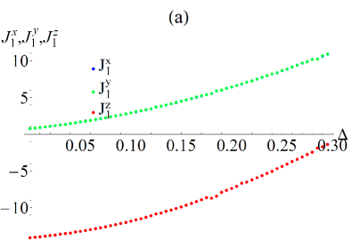
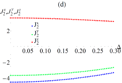
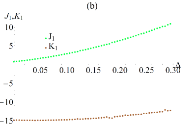
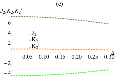
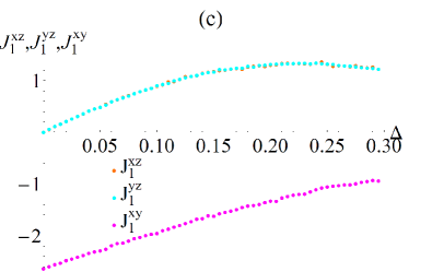
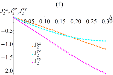
Figure 2: (Colors online) (a) The diagonal exchange couplings $J_{1}^{x},J_{1}^{y},J_{1}^{z}$ and (d) $J_{2}^{x},\,J_{2}^{y},\,J_{2}^{z}$ in meV (shown by blue, green and red lines, respectively); (b) the n. n. Kitaev interaction $K_{1}$ and the n. n. isotropic exchange $J_{1}$ and (e) the second neighbor Kitaev interactions $K_{2}$ and $K_{2}^{\prime}$, as well as the second neighbor isotropic exchange $J_{2}$ in meV (shown by brown, orange and green lines, respectively); (c) the off-diagonal exchange couplings $J_{1}^{xy},\,J_{1}^{xz},\,J_{1}^{yz}$ and (f) $J_{2}^{xy},\,J_{2}^{xz},\,J_{2}^{yz}$ in meV (shown by magenta, orange, cyan lines, respectively) plotted as function of trigonal crystal field $\Delta$ (in eV). The microscopic parameters of the model are considered to be $J_{H}=0.3$ eV, $U_{2}=1.8$ eV, $\lambda=0.4$ eV, $t_{1o}=230$ meV, $t_{d}=67$ meV and $t_{2o}=95$ meV.

IV.2 The second neighbor hopping matrix

Next, we derive the hopping matrix for second neighbors. Six bonds between second neighbors Ir⁴⁺ ions on the honeycomb lattice correspond to (2,1,-1), (1,2,1), (-1,1,2), (-2,-1,1), (-1-2,-1), (1,-1,-2) bonds, which we call ${\tilde{x}}$, ${\tilde{y}}$, ${\tilde{z}}$, and ${\tilde{x}}$, ${\tilde{y}}$, ${\tilde{z}}$ bonds, respectively. Then, the second neighbor ${\tilde{x}}-$bond connects two Ir ions which are also connected by two n. n. Ir-Ir bonds of $y-$ and $z-$ type, and ${\tilde{y}}-$ and ${\tilde{z}}-$bonds connect Ir⁴⁺ ions which are connected by $x-$ and $z-$, and $x-$ and $y-$bonds, respectively. In Fig. 1 (a), we also use the same color coding for the second neighbor bonds as for n. n. bonds: ${\tilde{x}}-$, ${\tilde{y}}-$, ${\tilde{z}}-$ bonds are shown by red, green and blue dotted lines.

Similarly to the hopping between nearest neighbors, there are also two kinds of hoppings connecting second neighbors (see Fig. 1 (a)): the hopping along the path Ir-O-Na-O-Ir, and the direct one. The indirect hopping $t_{2o}$ is large both because it comes from four Ir-O-Na-O-Ir paths but also because it takes advantage of the extended nature of the $s-$orbital of the Na ion. In the ideal structure, it is equal to $t_{2o}=82.1$ meV, and in the presence of the trigonal distortion it is even larger, $t_{2o}=94.7$ meV.katerina13 The direct hopping between second neighbors is significantly smaller than the one between nearest neighbors and also significantly smaller than the hopping along the Ir-O-Na-O-Ir path. In our derivation of the second neighbor super-exchange Hamiltonian, we will neglect all second neighbor hoppings except $t_{2o}$.

Explicitly, the hopping matrix element between second neighbor Ir ions along the ${\tilde{z}}$-bond comes from the following processes:comment

$$\text{Path 1}:\,{\rm Ir}\,(Y)\rightarrow{\rm O}\,(p_{z})\rightarrow{\rm Na}\,(s)\rightarrow{\rm O}\,(p_{z})\rightarrow{\rm Ir}\,(X)$$

$$\text{Path 2}:\,{\rm Ir}\,(Y)\rightarrow{\rm O}\,(p_{z})\rightarrow{\rm Na}\,(s)\rightarrow{\rm O}\,(p_{y})\rightarrow{\rm Ir}\,(X)$$

$$\text{Path 3}:\,{\rm Ir}\,(Y)\rightarrow{\rm O}\,(p_{x})\rightarrow{\rm Na}\,(s)\rightarrow{\rm O}\,(p_{z})\rightarrow{\rm Ir}\,(X)$$

$$\text{Path 4}:\,{\rm Ir}\,(Y)\rightarrow{\rm O}\,(p_{x})\rightarrow{\rm Na}\,(s)\rightarrow{\rm O}\,(p_{y})\rightarrow{\rm Ir}\,(X)$$

Summing over all these four paths, shown by thick magenta lines in Fig. 1 (a), we obtain the effective hopping Hamiltonian between second neighbor Ir⁴⁺ ions along the ${\tilde{z}}$-bond

$$H_{t}^{\tilde{z}}=\sum_{n}\sum_{\gamma,\gamma^{\prime}}T_{2,n,n+{\tilde{z}}}^{\gamma,\gamma^{\prime}}(b_{n,\gamma}^{\dagger}b_{n+{\tilde{z}},\gamma^{\prime}}+h.c.),$$ (47)

where, formally, the hopping matrix $T_{2,n,n+{\tilde{z}}}$ has the same structure as $T_{1,n,n+{z}}$ given by Eq. (46).

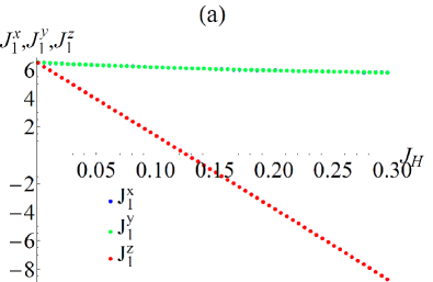
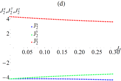
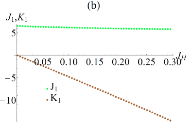
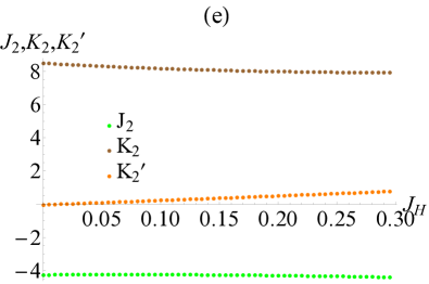
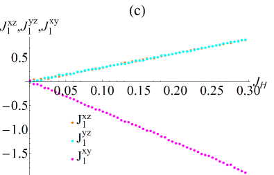
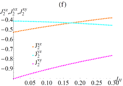
Figure 3: (Colors online) (a) The diagonal exchange couplings $J_{1}^{x},\,J_{1}^{y},\,J_{1}^{z}$ and (d) $J_{2}^{x},\,J_{2}^{y},\,J_{2}^{z}$ in meV (shown by blue, green, red lines, respectively); (b) the n. n. Kitaev interaction $K_{1}$ and the n. n. isotropic exchange $J_{1}$ and (e) the second neighbor Kitaev interactions $K_{2}$ and $K_{2}^{\prime}$, as well as the second neighbor isotropic exchange $J_{2}$ in meV (shown by brown, orange and green lines, respectively); (c) the off-diagonal exchange couplings $J_{1}^{xy},\,J_{1}^{xz},\,J_{1}^{yz}$ and (f) $J_{2}^{xy},\,J_{2}^{xz},\,J_{2}^{yz}$ in meV (shown by magenta, orange, cyan, magenta lines, respectively) plotted as as functions of Hund’s coupling, $J_{H}$ (in eV). The microscopic parameters of the model are considered to be $U_{2}=1.8$ eV, $\lambda=0.4$ eV, $\Delta=0.1$ eV, $t_{1o}=230$ meV, $t_{d}=67$ meV and $t_{2o}=95$ meV.

V The exchange coupling tensors $\Gamma_{1}^{\alpha\beta}$ and $\Gamma_{2}^{\alpha\beta}$

We show in Fig. 2 and Fig. 3 how the matrix elements of the exchange coupling tensor $\Gamma^{\alpha\beta}$, defined in Eq.(42), computed for both nearest and second neighbor Ir⁴⁺ ions depend on the microscopic parameters (trigonal distortion, Hund’s coupling, Coulomb interaction and SO coupling). We note right away that the main role of the Coulomb repulsion is to determine the overall energy scale for the couplings. Thus, in all computations we take, for definitiveness, $U_{2}=1.8$ eV, which is laying inside the range of values, 1.5 eV-2.5 eV, characteristic to iridates. We also set the SO coupling constant to $\lambda=0.4$ eV since it is the value associated with Ir⁴⁺ ions in the literature. As we already mentioned before, we compute all exchange interactions for either $z$-nearest or for ${\tilde{z}}$ next n. n. bonds. Interactions for other bonds can be obtained using symmetry arguments.

V.1 Effect of trigonal distortion.

Here we study the dependencies of the exchange couplings on the trigonal distortion, $\Delta$. At ambient pressure, the trigonal crystal field splitting in both Na₂IrO₃ and Li₂IrO₃ is about 110 meV.gret13 However, it is also believed that a much stronger trigonal distortion can be reached under pressure. In this subsection, the exchange parameters were computed for a fixed Hund’s coupling, $J_{H}=0.3$ eV.

In Fig. 2 (a)-(c), we plot the $\Delta$-dependencies of the matrix elements of the tensor $\Gamma_{1}^{\alpha\beta}$ on the $z$-bond. In order to define n. n. Kitaev interactions on $x$- and $y$-bonds, one needs to permute indices of bonds and couplings which is done with the help of Fig. 4. The diagonal matrix elements $J_{1}^{x},\,J_{1}^{y},\,J_{1}^{z}$ are shown in Fig. 2 (a). We see that while the $J_{1}^{x}$ and $J_{1}^{y}$ couplings are positive and degenerate for all values of the trigonal splitting, $J_{1}^{x}=J_{1}^{y}=J_{1}$, the $J_{1}^{z}$ coupling is first negative but then changes sign at $\Delta\simeq 0.2$ eV. The anisotropic n. n. Kitaev interaction, $K_{1}$, may be defined as the difference between diagonal elements. On the $z$-bond, it is simply given by $K_{1}\equiv J_{1}^{z}-J_{1}$. We plot $J_{1}$ and $K_{1}$ in Fig. 2 (b). Notice that while the n. n. isotropic exchange is antiferromagnetic and is rapidly growing with $\Delta$, the Kitaev interaction is ferromagnetic and is almost independent of the magnitude of the trigonal field.

In Fig. 2 (d)-(f), we plot the $\Delta$-dependencies of the matrix elements of the tensor $\Gamma_{2}^{\alpha\beta}$. We see that the second neighbor diagonal elements $J_{2}^{x},\,J_{2}^{y},\,J_{2}^{z}$, presented in Fig. 2 (d), are substantially weaker than the n. n. diagonal interactions (see Fig. 2 (a)). There is also no degeneracy between them: all of the second neighbor diagonal elements are different from each other except $J_{2}^{z}=-J_{2}^{y}$. If we define the isotropic exchange as $J_{2}^{y}=J_{2}$, and anisotropic second neighbor Kitaev interactions as $K_{2}\equiv J^{z}_{2}-J^{y}_{2}=-2J_{2}$ and $K_{2}^{\prime}\equiv J^{y}_{2}-J^{x}_{2}$, then the interaction on the ${\tilde{z}}$-bond can be written as $J_{2}{\mathbf{S}}{\mathbf{S}}+K_{2}S^{z}S^{z}-K_{2}^{\prime}S^{x}S^{x}$. We plot $J_{2},\,K_{2}$ and $K_{2}^{\prime}$ as a function of $\Delta$ in Fig. 2 (e). Note that for all values of $\Delta$ $J_{2}<0$, $K_{2}>0$ and $K_{2}^{\prime}>0$, and also $K_{2}\gg K_{2}^{\prime}$.

It is also important to remember that $J_{2}$, $K_{2}$ and $K_{2}^{\prime}$ all come from the same process and are governed by the same hopping parameter $t_{2o}$. This is in the contrast to the n. n. couplings, $J_{1}$ and $K_{1}$, for which the super-exchange processes in the absence of the trigonal distortion are completely distinct. $J_{1}$ is determined by the direct hopping, with amplitude $t_{d}$, and $K_{1}$ is determined with amplitude $t_{1o}$, mediated by the hopping through the intermediate oxygen. The interactions between second neighbors come from the same process and are governed by the same hopping parameter $t_{2o}$.

The behavior of the off-diagonal terms $J_{1}^{xy},\,J_{1}^{xz},\,J_{1}^{yz}$ and $J_{2}^{xy},\,J_{2}^{xz},\,J_{2}^{yz}$ is shown in Fig. 2 (c) and (f), respectively. At $\Delta=0$, all of them, except $J_{1}^{xy}$, are equal to zero. The non-zero value of $J_{1}^{xy}$ is due to the finite value of the Hund’s coupling. As we will see in the next subsection, $J_{1}^{xy}(J_{H}=0)=0$. The magnitudes of all off-diagonal terms grow with the strength of the trigonal distortion, however they remain subdominant interactions even at relatively large $\Delta$.

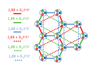
Figure 4: (Colors online) Schematic representation of the effective super-exchange model for Na₂IrO₃. Color coding is the same as in Fig. 1 (a). $X$, $Y$ and $Z$ $t_{2g}$ electronic orbitals, participating in the super-exchange, are shown by red, green and blue small circles.

V.2 Effect of Hund’s coupling.

In Fig. 3, we present the dependence of the exchange couplings on the Hund’s interaction, $J_{H}$. Here we fix the trigonal distortion equal to $\Delta=0.1$ eV.

In Fig. 3 (a) and (d), we plot $J_{1}^{x},\,J_{1}^{y},\,J_{1}^{z}$ and $J_{2}^{x},\,J_{2}^{y},\,J_{2}^{z}$, respectively. At $J_{H}=0$, we see that the n. n. diagonal couplings are all equal, $J_{1}^{x}=J_{1}^{y}=J_{1}^{z}$. Consequently, the n. n. Kitaev interaction is $K_{1}=0$. The n. n. off-diagonal couplings (see Fig. 3 (c)) are also zero at $J_{H}=0$. On the contrary, the next n. n. diagonal couplings are only partially degenerate: $J_{2}^{x}=J_{2}^{y}=-J_{2}^{z}$. Thus, $K_{2}\neq 0$ and $K_{2}^{\prime}\neq 0$. The second neighbor off-diagonal couplings (see Fig. 3 (f)) are all non-zero but very small. Thus, at $J_{H}=0$ the leading anisotropic term is the Kitaev interaction between second neighbors, $K_{2}$. With increasing $J_{H}$, the n. n. Kitaev interaction, $K_{1}$, rapidly grows and, at realistic values of Hund’s coupling, about 0.2-0.3 eV, becomes the dominant interaction. With increasing $J_{H}$, $K_{1}$ rapidly grows and becomes the dominant interaction at realistic values of Hund’s coupling, about 0.2-0.3 eV. The other exchange couplings also change with $J_{H}$. Overall, the n. n. interactions are more sensitive to the strength of the Hund’s coupling than the second neighbors.

Let us summarize the results obtained in this section. The most important anisotropies resulting from our microscopic calculations are the Kitaev interactions on n. n. and next n. n. bonds, $K_{1}$ and $K_{2}$ respectively. All other anisotropic interactions remain subdominant for reasonable values of miscroscopic parameters. $K_{1}$ is weakly dependent on the trigonal CF, but grows quickly with Hund’s coupling. However, $K_{2}$ depends weakly on both $\Delta$ and $J_{H}$.

VI Magnetic phase diagram

VI.1 Effective super-exchange model for Na₂IrO₃.

We now discuss how the above results apply to the case of Na₂IrO₃. We take the values of the microscopic parameters most closely related to Na₂IrO₃: $\lambda=0.4$ eV, $\Delta=0.1$ eV, $J_{H}=0.3$ eV, $U_{2}=1.8$ eV, and hopping matrix elements equal to $t_{1o}=230$ meV, $t_{d}=67$ meV and $t_{2o}=95$ meV.katerina13 We obtain the following exchange couplings: $J_{1}=5.8$ meV, $K_{1}=-14.8$ meV, $J_{2}=-4.4$ meV, $K_{2}=7.9$ meV. Calculated n. n. exchange constants are in fair agreement with the results of ab-initio quantum chemistry calculations by Katukuri et al:katukuri14 $J_{1}\simeq 3$ meV and $K_{1}\simeq-17.5$ meV.

Our results for n. n. couplings confirm the previous conclusionsingh10 ; singh12 ; liu11 ; ye12 ; choi12 that the super-exchange model with only n. n. couplings is insufficient to explain the experimentally observed zigzag magnetic order even in the presence of the trigonal distortion. Recall that in the original Kitaev-Heisenberg model,jackeli09 ; jackeli10 the isotropic and Kitaev exchange couplings were parameterized by a single parameter $\alpha$ as $J_{1}=1-\alpha$ and $K_{1}=2\alpha$. Taking $J_{1}$ and $K_{1}$ obtained for the trigonal distortion $\Delta\simeq$0.1 eV, we get $\alpha\simeq 0.57$, which corresponds to the stripy antiferromagnetic order instead of the zigzag-type order. Neglecting the trigonal distortion and taking $J_{1}=1.4$ meV and $K_{1}=-15.2$ meV obtained at $\Delta=$0 eV, we get $\alpha\simeq 0.83$ corresponding to the spin liquid, which was desired but not observed in Na₂IrO₃.singh10 ; singh12 ; liu11 ; ye12 ; choi12

This shows that, in addition to the antiferromagnetic Heisenberg and ferromagnetic Kitaev n.n. interactions, the minimal model has to include further neighbor interactions. As we saw in Sec.V, the dominant microscopic Ir-Ir couplings also include next n. n. ferromagnetic Heisenberg and antiferromagnetic Kitaev interactions, which also must be considered.

Thus, let us study the following super-exchange Hamiltonian:

$$\mathcal{H}=J_{1}\sum_{\langle n,n^{\prime}\rangle_{\gamma}}{\bf S}_{n}{\bf S}_{n^{\prime}}+K_{1}\sum_{\langle n,n^{\prime}\rangle_{\gamma}}S_{n}^{\gamma}S_{n^{\prime}}^{\gamma}$$

$$+J_{2}\sum_{\langle\langle n,n^{\prime}\rangle\rangle_{\tilde{\gamma}}}{\bf S}_{n}{\bf S}_{n^{\prime}}+K_{2}\sum_{\langle\langle n,n^{\prime}\rangle\rangle_{\tilde{\gamma}}}S_{n}^{\gamma}S_{n^{\prime}}^{\tilde{\gamma}}$$ (48)

$$+J_{3}\sum_{\langle\langle\langle n,n^{\prime}\rangle\rangle\rangle}{\bf S}_{n}{\bf S}_{n^{\prime}},$$

where $J_{1}>0$, $K_{1}<0$, $J_{2}<0$, $K_{2}=-2J_{2}>0$, and $J_{3}>0$. Note that in our formulation of the minimal model (48), we also include the third neighbor antiferromagnetic coupling, which was suggested to be crucial for stabilizing the zigzag magnetic order in the previous works.kimchi11 ; choi12

It is very important that the presence of the second n. n. Kitaev interaction does not change the space group symmetries of the effective model: the model (48) has the same symmetries as the original Kitaev-Heisenberg model. The schematic representation of the n.n. and second n. n. interactions is shown in Fig. 4. As in Fig. 1 (a), the solid lines correspond to n. n. bonds and dotted lines correspond to the second n. n. Kitaev interaction. We also note that the same form of the second neighbor interactions was previously obtainedrachel10 ; reuther12 in the limit $U\rightarrow\infty$ of the Kane-Mele-Hubbard model.kane05

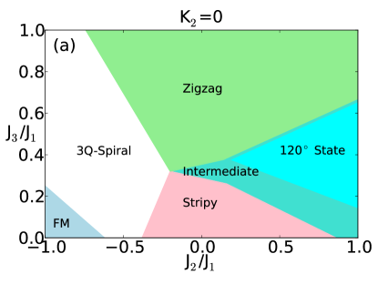
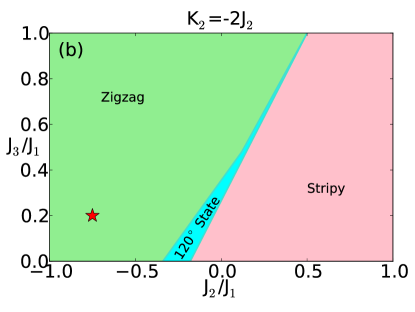
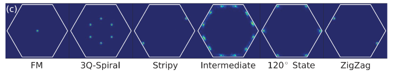
Figure 5: (Colors online) Phase diagrams of the effective model (48) obtained with the classical Monte Carlo simulations at low temperature $T=0.1J_{1}$ for (a) second neighbor Kitaev interaction equal to $K_{2}=0$, (b) second neighbor Kitaev interaction $K_{2}=-2J_{2}$. The simulation is done for $J_{1}=3$ meV and $K_{1}=-17$ meV. The blue, rose, green, white, cyan and emerald regions show the ferromagnetic (FM), the stripy, the zigzag, the incommensurate $3{\mathbf{Q}}-$spiral, the 120^∘ structure and the intermediate state, respectively. The red star is placed in the region which might well characterize the set of interactions for Na₂IrO₃. (c) The structure factors obtained as a Fourier transform of a snapshot of a given configuration for each of these magnetic phases. Sharp peaks appear at the corresponding ordering wavevector.

VI.2 The magnetic phase diagram

We computed the phase diagram of the effective model (48) with classical Monte Carlo simulations based on the standard Metropolis algorithm. To explore the physics of the model (48), we fix n. n. interactions to $J_{1}=3$ meV and $K_{1}=-17$ meV values, which were obtained by quantum chemistry calculations by Katukuri et alkatukuri14 and are within the range of parameters obtained by us in this paper. We compute the phase diagram not only for ferromagnetic, $J_{2}<0$, but also for antiferromagnetic, $J_{2}>0$, second neighbor interaction. This allows us to compare our findings with other phase diagrams that were previously obtained in the literature.kimchi11 ; katukuri14 The simulations were performed at low temperature $T=0.1J_{1}$, at which for the full range of the considered parameters the model is in the magnetically ordered state.

The phase diagram of the model (48) in the limit of zero second neighbor Kitaev interaction, $K_{2}=0$, is presented in Fig. 5 (a). A more realistic phase diagram computed with $K_{2}=-2J_{2}$ is presented in Fig. 5 (b). Even at first glance, we see that the second n. n. Kitaev interaction suppresses the ferromagnetic and spiral phases and stabilizes the antiferromagnetic zigzag and stripy phases.

In order to get a better sense of the basic structure of the different states composing the phase diagrams, we also performed a numerical Fourier transform of a snapshot of the ground state spin configuration at a given point of the phase diagram. From that Fourier transform, we computed the corresponding spin structure factor, which allows us to determine the dominant wavevectors of that configuration. We plot the spin structure factors in Fig. 5 (c).

VI.2.1 Phase diagram of the $J_{1}-J_{2}-J_{3}-K_{1}-0$ model (Fig.5 (a)).

The $K_{2}=0$ phase diagram is very rich, but overall it is qualitatively similar to both the classical phase diagram of the $J_{1}-J_{2}-J_{3}-K_{1}$kimchi11 ; katukuri14 and of the pure Heisenberg $J_{1}-J_{2}-J_{3}$ model on the honeycomb lattice.choi12 It displays the ferromagnetic (blue region), the stripy (rose region) and the zigzag antiferromagnetic states (green region), the $3{\mathbf{Q}}-$incommensurate spiral state (white region), the 120^∘ order (cyan region) and a very particular multi-${\mathbf{Q}}$ incommensurate state (dark cyan region), which we call an ”intermediate” phase, as it always separates the 120^∘ order from either the stripy or the zigzag phases. The Néel antiferromagnetic order is also one of the possible ground states of the model. However, the n. n. Kitaev term, $K_{1}$, and the second neighbor Heisenberg term, $J_{2}$, destabilize it in favor of the stripy and zigzag phases. The Néel order is realized only at values of $J_{3}/J_{1}>1$, which are not shown in the Fig. 5 (a).

The simplest state we find on the phase diagram is the ferromagnetic state which is characterized by a single ${\mathbf{Q}}=(0,0)$ wavevector. This state is the ground state in the region of large ferromagnetic $J_{2}$ and small $J_{3}$ couplings. As $J_{2}$ is decreased and $J_{3}$ is increased, the ferromagnetic state becomes unstable with respect to a spiral state, which is built out of three incommensurate wavevectors related by $C_{3}$ rotation. Because the ordering ${\mathbf{Q}}$ vectors are not connected by reciprocal lattice vectors, the spiral phase represents an example of a $3{\mathbf{Q}}-$incommensurate order. Note that the magnitude of the ordering wavevector $|{\mathbf{Q}}|$ varies throughout the phase.

The stripy and zigzag antiferromagnetic orders are found for both ferromagnetic and antiferromagnetic $J_{2}$ interaction of intermediate strength. However, while the stripy order is found at small values of the third n. n. interaction, $J_{3}$, the experimentally observed zigzag order is found only at values $J_{3}\geq 0.35J_{1}$ which seem too large given that tight-binding hopping amplitudes are clearly dominated by the n. n. and the second neighbor terms.katerina13 Both the stripy and the zigzag phases are single-${\mathbf{Q}}$ orders, characterized by one of the symmetry related wavevectors: ${\mathbf{Q}}_{1}=(0,\frac{2\pi}{3})$, ${\mathbf{Q}}_{2}=(\frac{\pi}{3},\frac{\pi}{\sqrt{3}})$ and ${\mathbf{Q}}_{3}=(-\frac{\pi}{3},\frac{\pi}{\sqrt{3}})$.

The stripy and the zigzag phases are separated by a 120^∘ state characterized by one of the ${\mathbf{Q}}_{1}=(\frac{4\pi}{3\sqrt{3}},0)$, ${\mathbf{Q}}_{2}=(\frac{2\pi}{3\sqrt{3}},\frac{2\pi}{3})$ and ${\mathbf{Q}}_{3}=(-\frac{2\pi}{3\sqrt{3}},\frac{2\pi}{3})$ wavevectors. Because these vectors are connected by the reciprocal lattice vectors, this is a coplanar single-${\mathbf{Q}}$ spiral which describes the 120^∘ spin ordering within each of the two sublattices forming the honeycomb lattice. As $x$, $y$ and $z$ components of spins are all equally modulated in this 120^∘ state, the spins in this state are lying in one of the (111) planes.

The transition from the stripy and the zigzag states into the 120^∘ state is not direct; it happens through the intermediate phase. This transition can be understood by looking at the evolution of the spin structure factors. We find that before the onset of the 120^∘ state the transition from a single-${\mathbf{Q}}$ stripy (or a single-${\mathbf{Q}}$ zigzag) state to a state defined by a superposition of three different stripy (zigzag) phases. The structure factor for this state is characterized by the presence of six peaks situated in the middle of the edges of the first BZ hexagon. These peaks split into two incommensurate peaks with ${\mathbf{Q}}$ vectors sliding along the edges (see Fig. 5 (c) for the structure factor corresponding to the Intermediate phase) until they reach wavevectors at the hexagon’s corners characterizing the 120^∘ structure. Here, we note that this 120^∘ state separating the stripy and the zigzag phases was also obtained by Rau et alrau14 as a classical ground state of the n. n. super-exchange in the presence of the symmetric off-diagonal exchange.

Here a comment is in order. In each of the stripy and the zigzag phases obtained in the Kitaev-Heisenberg models without further neighbor interactions,jackeli10 ; jackeli13 ; price12 ; price13 the spins were aligned along one of the cubic directions. The spin direction was locked to the spatial orientation of a stripy or a zigzag pattern defined by the wavector ${\mathbf{Q}}$. Both the locking of the spin direction and the way the translational symmetry is broken, i.e. the choice of ${\mathbf{Q}}$, are defined on the classical level.

In the absence of $J_{2}$ and $J_{3}$ interactions, the stripy phase is stabilized only for the ferromagnetic n. n. Kitaev interaction, $K_{1}<0$, and the zigzag phase is stabilized only for the antiferromagnetic n. n. Kitaev interaction, $K_{1}>0$. Consider the stripy order with ferromagnetic $z$-bonds. In this state, the spins and, therefore, the order parameter are pointing along $z$ cubic axis. This state has the lowest classical energy, because such a direction of the order parameter maximizes the energy gain due to the ferromagnetic Kitaev interaction on ferromagnetic $z$-bonds. The same reasoning explains why the spins in $x$ and $y$ stripes are pointing along the $x$ and $y$ axes respectively.

Next, consider the zigzag order characterized by ferromagnetic $x-$ and $y-$bonds. In this state, the spins also point along the $z$ cubic axis because it maximizes the energy gain due to the antiferromagnetic Kitaev interaction on the antiferromagnetic $z-$ bonds.

In the presence of further neighbor couplings the situation is different. As we can see in Fig. 5 (a), both the stripy and the zigzag order can be stabilized for the ferromagnetic n. n. Kitaev interaction. While the situation for the stripy phase is the same as before, where the spins point along the cubic direction corresponding to the label of the ferromagnetic bond to gain energy from the ferromagnetic Kitaev interaction, the direction of the zigzag order parameter is not defined on the classical level. Instead, there are two ferromagnetic bonds in the zigzag phase, e.g. $x$ and $y$. Thus, all zigzag states characterized by an order parameter pointing along any direction in the $xy$-plane are classically degenerate. The direction of the order parameter is then selected by order from disorder mechanism, in which spin fluctuations (quantum or thermal) remove the accidental degeneracy and select the true ordered state. We have checked with Monte Carlo simulations that thermal fluctuations again choose the states in which spins point along either $x$ or $y$ cubic directions. The full finite-temperature phase diagram for the model (48) will be published elsewhere.

VI.2.2 Phase diagram of the $J_{1}-J_{2}-J_{3}-K_{1}-K_{2}$ model (Fig. 5 (b)).

In Fig. 5 (b), we present the magnetic phase diagram of the model (48) when the second neighbor Kitaev interaction is equal to $K_{2}=-2J_{2}$, as predicted by our theory when the second neighbors are coupled only through the Ir-O-Na-O-Ir superexchange path. We see that the phase diagram greatly simplifies. The second neighbor Kitaev term suppresses the spiral and the ferromagnetic phases in favor of the stripy and zigzag order which now dominate for antiferromagnetic and ferromagnetic $J_{2}$, respectively. These two phases are still separated by the 120^∘ order and Intermediate phase, but both the 120^∘ phase and, especially, the Intermediate phase shrink significantly. However, the most important effect of the second neighbor Kitaev term is that for sufficient ferromagnetic $J_{2}<0$, it stabilizes the zigzag even for $J_{3}=0$. In Fig. 5 (b), we put the red star next to the point which might well characterize the set of interactions for Na₂IrO₃.

It is worth noting that addition of non-zero $K_{2}$ interaction also does not determine the direction of zigzag order parameter on the classical level. For the zigzag order with antiferromagnetic $z$-bonds discussed above, all states with spins lying in the $xy$-plane remain classically degenerate. This can be understood as follows. In the zigzag order with antiferromagnetic $z$-bonds, the second n. n. ${\tilde{z}}$-bonds are ferromagnetic while the ${\tilde{x}}$- and ${\tilde{y}}$-bonds are antiferromagnetic. Thus, the antiferromagnetic $K_{2}$ coupling on these bonds will keep the spins in the $xy$-plane. However, since there is an equal number of ${\tilde{x}}$- and ${\tilde{y}}$-bonds, the $K_{2}$ interaction does not lift the classical degeneracy. A particular spin direction, $x$ or $y$, is again chosen by fluctuations.

VII Conclusions

To summarize, two avenues were explored in this work. First, we performed the derivation of an effective super-exchange Hamiltonian that governs the magnetic properties of the honeycomb iridates treating the many-body and single electron interactions on an equal footing. We demonstrated that in the presence of strong SO coupling, this effective Hamiltonian forms a symmetric second-rank tensor with non-equivalent diagonal and non-zero off-diagonal elements. We performed a detailed analysis of the magnetic interactions as a function of the Hund’s coupling representing the electronic correlations and the trigonal CF splitting which governs the single-electron physics. We showed that the main role of the Hund’s coupling is that it is responsible for the appearance of the Kitaev anisotropic interactions via the non-equivalence of the diagonal elements. The trigonal CF also affects the diagonal interactions, however, it’s dominating role is in controlling the strength of the off-diagonal interactions. While these interactions might be significantly increased by external pressure, at ambient pressure the trigonal CF distortion is small and, consequently, the off-diagonal interactions are subdominant. Thus, we neglected off-diagonal terms in the derivation of the super-exchange model (48), which we believe is the minimal model to describe the Na₂IrO₃ compound. This model includes five Ir-Ir couplings: n. n. antiferromagnetic Heisenberg and ferromagnetic Kitaev interactions, next n. n. ferromagnetic Heisenberg and antiferromagnetic Kitaev interactions, and third n. n. antiferromagnetic Heisenberg interaction.

The study of the classical phase diagram for this minimal model constitutes the second part of the paper. We computed the low temperature phase diagram of the effective model (48) with classical Monte Carlo simulations. Due to the presence of the anisotropic Kitaev interactions and the frustration introduced by the competition of the spin couplings between n. n. and second neighbors, the resulting phase diagram is very rich. It contains both various commensurate states and incommensurate single-${\mathbf{Q}}$ and multi-${\mathbf{Q}}$ phases, whose regions of stability are controlled by the ratios between competing exchange constants. We showed that the second neighbor Kitaev term plays an important role in the stabilization of the commensurate antiferromagnetic zigzag phase which has been experimentally observed in Na₂IrO₃. In our simulations, we found this phase to be the ground state for parameters of the model of both the correct signs and magnitudes.

Acknowledgements. We thank Katerina Foyevtsova, Michel Gingras, George Jackeli and Arun Paramekanti for useful discussions. This work was supported, in part, by the National Science Foundation under Grant No. PHYS-1066293 and the hospitality of the Aspen Center for Physics. N.P. and Y.S. acknowledge the support from NSF grant DMR-1255544. P.W. thanks the Department of Physics at the University of Wisconsin-Madison for hospitality during a stay as a visiting professor. P.W. also acknowledges partial support through the DFG research unit ”Quantum phase transitions”.

Appendix A The structure of the exchange coupling tensor $\Gamma^{\alpha\beta}$

The elements of the exchange coupling tensor $\Gamma^{\alpha\beta}$ are given by the following expressions:

$$J_{x}=-\sum_{\xi}\frac{1}{\epsilon_{\xi}} \Bigl{(}A_{\uparrow\uparrow}^{\xi}\left(A_{\downarrow\downarrow}^{\xi}\right)^{*}+A_{\downarrow\downarrow}^{\xi}\left(A_{\uparrow\uparrow}^{\xi}\right)^{*}$$

$$+A_{\uparrow\downarrow}^{\xi}\left(A_{\downarrow\uparrow}^{\xi}\right)^{*}+A_{\downarrow\uparrow}^{\xi}\left(A_{\uparrow\downarrow}^{\xi}\right)^{*}\Bigr{)},$$

$$J_{y}=\sum_{\xi}\frac{1}{\epsilon_{\xi}} \Bigl{(}A_{\uparrow\uparrow}^{\xi}\left(A_{\downarrow\downarrow}^{\xi}\right)^{*}+A_{\downarrow\downarrow}^{\xi}\left(A_{\uparrow\uparrow}^{\xi}\right)^{*}$$

$$-A_{\uparrow\downarrow}^{\xi}\left(A_{\downarrow\uparrow}^{\xi}\right)^{*}-A_{\downarrow\uparrow}^{\xi}\left(A_{\uparrow\downarrow}^{\xi}\right)^{*}\Bigr{)},$$

$$J_{z}=-\sum_{\xi}\frac{1}{\epsilon_{\xi}} \Bigl{(}A_{\uparrow\uparrow}^{\xi}\left(A_{\uparrow\uparrow}^{\xi}\right)^{*}+A_{\downarrow\downarrow}^{\xi}\left(A_{\downarrow\downarrow}^{\xi}\right)^{*}$$

$$-A_{\uparrow\downarrow}^{\xi}\left(A_{\uparrow\downarrow}^{\xi}\right)^{*}-A_{\downarrow\uparrow}^{\xi}\left(A_{\downarrow\uparrow}^{\xi}\right)^{*}\Bigr{)},$$

$$J_{z}=-\sum_{\xi}\frac{1}{\epsilon_{\xi}} \Bigl{(}A_{\uparrow\uparrow}^{\xi}\left(A_{\uparrow\uparrow}^{\xi}\right)^{*}+A_{\downarrow\downarrow}^{\xi}\left(A_{\downarrow\downarrow}^{\xi}\right)^{*}$$

$$-A_{\uparrow\downarrow}^{\xi}\left(A_{\uparrow\downarrow}^{\xi}\right)^{*}-A_{\downarrow\uparrow}^{\xi}\left(A_{\downarrow\uparrow}^{\xi}\right)^{*}\Bigr{)},$$

$$J_{xy}=\imath\sum_{\xi}\frac{1}{\epsilon_{\xi}} \Bigl{(}A_{\uparrow\uparrow}^{\xi}\left(A_{\downarrow\downarrow}^{\xi}\right)^{*}-A_{\downarrow\downarrow}^{\xi}\left(A_{\uparrow\uparrow}^{\xi}\right)^{*}$$

$$+A_{\downarrow\uparrow}^{\xi}\left(A_{\uparrow\downarrow}^{\xi}\right)^{*}-A_{\uparrow\downarrow}^{\xi}\left(A_{\downarrow\uparrow}^{\xi}\right)^{*}\Bigr{)},$$

$$J_{yx}=\imath\sum_{\xi}\frac{1}{\epsilon_{\xi}} \Bigl{(}A_{\uparrow\uparrow}^{\xi}\left(A_{\downarrow\downarrow}^{\xi}\right)^{*}-A_{\downarrow\downarrow}^{\xi}\left(A_{\uparrow\uparrow}^{\xi}\right)^{*}$$

$$-A_{\downarrow\uparrow}^{\xi}\left(A_{\uparrow\downarrow}^{\xi}\right)^{*}+A_{\uparrow\downarrow}^{\xi}\left(A_{\downarrow\uparrow}^{\xi}\right)^{*}\Bigr{)},$$

$$J_{xz}=\sum_{\xi}\frac{1}{\epsilon_{\xi}} \Bigl{(}A_{\uparrow\uparrow}^{\xi}\left(A_{\downarrow\uparrow}^{\xi}\right)^{*}-A_{\downarrow\downarrow}^{\xi}\left(A_{\uparrow\downarrow}^{\xi}\right)^{*}$$

$$+A_{\downarrow\uparrow}^{\xi}\left(A_{\uparrow\uparrow}^{\xi}\right)^{*}-A_{\uparrow\downarrow}^{\xi}\left(A_{\downarrow\downarrow}^{\xi}\right)^{*}\Bigr{)},$$

$$J_{zx}=\sum_{\xi}\frac{1}{\epsilon_{\xi}} \Bigl{(}A_{\uparrow\uparrow}^{\xi}\left(A_{\uparrow\downarrow}^{\xi}\right)^{*}-A_{\downarrow\downarrow}^{\xi}\left(A_{\downarrow\uparrow}^{\xi}\right)^{*}$$

$$+A_{\uparrow\downarrow}^{\xi}\left(A_{\uparrow\uparrow}^{\xi}\right)^{*}-A_{\downarrow\uparrow}^{\xi}\left(A_{\downarrow\downarrow}^{\xi}\right)^{*}\Bigr{)},$$

$$J_{yz}=\imath\sum_{\xi}\frac{1}{\epsilon_{\xi}} \Bigl{(}A_{\uparrow\uparrow}^{\xi}\left(A_{\downarrow\uparrow}^{\xi}\right)^{*}+A_{\downarrow\downarrow}^{\xi}\left(A_{\uparrow\downarrow}^{\xi}\right)^{*}$$

$$-A_{\uparrow\downarrow}^{\xi}\left(A_{\downarrow\downarrow}^{\xi}\right)^{*}-A_{\downarrow\uparrow}^{\xi}\left(A_{\uparrow\uparrow}^{\xi}\right)^{*}\Bigr{)},$$

$$J_{zy}=\imath\sum_{\xi}\frac{1}{\epsilon_{\xi}} \Bigl{(}A_{\uparrow\uparrow}^{\xi}\left(A_{\uparrow\downarrow}^{\xi}\right)^{*}+A_{\downarrow\downarrow}^{\xi}\left(A_{\downarrow\uparrow}^{\xi}\right)^{*}$$

$$-A_{\uparrow\downarrow}^{\xi}\left(A_{\uparrow\uparrow}^{\xi}\right)^{*}-A_{\downarrow\uparrow}^{\xi}\left(A_{\downarrow\downarrow}^{\xi}\right)^{*}\Bigr{)},$$

Here, in order to shorten notations, we omitted the site indices denoting $A_{n,n^{\prime};\sigma,\sigma^{\prime}}^{\xi}\equiv A_{\sigma,\sigma^{\prime}}^{\xi}$ and $A_{n^{\prime},n;\sigma^{\prime},\sigma}^{\xi}\equiv\left(A_{\sigma,\sigma^{\prime}}^{\xi}\right)^{*}$.

References

- (1) N. B. Perkins, Y. Sizyuk and P. Wölfle, Phys. Rev. B 89, 035143 (2014).
- (2) G. Jackeli and G. Khaliullin, Phys. Rev. Lett. 102, 017205 (2009).
- (3) I. E. Dzyaloshinskii, J. Phys. Chem. Solids 4, 241 (1958).
- (4) T. Moriya, Phys. Rev. Lett. 4, 228 (1960).
- (5) A. Kitaev, Ann. Phys. 321, 2 (2006).
- (6) J. Chaloupka, G. Jackeli, and G. Khaliullin, Phys. Rev. Lett. 105, 027204 (2010).
- (7) G. Cao, J. Bolivar, S. McCall, J.E. Crow, and R.P. Guertin, Phys. Rev. B 57, R11039 (1998).
- (8) B. J. Kim, Hosub Jin, S. J. Moon, J.-Y. Kim, B.-G. Park, C. S. Leem, Jaejun Yu, T. W. Noh, C. Kim, S.-J. Oh, J.-H. Park, V. Durairaj, G. Cao, and E. Rotenberg Phys. Rev. Lett. 101, 076402 (2008).
- (9) S. J. Moon, Hosub Jin, W. S. Choi, J. S. Lee, S. S. A. Seo, J. Yu, G. Cao, T. W. Noh, and Y. S. Lee Phys. Rev. B 80, 195110 (2009).
- (10) B. J. Kim, H. Ohsumi, T. Komesu, S. Sakai, T. Morita, H. Takagi and T. Arima, Science 323, 1329 (2009).
- (11) R. Comin, G. Levy, B. Ludbrook, Z.-H. Zhu, C. N. Veenstra, J. A. Rosen, Yogesh Singh, P. Gegenwart, D. Stricker, J. N. Hancock, D. van der Marel, I. S. Elfimov, and A. Damascelli, Phys. Rev. Lett. 109, 266406 (2012)
- (12) S. Fujiyama, H. Ohsumi, K. Ohashi, D. Hirai, B.J. Kim, T. Arima, M. Takata, H. Takagi, Phys. Rev. Lett. 112, 016405 (2014).
- (13) Y. Singh and P. Gegenwart, Phys. Rev. B 82, 064412 (2010).
- (14) Y. Singh, S. Manni, J. Reuther, T. Berlijn, R. Thomale, W. Ku, S. Trebst, and P. Gegenwart, Phys. Rev. Lett. 108, 127203 (2012).
- (15) X. Liu, T. Berlijn, W.-G. Yin, W. Ku, A. Tsvelik, Young-June Kim, H. Gretarsson, Y. Singh, P. Gegenwart, and J. P. Hill, Phys. Rev. B 83, 220403 (2011).
- (16) F. Ye, S. Chi, H. Cao, B. C. Chakoumakos, J. A. Fernandez-Baca, R. Custelcean, T. F. Qi, O. B. Korneta, and G. Cao, Phys. Rev. B 85, 180403 (2012).
- (17) S. K. Choi, R. Coldea, A. N. Kolmogorov, T. Lancaster, I. I. Mazin, S. J. Blundell, P. G. Radaelli, Yogesh Singh, P. Gegenwart, K. R. Choi, S.-W. Cheong, P. J. Baker, C. Stock, and J. Taylor, Phys. Rev. Lett. 108, 127204 (2012).
- (18) Craig C. Price and Natalia B. Perkins, Phys. Rev. Lett. 109, 187201 (2012).
- (19) Craig C. Price and Natalia B. Perkins, Phys. Rev. B 88, 024410 (2013).
- (20) Subhro Bhattacharjee, Sung-Sik Lee, Yong Baek Kim, New J. Phys. 14, 073015 (2012).
- (21) Kateryna Foyevtsova, Harald O. Jeschke, I. I. Mazin, D. I. Khomskii, and Roser Valentí Phys. Rev. B 88, 035107 (2013).
- (22) I. Kimchi and Y.Z. You, Phys. Rev. B 84, 180407(R) (2011).
- (23) J. Chaloupka, G. Jackeli, G. Khaliullin, Phys. Rev. Lett. 110, 097204 (2013).
- (24) Vamshi M. Katukuri, S. Nishimoto, V. Yushankhai, A. Stoyanova, H. Kandpal, Sungkyun Choi, R. Coldea, I. Rousochatzakis, L. Hozoi, Jeroen van den Brink, New J. Phys. 16, 013056 (2014).
- (25) The paths which connect third nearest neighbors are similar to the second neighbors. Starting from the same Ir4+ ions as in the main text, the four dominant paths connecting third neighbors will be , , , . All these paths connect the same orbitals and, thus, contribute mostly to the isotropic Heisenberg exchange. The small anisotropic part is similar in form to the term.
- (26) H. Gretarsson, J. P. Clancy, X. Liu et al, Phys. Rev. Lett. 110, 076402 (2013).
- (27) S. Rachel and K. Le Hur, Phys. Rev. B 82, 075106 (2010).
- (28) J. Reuther, R. Thomale, S. Rachel, Phys. Rev. B 86, 155127 (2012).
- (29) C. L. Kane and E. J. Mele, Phys. Rev. Lett. 95, 146802 (2005); Phys. Rev. Lett. 95, 226801 (2005).
- (30) Jeffrey G. Rau, Eric Kin-Ho Lee, Hae-Young Kee, Phys. Rev. Lett. 112, 077204 (2014).