The impact of gas bulk rotation on the Lyman $\alpha$ line

Abstract

We present results of radiative transfer calculations to measure the impact of gas bulk rotation on the morphology of the Lyman $\alpha$ emission line in distant galaxies. We model a galaxy as a sphere with an homogeneous mixture of dust and hydrogen at a constant temperature. These spheres undergo solid-body rotation with maximum velocities in the range $0-300$  km s^-1and neutral hydrogen optical depths in the range $\tau_{\rm H}=10^{5}-10^{7}$. We consider two types of source distributions in the sphere: central and homogeneous. Our main result is that rotation introduces a dependence of the line morphology with viewing angle and rotational velocity. Observations with a line of sight parallel to the rotation axis yield line morphologies similar to the static case. For lines of sight perpendicular to the rotation axis both the intensity at the line center and the line width increase with rotational velocity. Along the same line of sight, the line becomes single peaked at rotational velocities close to half the line width in the static case. Notably, we find that rotation does not induce any spatial anisotropy in the integrated line flux, the escape fraction or the average number of scatterings. This is because Lyman α scattering through a rotating solid-body proceeds identical as in the static case. The only difference is the doppler shift from the different regions in the sphere that move with respect to the observer. This allows us to derive an analytic approximation for the viewing-angle dependence of the emerging spectrum, as a function of rotational velocity.

1. Introduction

The detection of strong Ly$\alpha$ emission lines has become an essential method in extra-galactic astronomy to find distant star-forming galaxies (Partridge & Peebles, 1967; Rhoads et al., 2000; Gawiser et al., 2007; Koehler et al., 2007; Ouchi et al., 2008; Yamada et al., 2012; Schenker et al., 2012; Finkelstein et al., 2013). The galaxies detected using this method receive the name of Ly$\alpha$ emitters (LAEs). A detailed examination of this galaxy population has diverse implications for galaxy formation, reionization and the large scale structure of the Universe. Attempts to fully exploit the physical information included in the Ly$\alpha$ line require an understanding of all the physical factors involved in shaping the line. Due to the resonant nature of this line, these physical factors notably include temperature, density and bulk velocity field of the neutral Hydrogen in the emitting galaxy and its surroundings.

A basic understanding of the quantitative behavior of the Ly$\alpha$ line has been reached through analytic studies in the case of a static configurations, such as uniform slabs (Adams, 1972; Harrington, 1973; Neufeld, 1990) and uniform spheres (Dijkstra et al., 2006). Analytic studies of configurations including some kind of bulk flow only include the case of a sphere with a Hubble like expansion flow (Loeb & Rybicki, 1999).

A more detailed quantitative description of the Ly$\alpha$ line has been reached through Monte Carlo simulations (Auer, 1968; Avery & House, 1968; Adams, 1972). In the last two decades these studies have become popular due to the availability of computing power. Early into the 21st century, the first studies focused on homogeneous and static media (Ahn et al., 2000, 2001; Zheng & Miralda-Escudé, 2002). Later on, the effects of clumpy media (Hansen & Oh, 2006) and expanding/contracting shell/spherical geometries started to be studied (Ahn et al., 2003; Verhamme et al., 2006; Dijkstra et al., 2006). For a recent review, we refer the interested reader to Dijkstra (2014). Similar codes have applied these results to semi-analytic models of galaxy formation (Orsi et al., 2012; Garel et al., 2012) and results of large hydrodynamic simulations (Forero-Romero et al., 2011, 2012; Behrens & Niemeyer, 2013). Recently, Monte Carlo codes have also been applied to the results of high resolution hydrodynamic simulations of individual galaxies (Laursen et al., 2009; Barnes et al., 2011; Verhamme et al., 2012; Yajima et al., 2012). Meanwhile, recent developments have been focused on the systematic study of clumpy outflows (Dijkstra & Kramer, 2012) and anisotropic velocity configurations (Zheng & Wallace, 2013).

The recent studies of galaxies in hydrodynamic simulations (Laursen et al., 2009; Barnes et al., 2011; Verhamme et al., 2012; Yajima et al., 2012) have all shown systematic variations in the Ly$\alpha$ line with the viewing angle. These variations are a complex superposition of anisotropic density configurations (i.e. edge-on vs. face-on view of a galaxy), the inflows observed by gas cooling and the outflows included in the supernova feedback process of the simulation. These bulk flows physically correspond to the circumgalactic and intergalactic medium (CGM and IGM). These effects are starting to be studied in simplified configurations that vary the density and wind characteristics (Zheng & Wallace, 2013; Behrens et al., 2014).

However, in all these efforts the effect of rotation, which is an ubiquitous feature in galaxies, has not been systematically studied. The processing of the Ly$\alpha$ photons in a rotating interstellar medium (ISM) must have some kind of impact in the Ly$\alpha$ line morphology.

Performing that study is the main goal of this paper. We investigate for the first time the impact of rotation on the morphology of the Ly$\alpha$ line. We focus on a simplified system: a spherical gas cloud with homogeneous density and solid body rotation, to study the line morphology and the escape fraction in the presence of dust. We base our work on two independent Monte Carlo based radiative transfer codes presented in Forero-Romero et al. (2011) and Dijkstra & Kramer (2012).

This paper is structured as follows: In §2 we present the implementation of bulk rotation into the Monte Carlo codes, paying special attention to coordinate definitions. We also present a short review of how the Ly$\alpha$ radiative transfer codes work and list the different physical parameters in the simulated grid of models. In §3 we present the results of the simulations, with special detail to quantities that show a clear evolution as a function of the sphere rotational velocity. In §4 we discuss the implications of our results. In the last section we present our conclusions. The Appendix presents the derivation of an analytic expression to interpret the main trends observed in the Monte Carlo simulations.

In this paper we express a photon’s frequency in terms of the dimensionless variable $x\equiv(\nu-\nu_{a})/\Delta\nu_{\rm D}$, where $\nu_{\rm\alpha}=2.46\times 10^{15}$ Hz is the Ly$\alpha$ resonance frequency, $\Delta\nu_{\rm D}\equiv\nu_{\alpha}\sqrt{2kT/m_{p}c^{2}}\equiv\nu_{a}v_{\rm th}/c$ is the Doppler broadening of the line which depends on the neutral gas temperature $T$ or equivalently the thermal velocity $v_{\rm th}$ of the atoms. We also use the parameter $a$ to define the relative line width as $a=\Delta\nu_{\alpha}/2\Delta\nu_{\rm D}$, where $\Delta\nu_{\alpha}$ is the intrinsic linewidth. For the temperature $T=10^{4}$K used in our radiative transfer calculations the thermal velocity is $v_{\rm th}=12.8$ km s^-1.

2. Models of bulk gas rotation

Describing the kinematics of gas rotation in all generality is a complex task, specially at high redshift where there is still missing a thorough observational account of rotation in galaxies beyond $z>1.0$. Even at low redshifts there is a great variation in the shape of the rotation curve as observed in HI emission as a function of the distance to the galaxy center. However there are two recurrent features. First, in the central galactic region the velocity increases proportional to the radius, following a solid rotation behavior. Second, beyond a certain radius the rotation curve tends to flatten. An ab-initio description of such realistic rotation curves in simulations depends on having access to the dynamic evolution of all mass components in the galaxy: stars, gas and dark matter. Such level of realism is extremely complex to achieve, specially if one wants to get a systematic description based on statistics of simulated objects.

Following the tradition of studies of Ly$\alpha$ emitting systems, we implement a model with simplified geometry. We assume that the gas is homogeneously distributed in a sphere that rotates as a solid body with constant angular velocity. This simple model will contain only one free parameter: the linear velocity at the sphere’s surface, $V_{\rm max}$.

2.1. Detailed Implementation of Rotation

In the Monte Carlo code we define a Cartesian coordinate system to describe the position of each photon. The origin of this system coincides with the center of the sphere and the rotation axis is defined to be $z$-axis. With this choice, the components of the gas bulk velocity field, $\vec{v}=v_{x}\hat{i}+v_{y}\hat{j}+v_{z}\hat{k}$, can be written as

$$v_{x}=-\frac{y}{R}V_{\rm max},$$ (1)

$$v_{y}=\frac{x}{R}V_{\rm max},$$ (2)

$$v_{z}=0,$$ (3)

where $R$ is the radius of the sphere and $V_{\rm max}$ is the linear velocity at the sphere’s surface. The minus/plus sign in the $x$/$y$-component of the velocity indicates the direction of rotation. In this case we take the angular velocity in the same direction as the $\hat{k}$ unit vector. With these definitions we can write the norm of the angular velocity as $\omega=V_{\rm max}/R$.

For each photon in the simulation we have its initial position inside the sphere, direction of propagation $\hat{k}_{\rm in}$ and reduced frequency $x_{\rm in}$. The photon’s propagation stops once they cross the surface of the sphere. At this point we store the position, the outgoing direction of propagation $\hat{k}_{\rm out}$ and the reduced frequency $x_{\rm out}$. We now define the angle $\theta$ by $\cos\theta=\hat{k}_{\rm out}\cdot\hat{k}\equiv\mu$, it is the angle of the outgoing photons with respect to the direction of the angular velocity. We use the variable $\mu$ to study the anisotropy induced by rotation. Fig. 1 shows the geometry of the problem and the important variables.

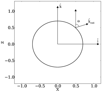
Figure 1.— Geometry of the gas distribution. The angular velocity vector is parallel to the unit vector $\hat{k}$. In order to describe the departures from spherical symmetry we use the polar angle $\theta$ formed by the direction of the outgoing photons with respect to the $z$-axis. We define define the variable $\mu\equiv\cos\theta$ to report to present our results. Computing the spectra for photons in a narrow range of $\mu$ is equivalent to having a line-of-sight oriented in that direction.

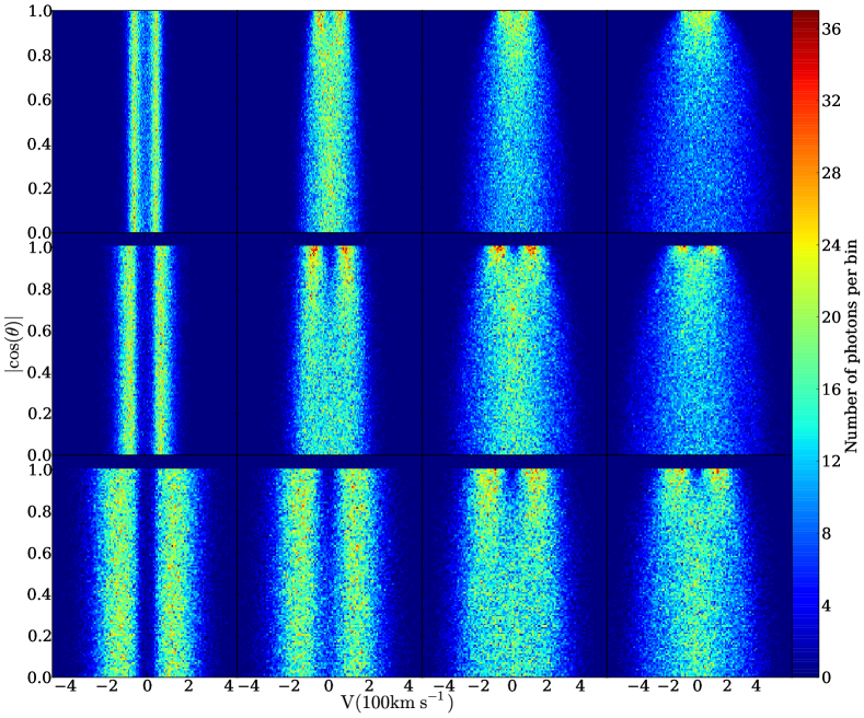
Figure 2.— 2D histogram showing the number of photons that escape with frequency $x$ forming an angle $\theta$ (parametrized as $|\cos\theta|$) with the rotation axis. The rotational velocity ($0,100,200,300$ km s^-1) increases from left to right and the optical depth ($10^{5}$, $10^{6}$, $10^{7}$) from top to bottom. The Ly$\alpha$ photons are initialized at the center of the sphere. Two main results can be read from this figure. First, the line morphology depends on the viewing angle. Second, the line can become single peaked for high rotational velocities.

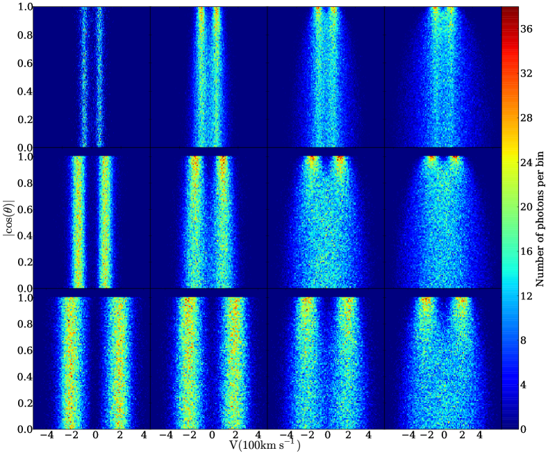
Figure 3.— Same as Fig. 2 for Ly$\alpha$ photons initialized homogeneously throughout the sphere.

Figure 4.— Shape of the Ly$\alpha$ line for different maximum rotational velocities for a LoS perpendicular to the rotation axis ($|\mu|\sim 0$). The continuous (dashed) line represents the central (homogeneous) source distributions. The continuous thin line represents the intrinsic homogeneous spectrum. The panels follow the same distribution as in Fig.s 2 and 3.

Figure 5.— Shape of the Ly$\alpha$ line for different maximum rotational velocities for a LoS perpendicular to the rotation axis ($|\mu|\sim 1$). The continuous (dashed) line represents the central (homogeneous) source distributions. The continuous thin line represent the intrinsic homogeneous spectrum. The panels follow the same distribution as in Fig.s 2 and 3.

2.2. Brief Description of the Radiative Transfer Codes

Here we briefly describe the relevant characteristics of the two radiative transfer codes we have used. For a detailed description we refer the reader to the original papers Forero-Romero et al. (2011) and Dijkstra & Kramer (2012).

The codes follow the individual scatterings of Ly$\alpha$ photons as they travel through a 3D distribution of neutral Hydrogen. The frequency of the photon (in the laboratory frame) and its direction of propagation change at every scattering. This change in frequency is due to the peculiar velocities of the Hydrogen absorbing and re-emitting the photon. Once the photons escape the gas distribution we store their direction of propagation and frequency at their last scattering.

The initialization process for the Ly$\alpha$ photons specifies its position, frequency and direction of propagation. We select the initial frequency to be exactly the Ly$\alpha$ rest-frame frequency in the gas reference frame and the direction of propagation to be random following an flat probability distribution over the sphere. It means that for photons emitted from the center of the sphere $x_{\rm in}=0$, while photons emitted at some radii with a peculiar velocity $\vec{v}$ have initial values $x_{\rm in}$ depending on its direction of propagation: $x_{\rm in}=\vec{v}\cdot\hat{k}_{\rm in}/v_{\rm th}$. We do not include the effect of turbulent velocities in the initialization. We neglect this given that the induced perturbation should be on the close to the thermal velocity, $12.8$ km s^-1, which is one order of magnitude smaller than the velocity widths ($100$-$500$ km s^-1) in the static case.

If dust is present, the photon can interact either with a Hydrogen atom or dust grain. In the case of a dust interaction the photon can be either absorbed or scattered. This probability is encoded in the dust albedo, $A$, which we chose to be $1/2$. In order to obtain accurate values for the escape fraction of photons in the presence of dust, we do not use any accelerating mechanism in the radiative transfer.

The codes treat the gas as homogeneous in density and temperature. This implies that the gas is completely defined by its geometry (i.e. sphere or slab), temperature $T$, Hydrogen optical depth $\tau_{\rm H}$, dust optical depth $\tau_{\rm a}$ and the bulk velocity field $\vec{v}$.

2.3. Grid of Simulated Galaxies

In the Monte Carlo calculations we follow the propagation of $N_{\gamma}=10^{5}$ numerical photons through different spherical galaxies. For each galaxy we vary at least one of the following parameters: the maximum rotational velocity $V_{\rm max}$, the hydrogen optical depth $\tau_{H}$, the dust optical depth $\tau_{a}$ and the initial distribution of photons with respect to the gas. In total there are $48$ different models combining all the possible different variations in the input parameters. Table 1 lists the different parameters we used to generate the models. The results and trends we report are observed in both Monte Carlo codes.

Physical Parameter (units)	Symbol	Values
Velocity ( km s-1)	$V_{\rm max}$	$0,\ \ 100,\ 200,\ 300$
Hydrogen Optical Depth	$\tau_{H}$	$10^{5},\ 10^{6},\ 10^{7}$
Dust Optical Depth	$\tau_{a}$	$0$,$1$
Photons Distributions		Central, Homogeneous

Table 1 Summary of Physical Parameters of our Monte Carlo Simulations.

3. Results

The main results of this paper are summarized in Fig. 2 and 3. They show 2D histograms of the escape frequency $x$ and outgoing angle $\theta$ parametrized by $|\mu|$. Taking into account only photons photons around a value of $|\mu|$ gives us the emission detected by an observer located at an angle $\theta$ with respect to the rotation axis. We have verified that the solutions are indeed symmetric with respect to $\mu=0$. We have also verified that the total flux is the same for all $\mu$.

From these figures we can see that the line properties change with rotational velocity and depend on the viewing angle $\theta$. In the next subsections we quantify the morphology changes with with velocity, optical depth and viewing angle. We characterize the line morphology by its total intensity, the full width at half maximum, (FWHM) and the location of the peak maxima. In order to interpret the morphological changes in the line we also report the median number of scatter for each Ly$\alpha$ photon in the simulation. For the models where dust is included we measure the escape fraction as a function of rotational velocity and viewing angle.

3.1. Line Morphology

The first column in both Fig. 2 and 3 shows that for the static sphere the line properties are independent of $|\mu|$, as it is expected due to the spherical symmetry. However, for increasing rotational velocities, at a fixed optical depth, there are clear signs that this symmetry is broken.

If the viewing angle is aligned with the rotation axis, $|\mu|\sim 1$, the Ly$\alpha$ line keeps a double peak with minor changes in the morphology as the rotational velocity increases. However, for a line of sight perpendicular to the rotation axis, $|\mu|\sim 0$, the impact of rotation is larger. The double peak readily transforms into a single peak.

This is clear in Fig. 4 where we present the different line morphologies for $|\mu|\sim 0$ in the homogeneous and central configurations. The panels have the same distribution as Fig. 2 and 3. There are three clear effects on the line morphology as the rotational velocity increases. First, the line broadens; second, the double peaks reduce their intensity; and third, the intensity at the line centre rises. The last two effects are combined to give the impression that the double peaks are merged into a single one at high rotational velocities.

3.2. Integrated Line Intensity

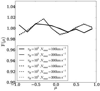
Figure 6.— Integrated flux distribution as a function of the viewing angle as parametrized by $\mu$. Continuous (dashed) correspond to central (homogeneous) source distribution. The models correspond to an optical depth of $\tau_{\rm H}=10^{5}$ and rotational velocities of $100$ km s^-1, $200$ km s^-1and $300$ km s^-1. The distributions are flat in the range of models probed in this paper, meaning that the integrated flux for all viewing angles is the same.

We now consider possible variations in the integrated flux with respect to the viewing angle $\theta$. To this end we define the normalized flux seen by an observer at an angle $\mu$ by:

$$F(\mu)=\frac{2\Delta N}{N\Delta\mu},$$ (4)

where $\mu=\cos\theta$, $N$ is the total number of outgoing photons, $\Delta N$ is the number of photons in an angular bin $\Delta\theta$. This definition satisfies the condition $\int_{-1}^{1}F(\mu)d\mu/2=1$. In the case of perfect spherical symmetry one expects a flat distribution with $F(\mu)=1$.

Fig. 6 shows the results for a selection of models with $\tau_{\rm H}=10^{5}$, different rotational velocities and the two types of source distributions. This shows that $F(\mu)$ is consistent with being flat, apart from some statistical fluctuations on the order of 2%.

This is a remarkable result: while the rotation axis defines preferential direction, the integrated flux is the same for all viewing angles in the range of parameters explored in this paper. This can be understood from the fact that radiative transfer inside a sphere that undergoes solid-body rotation proceeds identical as inside a static sphere: we can draw a line between any two atoms within the rotating cloud, and their relative velocity along this line is zero (apart from the relative velocity as a result of random thermal motion), irrespective of the rotation velocity of the cloud. This relative velocity is what is relevant for the radiative transfer

3.3. Full Width at Half Maximum

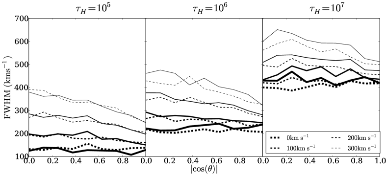
Figure 7.— FWHM for the non-dusty models as a function of the viewing angle parametrized by $|\cos\theta|$. Continuous (dashed) lines correspond to central (homogeneous) source distributions. The general trend is of an decreasing line width as the line of sight becomes parallel to the rotation axis.

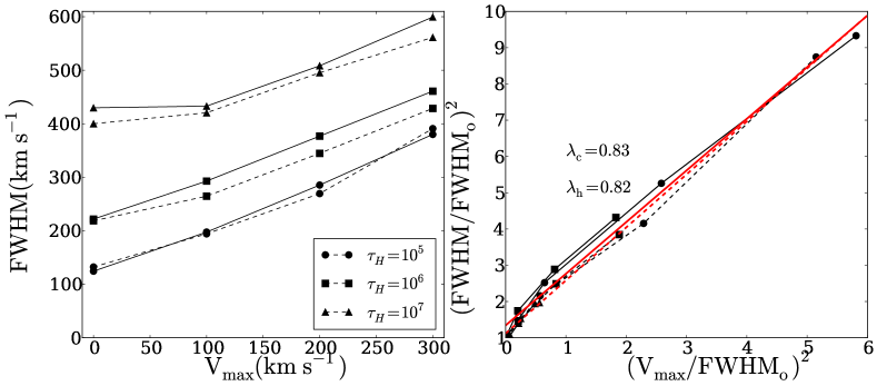
Figure 8.— FWHM for the non-dusty models as a function of rotational velocity $V_{\rm max}$ for observers located perpendicular to the rotation axis. The left panel shows the results in velocity units while the right panel normalizes the data by the FWHM in the static case. Continuous (dashed) lines correspond to central (homogeneous) source distributions. The straight lines represent the fit to the data using the expression in Eq. (5).

We use the full width at half maximum (FWHM) to quantify the line broadening. We measure this width from the line intensity histogram by finding the values of the velocities at half maximum intensity. We use lineal interpolation between histogram points to get a value more precise than the bin size used to construct the histogram.

Fig. 7 shows the FWHM for all models as a function of the viewing angle. The FWHM increases for decreasing values of $\mu$ (movement from the poles to the equator) and increasing values of $V_{\rm max}$. In Fig. 8 we fix $|\mu|<0.1$, i.e. viewing angle perpendicular to the rotation axis, to plot the FWHM as a function of rotational velocity.

We parametrize the dependency of the line width with $V_{\rm max}$ as

$${\rm FWHM}^{2}={\rm FWHM}_{0}^{2}+V_{\rm max}^{2}/\lambda^{2},$$ (5)

where FWHM₀ is the velocity width in the static case and $\lambda$ is a positive scalar to be determined as a fit to the data. With this test we want to know to what extent the new velocity width can be expressed as a quadratic sum of the two relevant velocities in the problem.

All the models fall into a single family of lines in the plane shown in the right panel of Fig. 8, justifying the choice of our parametrization. We fit simultaneously all the points in two separate groups, central and homogeneous sources. We find that these values are $\lambda_{\rm c}=0.83\pm 0.06$ and $\lambda_{\rm h}=0.82\pm 0.05$ respectively.

3.4. Line Maxima

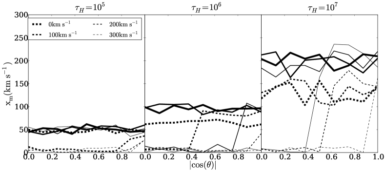
Figure 9.— Position of the line maxima as a function of maximum rotational velocity $V_{\rm max}$. Continuous (dashed) lines correspond to central (homogeneous) source distributions. A value of $x_{\rm max}=0$ indicates that line becomes single peaked.

We measure the peak maxima position, $x_{m}$, to quantify the transition from double into single peak profiles. In Fig. 9 we show the dependence of $x_{m}$ with the viewing angle parametrized by $|\cos\theta|$ for different rotational velocities. There are two interesting features that deserve attention. First, for a viewing angle parallel to the rotational axis ($\mu\sim 1.0$) the maxima of all models with the same kind of source initialization are similar regardless of the rotational velocity. Second, at a viewing angle perpendicular to the rotation axis ($\mu\sim 0.0$) a large fraction of models become single peaked. This feature appears more frequently for homogeneously distributed sources if all the other parameters are equal.

3.5. Dusty Clouds: Escape Fraction

Source	$\tau_{H}$		$\ V_{\rm max}$
Distribution			( km s-1)
		0	100	200	300
Homogeneous	$10^{5}$	0.263	0.263	0.263	0.263
	$10^{6}$	0.291	0.292	0.293	0.293
	$10^{7}$	0.228	0.228	0.228	0.228
Central	$10^{5}$	0.096	0.096	0.096	0.096
	$10^{6}$	0.066	0.066	0.066	0.066
	$10^{7}$	0.015	0.016	0.016	0.015

Table 2 Escape fraction values for all dusty models.

We now estimate the escape fraction $f_{\rm esc}$ for the dusty models. The main result is that we do not find any significant dependence with either the viewing angle nor the rotational velocity. This is consistent with our finding in § 3.2, that radiative transfer inside the cloud does not depend on its rotational velocity. For completeness we list in Table 2 the escape fraction for all models.

We now put these results in the context of the analytic solution for the infinite slab(Neufeld, 1990). In Neufeld’s set-up the analytic solution depends uniquely on the product $(a\tau_{\rm H})^{1/3}\tau_{A}$ where $\tau_{A}=(1-A)\tau_{a}$, valid only in the limit $a\tau_{\rm H}\gg 1$. At fixed values of $\tau_{a}$ the escape fraction monotonically decreases with increasing values of $\tau_{\rm H}$. This expectation holds for the central sources. But in the case of homogeneous sources the escape fraction increases slightly from $\tau_{\rm H}=10^{5}$ to $\tau_{\rm H}=10^{6}$

The naive interpretation of the analytic solution does not seem to hold for photons emitted far from the sphere’s center. We suggest that increasing $\tau_{\rm H}$ from $10^{5}$ to $10^{6}$ causes a transition from the ’optically thick’ to the ’extremely optically thick’ regime for a noticeable fraction of the photons in the homogeneous source distribution.

In the optically thick regime, Ly$\alpha$ photons can escape in ’single flight’ which corresponds to a scenario in which the photon resonantly scatters $10^{4}-10^{5}$ times until it is scattered into the wing of the line ($x\sim 3-4$). At these frequencies the medium is optically thin, and the photons can escape efficiently in a single flight. In contrast, in an extremely optically thick medium Ly$\alpha$ photons escape in a ‘single excursion’ (Adams, 1972). Here, photons that are scattered into the wing of the line escape from the medium in a sequence of wing scattering events. In both cases, Ly$\alpha$ photons resonantly scatter $10^{4}$-$10^{5}$ times. Because we keep our clouds the same size, the mean free path of Lya photons that scatter resonantly is 10 times larger for the case $\tau_{\rm H}=10^{5}$ than for $\tau_{\rm H}=10^{6}$. If we compute the average distance $D$ travelled by Ly$\alpha$ photons through a medium of size $R$ as a function of line center optical depth $\tau_{\rm H}$, then we find that during the transition from optically thick to extremely optically thick the mean traversed distance $D$ actually decreases slightly. This decrease is unique to this transition region, and $D$ generally increases with $\tau_{\rm H}$ at other values of $\tau_{\rm H}$.

3.6. Average Number of Scatterings

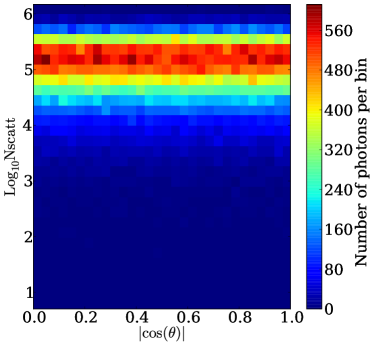
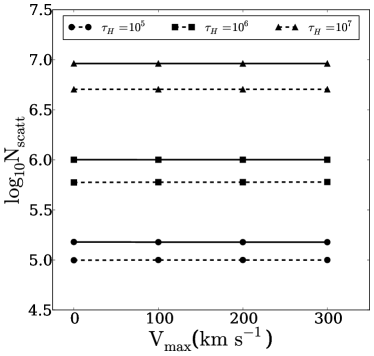
Figure 10.— 2D histogram of the logarithm of the average number of scatterings as function of $\mu$ (left) and the maximum rotational velocity $V_{\rm max}$ (right). The left panel shows the behaviour for $\tau=10^{5}$ and $V_{max}=300$ km s^-1as a function of $\left|\cos\theta\right|$, the color indicates the number of photons per bin. In the right panel the continous (dashed) lines represent the results for the central (homogeneous) model. The independence of $N_{\rm scatt}$ with $\mu$ and $V_{\rm max}$ is present in all models.

The number of scatterings affects the escape frequency of a Ly$\alpha$ photon. Studying this quantity further illustrates the independence of the integrated flux and the escape fraction on rotational velocity.

In Fig. 10 we show the average number of scatterings $\langle N_{\rm scatt}\rangle$ as a function of the cosinus of the outgoing angle $|\cos\theta|$ and the rotational velocity $V_{\rm max}$. From the right panel observe that the number of scatterings and the outgoing angle are independent. This plot corresponds to the specific case of the central model with $\tau=10^{5}$ and $V_{\rm max}=300$ km s^-1, but we have verified that this holds for all models.

The right panel of Fig. 10 shows how the average number of scatterings is also independent from the rotational velocity. The lower number of average scatterings in the homogeneous source distribution is due to a purely geometrical effect. Photons emitted close to the surface go through less scatterings before escaping.

In static configurations it is expected that the optical depth correlates number of scatterings. This has been precisely quantified in the case of static infinite slab. In that model for centrally emitted sources the average number of scatterings depends only on the optical depth $\langle N_{\rm scatt}\rangle=1.612\tau_{\rm H}$ (Adams, 1972; Harrington, 1973), for homogeneously distributed sources $\langle N_{\rm scatt}\rangle=1.16\tau_{\rm H}$ (Harrington, 1973).

In our case we find that for the central model the number of scatterings is proportional to the optical depth, with $\langle N_{\rm scatt}\rangle=(1.50,1.00,0.92)\tau_{\rm H}$ for optical depth values of $\tau_{\rm H}=(10^{5},10^{6},10^{7})$ respectively. For the homogeneous sources we find that $\langle N_{\rm scatt}\rangle=(0.99,0.59,0.51)\tau_{\rm H}$.

4. Discussion

4.1. Towards an analytical description

There is a key result of our simulations that allows us to build an analytical description for the outgoing spectra. It is the independence of the following three quantities with the rotational velocity and the viewing angle: integrated flux, average number of scatterings and escape fraction.

As we explained in § 3.2, the best way to understand this is that radiative transfer inside a sphere that undergoes solid-body rotation proceeds identical to that inside a non-rotating sphere. While scattering events off atoms within the rotating cloud impart Doppler boosts on the Ly$\alpha$ photon, these Doppler boost are only there in the lab-frame. Therefore, in the frame of the rotating gas cloud all atoms are stationary with respect to each other and the scattering process proceeds identical as in the static case (also see § 3.2 for an additional more quantitative explanation).

This result allows us to analytically estimate the spectrum emerging from a rotating cloud: The spectrum of Lyman $\alpha$ photons emerging from a rotating gas cloud is identical as for the static case in a frame that is co-rotating with the cloud. However, the surface of cloud now moves in the lab-frame. Each surface-element on the rotating cloud now has a bulk velocity with respect to a distant observer. In order to compute the spectrum one can integrate over all the surface elements in the sphere with their corresponding shift in velocity and an additional weight by the surface intensity.

Fig 11 shows some examples of analytic versus full MC spectra using this approach (the implementation details are in the Appendix). The left panel shows the results for different rotational velocities in the case of $\tau_{H}=10^{7}$ and an observer located perpendicular to the axis of rotation ($i=0$ in the scheme of Fig 12 in the Appendix). The right panel shows the results for different viewing angles in the case of $\tau_{H}=10^{7}$ and a rotational velocity of $V_{\rm max}=300$ km s^-1.

The two methods clearly give good agreement, though not perfect. In particular, the left panel shows that the MC gives rise to a spectrum that is slightly more concentrated towards the line centre. As we explain in Appendix A, we do not expect perfect agreement, because this requires an analytic solution for the spectrum of Ly$\alpha$ photons emerging from a static, optically extremely thick cloud as a function of the angle at which they escape from the sphere. This solution does not exist in the literature. It is possible to get better agreement my modifying the surface brightness profile. In any case, the analytic calculation closely captures the results obtained from the full calculations from the MC simulations. As such, they are extremely useful and provide us with a quick tool to verify our calculations at the first order level.

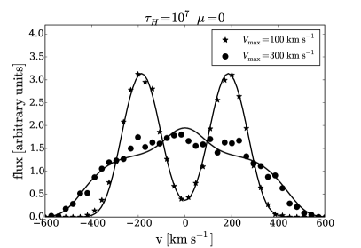
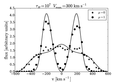
Figure 11.— Comparison of the Monte Carlo results against the analytic solution. The left panel explores the results of different velocities. The right panel presents the results for two different observers: paralel and perpendicular to the rotational axis, $\mu=1$ and $\mu=0$ respectively.

4.2. Impact on the interpretation of simulated and observational data

We now compare our findings to other computational results and discuss its possible implications for the interpretation of observational data.

Escape at Line Center. Our models have shown that rotation enhances the flux density at line center (see Fig. 4). It has recently been proposed that galaxies with Lya spectral lines that contain flux at line center may be ‘leaking’ ionizing (LyC) photons (Behrens et al., 2014; Verhamme et al., 2014). The main reason for this possible connection is that the escape of ionizing (LyC) photons requires $N_{\rm HI}<10^{17}$cm^-2. The same low column densities facilitate the escape of Ly$\alpha$ photons at (or close to) line center. Our work suggests that rotation may provide an alternative explanation.

Single peaked lines. The presence of single peaked profiles has been associated to inflow/outflow dynamics (Verhamme et al., 2006; Dijkstra & Kramer, 2012). Gas bulk rotation can also be considered as a probable origin for that behaviour, provided that the observed single peak is highly symmetric. Similarly, in the case of double peaked lines with a high level of flux at the line center, rotation also deserves to be considered in the pool of possible bulk flows responsible for that feature, specially if the two peaks have similar intensities.

Systemic velocities. There are observational measurements for the velocity shift between the Ly$\alpha$ and other emission lines. In our study we find that the position of the peak maxima can suddenly change with rotation and viewing angle. Namely the line can become single peaked for high rotational velocities and viewing angles perpendicular to the rotation axis.

Galaxy simulations with gas rotation. Verhamme et al. (2012) studied Ly$\alpha$ line emission in two high resolution simulations of individual galaxies. The main purpose of their study was to assess the impact of two different ISM prescriptions. However, each simulated galaxy had a disc structure with a clear rotation pattern in the ISM and inflowing gas from the circum-galactic region. The configuration had an axial symmetry and they reported a strong dependence of both the escape fraction and the total line intensity as a function of the $\theta$ angle. From our study, none of these two quantities has a dependence either on the inclination angle or the rotational velocity. We suggest that he effect reported by Verhamme et al. (2012) is consistent with being a consequence of the different hydrogen optical depth for different viewing angles and not as an effect of the bulk rotation.

Zero impact on the Ly$\alpha$ escape fraction. Study of high redshift LAEs in numerical simulation often requires the estimation of the Ly$\alpha$ escape fraction in order to compare their results against observations (Forero-Romero et al., 2011; Dayal & Ferrara, 2012; Forero-Romero et al., 2012; Orsi et al., 2012; Garel et al., 2012). Most of these models estimate the escape fraction from the column density of dust and neutral Hydrogen. The results of our simulation indicate that the rotational velocity does not induce additional uncertainties in those estimates.

5. Conclusions

In this paper we quantified for the first time in the literature the effects of gas bulk rotation in the morphology of the Ly$\alpha$ emission line in star forming galaxies. Our results are based on the study of an homogeneous sphere of gas with solid body rotation. We explore a range of models by varying the rotational speed, hydrogen optical depth, dust optical depth and initial distribution of Ly$\alpha$ photons with respect to the gas density. As a cross-validation, we obtained our results from two independently developed Monte-Carlo radiative transfer codes.

Two conclusions stand out from our study. First, rotation clearly impacts the Ly$\alpha$ line morphology; the width and the relative intensity of the center of the line and its peaks are affected. Second, rotation introduces an anisotropy for different viewing angles. For viewing angles close to the poles the line is double peaked and it makes a transition to a single peaked line for high rotational velocities and viewing angles along the equator. This trend is clearer for spheres with homogeneously distributed radiation sources than it is for central sources.

Remarkably, we find three quantities that are invariant with respect to the viewing angle and the rotational velocity: the integrated flux, the escape fraction and the average number of scatterings. These results helped us to construct the outgoing spectra of a rotating sphere as a superposition of spectra coming from a static configuration. This description is useful to describe the main quantitative features of the Monte Carlo simulations.

Quantitatively, the main results of our study are summarized as follows.

• In all of our models, rotation induces changes in the line morphology for different values of the angle between the rotation axis and the LoS, $\theta$. The changes are such that for a viewing angle perpendicular to the rotation axis, and high rotational velocities the line becomes single peaked.

• The line width increases with rotational velocity. For a viewing angle perpendicular to the rotation axis This change approximately follows the functional form ${\rm FWHM}^{2}={\rm FWHM}_{0}^{2}+(V_{\rm max}/\lambda)^{2}$, where FWHM₀ indicates the line width for the static case and $\lambda$ is a constant. We have determined this constant to be $\lambda_{\rm c}=0.83\pm 0.06$ and $\lambda_{\rm h}=0.82\pm 0.05$ for the central and homogeneous source distributions, respectively.

• At fixed rotational velocity the line width decreases as $|\mu|$ increases, i.e. the smallest value of the line width is observed for a line of sight parallel to the ration axis.

• The single peaked line emerges at viewing angles $\mu\sim 1$ for when the rotational velocity is close to than half the FWHM₀.

Comparing our results with recent observed LAEs we find that morphological features such as high central line flux, single peak profiles could be explained by gas bulk rotation present in these LAEs.

The definitive and clear impact of rotation on the Ly$\alpha$ morphology suggests that this is an effect that should be taken into account at the moment of interpreting high resolution spectroscopic data. In particular it is relevant to consider the joint effect of rotation the and ubiquitous outflows (Remolina-Gutierrez et al., in prep.) because rotation can lead to enhanced escape of Ly$\alpha$ at line center, which has also been associated with escape of ionizing (LyC) photons (Behrens et al., 2014; Verhamme et al., 2014)

Appendix A Analytic Expression for the Ly$\alpha$ Spectrum emerging from Rotating Cloud

Ly$\alpha$ scattering through an optically thick gas cloud that is undergoing solid-body rotation (i.e. in which the angular speed around the rotation axis is identical for each hydrogen atom) proceeds identical as in a static cloud. In order to compute the spectrum emerging from a rotating cloud, we sum the spectra emerging from all surface elements of the cloud, weighted by their intensity.

We adopt the geometry shown in Fig 12 to derive an analytic expression of this emerging spectrum, Note that this geometry differs from the scheme shown in Fig 1 in the main body of the paper.

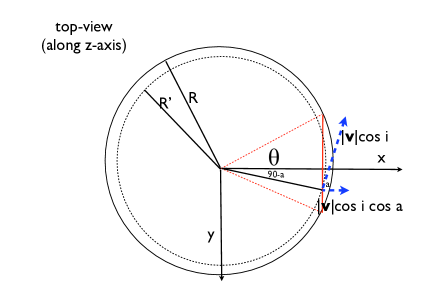
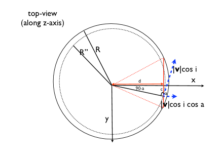
Figure 12.— Adopted geometry for evaluating the analytic spectrum.

The sightline to the observer & rotation axis define the $x-z$ plane. The left panel in Fig 12 shows the view from the $y$-axis. The observer sits along the $x$ axis. The rotation axis makes an angle $i$ with respect to the $z$-axis. We sum up spectra from individual patches by integrating over the impact parameter $b$, and angle $\phi$. Each $(b,\phi)$ corresponds to a point on the sphere. This point has a velocity vector ${\bf v}(b,\phi,i)$, which we denote with ${\bf v}$ for brevity. The magnitude of ${\bf v}$ is $|{\bf v}|=V_{\rm max}R^{\prime}/R$. Here $R^{\prime}=\sqrt{R^{2}-s^{2}}$, in which $s$ denotes the distance of the point $(b,\phi)$ to the plane perpendicular to the rotation axis and through the origin (see the left panel of Fig 12). This distance $s$ is given by $s=|-\sin i\sqrt{R^{2}-b^{2}}+b\cos\phi\cos i|$.

The spectrum of the flux emerging from the surface at point $(b,\phi)$ is

$$J(x,b,\phi,i)=\frac{\sqrt{\pi}}{\sqrt{24}a\tau_{0}}\Bigg{(}\frac{(x-x_{\rm b})^{2}}{1+{\rm cosh}\Big{[}\sqrt{\frac{2\pi^{3}}{27}}\frac{|(x-x_{\rm b})^{3}|}{a\tau_{0}}\Big{]}}\Bigg{)},$$

where $x_{b}\equiv v_{b}/v_{\rm th}$, and $v_{b}$ is the component of ${\bf v}$ projected onto the line-of-sight. This component is given by

$$v_{\rm b}(b,\phi,i)=V_{\rm max}\frac{\sqrt{R^{2}-s^{2}}}{R}\cos i{\hskip 2.84526pt}\cos a,$$ (A1)

where $\beta=90^{\circ}-a$. The factor $\cos i$ accounts for the projection onto the $x-y$ plane, and the factor $\cos a$ for the subsequent projection onto the line-of-sight. The right panel of Fig. 12 shows that this angle $a$ can be computed from

$$\tan\beta=\tan[90^{\circ}-a]=\frac{c}{d}=\frac{b\sin\phi}{\sqrt{R^{2}-b^{2}}},$$ (A2)

In order to compute to total intensity we integrate over $b$ and $\phi$ with a weight given by the surface brightness of the sphere at $(b,\phi)$, $S(b,\phi)$.

$$J(x,i)=2\pi\int_{0}^{R}db{\hskip 2.84526pt}b\int_{0}^{2\pi}d\phi{\hskip 2.84526pt}S(b,\phi)J(x,b,\phi,i)\approx 2\pi\int_{0}^{R}db{\hskip 2.84526pt}b\int_{0}^{2\pi}d\phi{\hskip 2.84526pt}J(x,b,\phi,i)\\ .$$

In the last expression we assume that $S(b,\phi)$ is constant. This corresponds to $I(\mu)\propto\mu$ at the surface, where $\mu$ denotes the cosine of the angle of the propagation direction of the outgoing photon and the normal to the spheres surface: a fixed $db$ corresponds to a physical length $ds=db/\mu$ on the sphere. If $I(\mu)$ were constant, this would imply that the sphere should appear brighter per unit $b$. A constant surface brightness profile requires the directional dependence for $I(\mu)\propto\mu$ to correct for this. Indeed, this is what is expected for the escape of Ly$\alpha$ photons from static, extremely opaque media (see Ahn et al. (2001); their Fig 4 and accompanying discussion).

It is worth stressing that this derivation should not be viewed as a complete analytic calculation, and we do not expect perfect agreement: we assumed a functional form for the surface brightness profile [or for $I(\mu)$]. Moreover, $I(\mu)$ itself may depend on frequency $x$. In other words, analytic solutions exist for $J(x)=\int_{0}^{1}I(x,\mu)d\mu$ at the boundary of the sphere, and approximate expressions for $I(\mu)=\int dxI(x,\mu)$, but not for $I(x,\mu)$ itself. The spectra we obtained from the Monte-Carlo calculations naturally include the proper $I(x,\mu)$, and are therefore expected to be more accurate.

To further test the assumption of scattering in a rotating medium proceeding as in a static medium we compute the distribution of the outgoing angles $\mu$. The results are shown in Figure 13; it shows that the distribution for $\mu$ is independent of the rotational velocity and the location over the sphere. The only dependence comes with $\tau_{H}$. For higher values of the optical depth the distribution gets closer to $I(\mu)\propto\mu$ as expected for a static medium (Ahn et al., 2001).

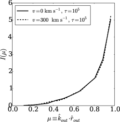
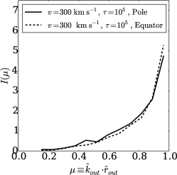
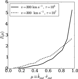
Figure 13.— Distribution of the cosine of the angle between the propagation direction and a vector normal to the sphere’s surface. The distributions have been normalized to unity. Left panel: different rotational velocities; middle panel: different viewing angles; right panel: different optical depths. Only the optical depth has an effect on the distribution of outogoing directions. This is consistent with the assumption that Lyman $\alpha$ scattering in a medium with solid body rotation proceeds as in a static medium.

References

- Adams (1972) Adams, T. F. 1972, ApJ, 174, 439
- Ahn et al. (2000) Ahn, S.-H., Lee, H.-W., & Lee, H. M. 2000, Journal of Korean Astronomical Society, 33, 29
- Ahn et al. (2001) —. 2001, ApJ, 554, 604
- Ahn et al. (2003) —. 2003, MNRAS, 340, 863
- Auer (1968) Auer, L. H. 1968, ApJ, 153, 783
- Avery & House (1968) Avery, L. W., & House, L. L. 1968, ApJ, 152, 493
- Barnes et al. (2011) Barnes, L. A., Haehnelt, M. G., Tescari, E., & Viel, M. 2011, MNRAS, 416, 1723
- Behrens et al. (2014) Behrens, C., Dijkstra, M., & Niemeyer, J. C. 2014, A&A, 563, A77
- Behrens & Niemeyer (2013) Behrens, C., & Niemeyer, J. 2013, A&A, 556, A5
- Dayal & Ferrara (2012) Dayal, P., & Ferrara, A. 2012, MNRAS, 421, 2568
- Dijkstra (2014) Dijkstra, M. 2014, ArXiv e-prints, arXiv:1406.7292
- Dijkstra et al. (2006) Dijkstra, M., Haiman, Z., & Spaans, M. 2006, ApJ, 649, 14
- Dijkstra & Kramer (2012) Dijkstra, M., & Kramer, R. 2012, MNRAS, 424, 1672
- Finkelstein et al. (2013) Finkelstein, S. L., Papovich, C., Dickinson, M., Song, M., Tilvi, V., Koekemoer, a. M., Finkelstein, K. D., Mobasher, B., Ferguson, H. C., Giavalisco, M., Reddy, N., Ashby, M. L. N., Dekel, a., Fazio, G. G., Fontana, a., Grogin, N. a., Huang, J.-S., Kocevski, D., Rafelski, M., Weiner, B. J., & Willner, S. P. 2013, Nature, 502, 524
- Forero-Romero et al. (2011) Forero-Romero, J. E., Yepes, G., Gottlöber, S., Knollmann, S. R., Cuesta, A. J., & Prada, F. 2011, MNRAS, 415, 3666
- Forero-Romero et al. (2012) Forero-Romero, J. E., Yepes, G., Gottlöber, S., & Prada, F. 2012, MNRAS, 419, 952
- Garel et al. (2012) Garel, T., Blaizot, J., Guiderdoni, B., Schaerer, D., Verhamme, A., & Hayes, M. 2012, MNRAS, 422, 310
- Gawiser et al. (2007) Gawiser, E., Francke, H., Lai, K., Schawinski, K., Gronwall, C., Ciardullo, R., Quadri, R., Orsi, A., Barrientos, L. F., Blanc, G. A., Fazio, G., & Feldmeier, J. J. 2007, ApJ, 671, 278
- Hansen & Oh (2006) Hansen, M., & Oh, S. P. 2006, MNRAS, 367, 979
- Harrington (1973) Harrington, J. P. 1973, MNRAS, 162, 43
- Hunter (2007) Hunter, J. D. 2007, Computing In Science & Engineering, 9, 90
- Koehler et al. (2007) Koehler, R. S., Schuecker, P., & Gebhardt, K. 2007, A&A, 462, 7
- Laursen et al. (2009) Laursen, P., Sommer-Larsen, J., & Andersen, A. C. 2009, ApJ, 704, 1640
- Loeb & Rybicki (1999) Loeb, A., & Rybicki, G. B. 1999, ApJ, 524, 527
- Neufeld (1990) Neufeld, D. A. 1990, ApJ, 350, 216
- Orsi et al. (2012) Orsi, A., Lacey, C. G., & Baugh, C. M. 2012, MNRAS, 425, 87
- Ouchi et al. (2008) Ouchi, M., Shimasaku, K., Akiyama, M., Simpson, C., Saito, T., Ueda, Y., Furusawa, H., Sekiguchi, K., Yamada, T., Kodama, T., Kashikawa, N., Okamura, S., Iye, M., Takata, T., Yoshida, M., & Yoshida, M. 2008, ApJS, 176, 301
- Partridge & Peebles (1967) Partridge, R. B., & Peebles, P. J. E. 1967, ApJ, 147, 868
- Pérez & Granger (2007) Pérez, F., & Granger, B. E. 2007, Computing in Science and Engineering, 9, 21
- Rhoads et al. (2000) Rhoads, J. E., Malhotra, S., Dey, A., Stern, D., Spinrad, H., & Jannuzi, B. T. 2000, ApJ, 545, L85
- Schenker et al. (2012) Schenker, M. A., Stark, D. P., Ellis, R. S., Robertson, B. E., Dunlop, J. S., McLure, R. J., Kneib, J.-P., & Richard, J. 2012, ApJ, 744, 179
- Verhamme et al. (2012) Verhamme, A., Dubois, Y., Blaizot, J., Garel, T., Bacon, R., Devriendt, J., Guiderdoni, B., & Slyz, A. 2012, A&A, 546, A111
- Verhamme et al. (2014) Verhamme, A., Orlitova, I., Schaerer, D., & Hayes, M. 2014, ArXiv e-prints
- Verhamme et al. (2006) Verhamme, A., Schaerer, D., & Maselli, A. 2006, A&A, 460, 397
- Yajima et al. (2012) Yajima, H., Li, Y., Zhu, Q., Abel, T., Gronwall, C., & Ciardullo, R. 2012, ApJ, 754, 118
- Yamada et al. (2012) Yamada, T., Nakamura, Y., Matsuda, Y., Hayashino, T., Yamauchi, R., Morimoto, N., Kousai, K., & Umemura, M. 2012, AJ, 143, 79
- Zheng & Miralda-Escudé (2002) Zheng, Z., & Miralda-Escudé, J. 2002, ApJ, 578, 33
- Zheng & Wallace (2013) Zheng, Z., & Wallace, J. 2013, ArXiv e-prints