Formation of Large-Amplitude Low-Frequency Waves in
Capillary Turbulence on Superfluid He-II

Abstract

The results of experimental and theoretical studies of the parametric decay instability of capillary waves on the surface of superfluid helium He-II are reported. It is demonstrated that in a system of turbulent capillary waves low-frequency waves are generated along with the direct Kolmogorov-Zakharov cascade of capillary turbulence. The effects of low-frequency damping and the discreteness of the wave spectrum are discussed.

I Introduction

Highly developed hydrodynamic turbulence has provided a fascinating challenge for engineers, physicists and mathematicians for over two hundred years. Turbulence appears in numerous systems ranging from planetary waves in the earth’s atmosphere to jet streams Smith and Lee (2005); Landa and McClintock (2004). Fully developed hydrodynamic turbulence can be formed by interacting vortices Frisch (1995). Turbulence may also appear in a system of nonlinearly interacting waves Zakharov et al. (1992); Nazarenko (2011), which is referred to as wave turbulence. The concept of wave turbulence originated from Peierls’ work Peierls (1929) on anharmonic crystals. Wave turbulence is manifested on planetary and interstellar scales, in the earth’s magnetosphere and its coupling with the solar wind Southwood (1978), in shock propagation in Saturn’s bow Scarf et al. (1981), and in interstellar plasmas Bisnovatyi-Kogan and Silich (1995). Fascinating atmospheric phenomena, such as auroras in the high-latitude regions of the earth, are caused by ion wave turbulence in magnetic flux tubes Southwood (1978). Wave turbulence also provides deep connections between the classical and quantum worlds; wave turbulence can result in kinetic condensation of classical waves Sun et al. (2012), which is similar in many ways to Bose-Einstein condensation in quantum systems such as ultra-cold atoms Seman et al. (2011).

Wave turbulence is much easier to understand than hydrodynamic turbulence, because it is appropriate when the building blocks of a system are linear waves that admit analytical descriptions. When the nonlinear interactions between waves may be treated as weak perturbations, the statistics of the system become tractable analytically. This allows one to derive the closed equation for the spectral energy density of the waves, called the kinetic equation. The kinetic equation for interacting waves has a steady-state scale invariant (power-law) solution that describes a constant flux of energy towards smaller scales. Such a power law spectrum can be viewed as the wave analog of the Kolmogorov spectrum of hydrodynamic turbulence Frisch (1995) and is referred to as the Kolmogorov-Zakharov (KZ) spectrum of wave turbulence Zakharov et al. (1992); Nazarenko (2011).

Surface capillary waves are the ripples that are created by a light breeze on the surface of a pond. They are short waves for which surface tension is the primary restoring force. The dispersion relation between the wave frequency $\omega$ and the wave number $k$ for capillary waves is

$$\omega(k)=\sqrt{\alpha k^{3}\over\rho},$$ (1)

where $\alpha$ is the surface tension and $\rho$ is the fluid density. For water, the characteristic wave length of capillary waves is less than $\lambda=2\pi\sqrt{\alpha/\rho g}\approx 1.7$ cm (where $g$ is the acceleration due to gravity). Capillary waves are a beautiful canonical example of a wave-turbulent system with weak nonlinear wave interactions. The Kolmogorov-Zakharov spectrum of capillary waves corresponds to the direct cascade, or flux of wave energy, from low to high wave frequencies. The existence and features of the KZ spectrum for capillary waves is well established through both experiments and theory Zakharov and Filonenko (1967); Pushkarev and Zakharov (1996); Henry et al. (2000); Brazhnikov et al. (2002); Kolmakov et al. (2004); Abdurakhimov et al. (2009).

We study capillary waves on the surface of superfluid helium. This system provides an ideal testbed for studying nonlinear wave dynamics due to its extremely low viscosity and the possibility of driving the fluid surface directly by an oscillating electric field, virtually excluding the excitation of bulk modes Brazhnikov et al. (2002). Previous experiments with waves on quantum fluids (liquid helium and hydrogen) allowed detailed study of the steady-state and decaying direct cascade of capillary turbulence Kolmakov et al. (2004); Abdurakhimov et al. (2009), modification of the turbulent spectrum by applied low-frequency driving Brazhnikov et al. (2005) and the turbulent bottleneck phenomena in the high-frequency spectral domain Abdurakhimov et al. (2010).

In this paper, we show that under certain conditions low-frequency waves on the fluid surface with frequencies lower than the driving frequency can be created in addition to the direct Kolmogorov-Zakharov cascade. In what follows we present our findings and discuss the mechanisms responsible for the low-frequency wave generation.

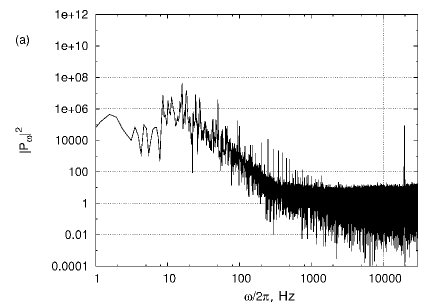
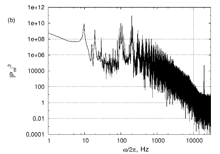
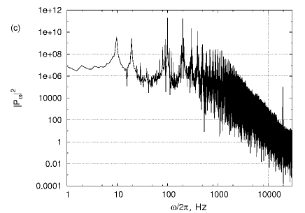
Figure 1: Long-time evolution of the spectrum of capillary turbulence. The spectra are shown for the moments (a) $t=1.31$ s, (b) 53.74 s and (c) 163.84 s after the driving force is turned on. Driving is applied at a frequency $\omega_{d}/2\pi=199$ Hz, the driving amplitude is $U_{d}=97$ V. Formation of low-frequency harmonics with $\omega<\omega_{d}$ are clearly seen in figures (b) and (c). The squared amplitudes of the harmonics $|P_{\omega}|^{2}$ are shown in arbitrary units.

II Experimental observations

The experimental arrangements were similar to those in our previous experiments with superfluid helium and liquid hydrogen Kolmakov et al. (2004); Abdurakhimov et al. (2009). In our experiments, helium ⁴He was condensed into a cylindrical cup formed by the bottom capacitor plate and a guard ring and was positioned in a helium cryostat. The cup has inner radius $R=30$ mm and depth $4$ mm. The experiments were conducted at temperature $T=1.7$ K of the superfluid liquid. The free surface of the liquid was positively charged as the result of $\beta$–particle emission from the radioactive plate located in the bulk liquid. Oscillations of the liquid surface were excited by application of an AC voltage $U(t)=U_{d}\sin(\omega_{d}t)$ to the lower capacitor’s plate in addition to the constant voltage. Oscillations of the fluid surface elevation $\zeta(\bm{r},t)$ were detected through variations of the power $P(t)$ of a laser beam reflected from the surface. (Here, $t$ is time and $\bm{r}$ is two-dimensional coordinates in the surface plane). The power $P(t)$ was measured with a photodetector and sampled with an analogue-to-digital converter. The capillary wave power spectrum $\zeta_{\omega}\propto P_{\omega}$ was calculated via the time Fourier transform of the signal $P(t)$ Brazhnikov et al. (2002). The measurements of wave damping in the cell showed that the quality factor at low frequencies $\omega<\omega_{d}$ is $Q\sim 10^{3}$. The finite size of the cell results in the discrete wave number spectrum. The capillary-to-gravity wave transition on the surface of superfluid helium is at frequency $\sim 30$ Hz. The surface oscillations with frequencies $\sim 30$ Hz are gravity-capillary waves, for which the restoring force is caused by both the capillary force and gravity. However, this frequency decreases at high pulling external electric fields normal to the surface Brazhnikov et al. (2002). The finite depth of the waves only influences the wave dispersion $\omega=\omega({k})$ at low frequencies $\omega<10$ Hz. The capillary wave length for liquid helium is $\lambda=0.17$ cm at $T=4.2$ K and increases to 0.3 cm for $T=1.7$ K.

Figure 1 shows formation of a wave-turbulent spectrum after switching on the driving force at the moment of time $t=0$. The driving frequency is $\omega_{d}/2\pi=199$ Hz. In Fig. 1a, waves with the frequency $\omega_{d}$ and its high-frequency harmonics begin to form on the noisy background. The latter is caused by mechanical vibrations of the installation. In Fig. 1b,c the Kolmogorov-Zakharov direct cascade of capillary turbulence is formed at $\omega>\omega_{d}$. It corresponds to transfer of the wave energy in a cascade-like manner towards higher frequency, in full agreement with our previous observations Brazhnikov et al. (2002); Kolmakov et al. (2004); Brazhnikov et al. (2005); Abdurakhimov et al. (2009, 2010). At frequencies $\omega/2\pi\sim 20$ kHz, the cascade is cut due to viscous damping in the fluid. The peak at $20.5$ kHz is caused by the noise of the He-Ne laser output power.

It is seen in Fig. 1b,c that low-frequency waves with $\omega<\omega_{d}$ are formed at large time $t\geq 50$ s after the drive is turned on. Specifically, the squared amplitude of the harmonics at $\omega_{d}/2\pi=99$ Hz is $|P_{\omega}|^{2}\approx 8.3\times 10^{9}$ a.u at $t=53.74$ s (Fig. 1b), and it reaches $|P_{\omega}|^{2}\approx 2.2\times 10^{11}$ a.u. at $t=163.84$ s (Fig. 1c). It is remarkable that in Fig. 1c, the amplitude of the subharmonics is larger than that for the wave at the drive frequency, which is $|P_{\omega}|^{2}\approx 1.5\times 10^{11}$ a.u. The amplitudes of the low-frequency harmonics at $\omega/2\pi\approx 10$ Hz shown in Fig. 1c are larger than the amplitudes of the high-frequency waves in the direct cascade with $\omega/2\pi\geq 500$ Hz. It is worth noting that formation of the low-frequency harmonics on a turbulent capillary-wave background has not yet been reported in the literature.

Generation of low-frequency waves shown in Fig. 1 can be attributed to the development of the decay instability of capillary waves at enough large wave amplitudes. The origin of this instability is in the modulation of a nearly periodic wave due to nonlinearity. This specific mechanism was earlier proposed to account for the creation of giant low-frequency waves on the water surface Dyachenko and Zakharov (2005); Onorato et al. (2001). It was also demonstrated that for waves on an ideal fluid with no damping, development of the decay instability should result in formation of a thermodynamic-equilibrium wave distribution $|P_{\omega}|^{2}\propto\Theta/\omega(k)$ where $\Theta$ is the effective temperature Balkovsky et al. (1995). However, it is seen in Fig. 1 that the observed spectrum at $\omega<\omega_{d}$ significantly differs from the proposed theoretical equilibrium spectrum.

III Numerical simulations

To understand the formation of large-amplitude low-frequency waves, we performed numerical modeling of the wave dynamics in the cylindrical cell with external driving and viscous damping. In the simulations, the deviation of the surface from the equilibrium flat state is expressed by time-dependent amplitudes $a_{k}(t)$ of the normal modes Zakharov and Filonenko (1967). We assume angular symmetry of the surface, so its deviation for capillary waves is $\zeta(r,t)=\sum_{k}\sqrt{k/2\omega_{k}\rho AJ_{0}(\beta_{i})^{2}}(a_{k}(t)+a_{k}^{*}(t))J_{0}(kr)$, where $r$ is the distance from the center of the cell, $J_{0}(x)$ is the Bessel function of the zero order, $A$ is the free-surface area, $\omega(k)$ is the linear dispersion relation (1), $k\equiv k_{n}=\beta_{n}/R$ is the radial wave number, $n>0$ is an integer index labeling the resonant radial modes, and $\beta_{n}$ is the $n$th zero of the first order Bessel function $J_{1}(\beta_{n})=0$. In the simulations $r$ is measured in the capillary length scale $\lambda_{c}=({\alpha/\rho g})^{1/2}$, and time $t$ is measured in the units of $t_{c}=\omega_{c}^{-1}$, where $\omega_{c}=(\rho g^{3}/\alpha)^{1/4}$. The driving force is applied at a given radial mode $k_{d}$. Due to angular isotropy, we utilize the angle-averaged dynamical equation for $a_{k}(t)$ Pushkarev and Zakharov (1996),

$${da_{k}(t)\over dt} = -i\sum_{k_{1},k_{2}}V_{k,k_{1},k_{2}}\,D_{k,k_{1},k_{2}}\,a_{k_{1}}(t)a_{k_{2}}(t)e^{i(\omega(k)-\omega({k_{1}})-\omega({k_{2}}))t}$$ (2)

$$- 2i\sum_{k_{1},k_{2}}V_{k_{1},k,k_{2}}^{*}\,D_{k_{1},k,k_{2}}\,a_{k_{1}}(t)a_{k_{2}}^{*}(t)e^{i(\omega(k)+\omega({k_{2}})-\omega({k_{1}}))t}-\gamma(\omega({k}))a_{\bm{k}}(t).$$

The coupling coefficient ${V}_{k,k_{1},k_{2}}$ characterizes the interaction strength between waves with wave numbers $k$, $k_{1}$ and $k_{2}$; instead of taking the exact value for capillary waves, we model it by ${V}_{k,k_{1},k_{2}}=\epsilon\sqrt{\omega(k)\omega({k_{1}})\omega({k_{2}})}$ Zakharov et al. (1992). Star denotes complex conjugate, $i$ stands for the imaginary unit, and $D_{k_{1},k,k_{2}}=1/2\pi\Delta(k,k_{1},k_{2})$, where $\Delta(k,k_{1},k_{2})$ is the area of the triangle with sides $k$, $k_{1}$, and $k_{2}$. We consider $n_{\rm max}=100$ radial modes. The dimensionless factor $\epsilon\ll 1$ characterizes nonlinearity of the system and is of the order of the maximum surface slope with respect to the horizontal Zakharov and Filonenko (1967). We set $\epsilon=10^{-2}$ as a representative value Brazhnikov et al. (2002). Due to the small nonlinearity, we only retain three-wave interactions in Eq. (2); the inclusion of four-wave scattering requires special consideration During and Falcon (2009) and is deferred to future studies.

We chose numerical parameters that are representative of our experimental setup and determined the steady-state wave spectrum from our model. Specifically, we drive the system in the middle of our numerical spectral range, at the 50th resonant frequency of the cell. We also add wave damping at both high and low frequencies, to mimic the physical effects that remove energy from the system. Specifically, we model the wave damping coefficient as

$$\gamma(\omega)=\gamma_{<}(\omega)+\gamma_{>}(\omega),$$ (3)

which is the sum of damping at low frequencies below the 10th resonance in the cell, with $\gamma_{<}(\omega)=\gamma_{1}g_{<}(\omega)$, as well as damping at high frequencies above the 80th resonance with $\gamma_{>}(\omega)=\gamma_{0}g_{>}(\omega)$. Low-frequency damping is the result of viscous drag at the cell’s bottom Christiansen et al. (1995), and high-frequency damping models the energy loss due to bulk viscosity in the fluid Frisch (1995). The range of wave frequencies between the 10th and 80th resonant frequencies can be considered as a “numerical inertial interval”, in which damping is absent.

Figure 2: Numerical steady-state spectrum of capillary turbulence in a cylindrical cell of a radius $R=30\lambda_{c}$. The frequency is expressed in the units of $\omega_{c}$. The waves are driven at the frequency $\omega_{d}$ of the 50th resonant frequency (labeled by an arrow). The low-frequency damping coefficient is $\gamma_{1}=0.5\gamma_{0}$. It is seen that large-amplitude low-frequency waves with $\omega<\omega_{d}$ are formed in the system.

Driving was at the 50th mode by fixing the wave amplitude $a_{d}\equiv|a_{k_{d}}(t)|$ at a given value set; in the present simulations as $(\lambda_{c}^{7/2}\omega_{c}\rho)^{-1/2}a_{d}=0.1$. The dimensionless damping factor at high frequencies was set $\gamma_{0}=5\times 10^{-2}\omega_{c}$. We apply damping at high resonant numbers $n>n_{>}=80$ for which we set $g_{>}(n)=(n-n_{>})^{2}/(n_{\rm max}-n_{>})^{2}$, and $g_{>}(n)=0$ for $n\leq n_{>}$. To model waves on a fluid layer of finite depth, we also apply damping at low resonant numbers $n<n_{<}=10$ as follows $g_{<}(n)=(n_{<}-n)/n_{<}$, and $g_{<}(n)=0$ for $n\geq n_{<}$. To calculate the dependence of $a_{k}(t)$ on time $t$, we integrated Eq. (2) until the system reached the steady state. We found numerical convergence and energy conservation with $10^{-7}$ numerical accuracy. The normalized wave spectrum is calculated as the time-averaged $N(k)=\langle|a_{k}(t)|^{2}\rangle$. To facilitate the comparison of the simulation results with the experimental data, the spectrum $I_{\omega}\equiv N(k)$ is expressed as a function of the wave frequency $\omega$ via the relation $k=k(\omega)$ from the inverse of the dispersion relation Eq. (1).

The results of the simulations for $\gamma_{1}=0.5\gamma_{0}$ are shown in Fig. 2. It is evident that the harmonics with a frequency $\omega<\omega_{d}$ are formed. The amplitudes of the low-frequency harmonics in the spectral range $0.2\omega_{d}<\omega<\omega_{d}$ are of the order of or larger than the amplitude at the driving frequency. This result is in qualitative agreement with the result of the observation shown in Fig. 1b,c. In particular, it is seen in Fig. 2 that the numerical spectrum $I_{\omega}$ differs from a power-like equilibrium spectrum predicted for waves on an ideal fluid. The reason of this discrepancy can lie in finite damping at low frequencies in our observations and in the numerical model. The deviation of the low-frequency spectrum can also be caused by the discreteness of the spectrum of resonant waves at low frequencies in a cell of finite size, in agreement with results of Refs. Pushkarev and Zakharov (2000); L’vov and Nazarenko (2010); Kartashova (2010).

IV Conclusions

We demonstrated that if the capillary waves on a superfluid helium surface are driven at high enough frequency, large-amplitude low-frequency waves are created in addition to Kolmogorov-Zakharov cascade of capillary turbulence. We infer that the reason for the low-frequency wave generation is the decay instability of capillary waves. This mechanism is previously known to be responsible for the inverse cascade of gravity waves on the ocean surface. The observed spectrum of low-frequency waves differs from a pure thermal-equilibrium distribution predicted for waves on an ideal fluid. This discrepancy can be caused by the effects of viscous damping and by a restricted geometry of the cell. Our experimental findings are in agreement with the results of the numerical simulations based on the wave dynamic equations.

References

- Smith and Lee (2005) L. M. Smith and Y. Lee, J. Fluid Mech. 535, 111 (2005).
- Landa and McClintock (2004) P. S. Landa and P. V. E. McClintock, Phys. Reports 397, 1 (2004).
- Frisch (1995) U. Frisch, Turbulence (Cambridge University Press, Cambridge, 1995).
- Zakharov et al. (1992) V. E. Zakharov, V. S. L’vov, and G. Falkovich, Kolmogorov Spectra of Turbulence I (Springer, Berlin, 1992).
- Nazarenko (2011) S. Nazarenko, Wave Turbulence (Springer-Verlag, Heidelberg, 2011).
- Peierls (1929) R. Peierls, Ann. Phys. 395, 1055 (1929).
- Southwood (1978) D. J. Southwood, Nature 271, 309 (1978).
- Scarf et al. (1981) F. L. Scarf, D. A. Gurnett, and W. S. Kurth, Nature 292, 747 (1981).
- Bisnovatyi-Kogan and Silich (1995) G. S. Bisnovatyi-Kogan and S. A. Silich, Rev. Mod. Phys. 67, 661 (1995).
- Sun et al. (2012) C. Sun, S. Jia, C. Barsi, S. Rica, A. Picozzi, and J. W. Fleischer, Nat. Physics 8, 470 (2012).
- Seman et al. (2011) J. A. Seman, E. A. L. Henn, R. F. Shiozaki, G. Roati, F. J. Poveda-Cuevas, K. M. F. Magalhães, V. I. Yukalov, M. Tsubota, M. Kobayashi, K. Kasamatsu, et al., Laser Phys. Lett. 8, 691 (2011).
- Zakharov and Filonenko (1967) V. E. Zakharov and N. N. Filonenko, J. Appl. Mech. Tech. Phys. 8, 37 (1967).
- Pushkarev and Zakharov (1996) A. N. Pushkarev and V. E. Zakharov, Phys. Rev. Lett. 76, 3320 (1996).
- Henry et al. (2000) E. Henry, P. Alstrom, and M. T. Levinsen, Europhys. Lett. 52, 27 (2000).
- Brazhnikov et al. (2002) M. Brazhnikov, A. Levchenko, and L. Mezhov-Deglin, Instrum. Exp. Tech. 45, 758 (2002).
- Kolmakov et al. (2004) G. V. Kolmakov, A. A. Levchenko, M. Y. Brazhnikov, L. P. Mezhov-Deglin, A. N. Silchenko, and P. V. E. McClintock, Phys. Rev. Lett. 93, 074501 (2004).
- Abdurakhimov et al. (2009) L. V. Abdurakhimov, M. Y. Brazhnikov, and A. A. Levchenko, Low Temp. Phys. 35, 95 (2009).
- Brazhnikov et al. (2005) M. Y. Brazhnikov, G. V. Kolmakov, A. A. Levchenko, and L. P. Mezhov-Deglin, JETP Lett. 82, 565 (2005).
- Abdurakhimov et al. (2010) L. V. Abdurakhimov, M. Y. Brazhnikov, I. A. Remizov, and A. A. Levchenko, JETP Lett. 91, 271 (2010).
- Dyachenko and Zakharov (2005) A. I. Dyachenko and V. E. Zakharov, JETP Lett. 81, 255 (2005).
- Onorato et al. (2001) M. Onorato, A. R. Osborne, M. Serio, and S. Bertone, Phys. Rev. Lett. 86, 5831 (2001).
- Balkovsky et al. (1995) E. Balkovsky, G. Falkovich, V. Lebedev, and I. Y. Shapiro, Phys. Rev. E 52, 4537 (1995).
- During and Falcon (2009) G. During and C. Falcon, Phys. Rev. Lett. 103, 174503 (2009).
- Christiansen et al. (1995) B. Christiansen, P. Alstrom, and M. T. Levinsen, J. Fluid Mech. 291, 323 (1995).
- Pushkarev and Zakharov (2000) A. N. Pushkarev and V. E. Zakharov, Physica D 135, 98 (2000).
- L’vov and Nazarenko (2010) V. S. L’vov and S. Nazarenko, Phys. Rev. E 82, 056322 (2010).
- Kartashova (2010) E. Kartashova, Nonlinear Resonance Analysis (Cambridge University Press, Cambridge, 2010).