Algorithms for Kullback-Leibler Approximation of Probability Measures in Infinite Dimensions

Abstract

In this paper we study algorithms to find a Gaussian approximation to a target measure defined on a Hilbert space of functions; the target measure itself is defined via its density with respect to a reference Gaussian measure. We employ the Kullback-Leibler divergence as a distance and find the best Gaussian approximation by minimizing this distance. It then follows that the approximate Gaussian must be equivalent to the Gaussian reference measure, defining a natural function space setting for the underlying calculus of variations problem. We introduce a computational algorithm which is well-adapted to the required minimization, seeking to find the mean as a function, and parameterizing the covariance in two different ways: through low rank perturbations of the reference covariance; and through Schrödinger potential perturbations of the inverse reference covariance. Two applications are shown: to a nonlinear inverse problem in elliptic PDEs, and to a conditioned diffusion process. We also show how the Gaussian approximations we obtain may be used to produce improved pCN-MCMC methods which are not only well-adapted to the high-dimensional setting, but also behave well with respect to small observational noise (resp. small temperatures) in the inverse problem (resp. conditioned diffusion).

1 Introduction

Probability measures on infinite dimensional spaces arise in a variety of applications, including the Bayesian approach to inverse problems [29] and conditioned diffusion processes [16]. Obtaining quantitative information from such problems is computationally intensive, requiring approximation of the infinite dimensional space on which the measures live. We present a computational approach applicable to this context: we demonstrate a methodology for computing the best approximation to the measure, from within a subclass of Gaussians. In addition we show how this best Gaussian approximation may be used to speed-up Monte Carlo-Markov chain (MCMC) sampling. The measure of “best” is taken to be the Kullback-Leibler (KL) divergence, or relative entropy, a methodology widely adopted in machine learning applications [4]. In the recent paper [24], KL-approximation by Gaussians was studied using the calculus of variations. The theory from that paper provides the mathematical underpinnings for the algorithms presented here.

1.1 Abstract Framework

Assume we are given a measure $\mu$ on the separable Hilbert space $(\mathcal{H},\langle\cdot,\cdot\rangle,\,\|\cdot\|)$ equipped with the Borel $\sigma$-algebra, specified by its density with respect to a reference measure $\mu_{0}$. We wish to find the closest element $\nu$ to $\mu$, with respect to KL divergence, from a subset $\mathcal{A}$ of the Gaussian probability measures on $\mathcal{H}$. We assume the reference measure $\mu_{0}$ is itself a Gaussian $\mu_{0}=N(m_{0},C_{0})$ on $\mathcal{H}$. The measure $\mu$ is thus defined by

$$\frac{d\mu}{d\mu_{0}}(u)=\frac{1}{Z_{\mu}}\exp\big{(}-\Phi_{\mu}(u)\big{)},$$ (1.1)

where we assume that $\Phi_{\mu}:X\to\mathbb{R}$ is continuous on some Banach space $X$ of full measure with respect to $\mu_{0}$, and that $\exp(-\Phi_{\mu}(x))$ is integrable with respect to $\mu_{0}$. Furthermore, $Z_{\mu}={\mathbb{E}}^{\mu_{0}}\exp\big{(}-\Phi_{\mu}(u)\big{)}$ ensuring that $\mu$ is indeed a probability measure. We seek an approximation $\nu=N(m,C)$ of $\mu$ which minimizes $D_{{\rm KL}}(\nu\|\mu)$, the KL divergence between $\nu$ and $\mu$ in $\mathcal{A}$. Under these assumptions it is necessarily the case that $\nu$ is equivalent to $\mu_{0}$ (we write $\nu\sim\mu_{0}$) since otherwise $D_{{\rm KL}}(\nu\|\mu)=\infty.$ This imposes restrictions on the pair $(m,C)$, and we build these restrictions into our algorithms. Broadly speaking, we will seek to minimize over all sufficiently regular functions $m$, whilst we will parameterize $C$ either through operators of finite rank, or through a function appearing as a potential in an inverse covariance representation.

Once we have found the best Gaussian approximation we will use this to improve upon known MCMC methods. Here, we adopt the perspective of considering only MCMC methods that are well-defined in the infinite-dimensional setting, so that they are robust to finite-dimensional approximation [9]. The best Gaussian approximation is used to make Gaussian proposals within MCMC which are simple to implement, yet which contain sufficient information about $\Phi_{\mu}$ to yield significant reduction in the autocovariance of the resulting Markov chain, when compared with the methods developed in [9].

1.2 Relation to Previous Work

In addition to the machine learning applications mentioned above [4], approximation with respect to KL divergence has been used in a variety of applications in the physical sciences, including climate science [13], coarse graining for molecular dynamics [19, 27] and data assimilation [1].

On the other hand, improving the efficiency of MCMC algorithms is a topic attracting a great deal of current interest, as many important PDE based inverse problems result in target distributions $\mu$ for which $\Phi_{\mu}$ is computationally expensive to evaluate. In [21], the authors develop a stochastic Newton MCMC algorithm, which resembles our improved pCN-MCMC Algorithm 3 in that it uses Gaussian approximations that are adapted to the problem within the proposal distributions. However, while we seek to find minimizers of KL in an offline computation, the work in [21] makes a quadratic approximation of $\Phi_{\mu}$ at each step along the MCMC sequence; in this sense it has similarities with the Riemannian Manifold MCMC methods of [14].

As will become apparent, a serious question is how to characterize, numerically, the covariance operator of the Gaussian measure $\nu$. Recognizing that the covariance operator is compact, with decaying spectrum, it may be well-approximated by a low rank matrix. Low rank approximations are used in [21, 28], and in the earlier work [12]. In [12] the authors discuss how, even in the case where $\mu$ is itself Gaussian, there are significant computational challenges motivating the low rank methodology.

Other active areas in MCMC methods for high dimensional problems include the use of polynomial chaos expansions for proposals [22], and local interpolation of $\Phi_{\mu}$ to reduce computational costs [8]. For methods which go beyond MCMC, we mention the paper [11] in which the authors present an algorithm for solving the optimal transport PDE relating $\mu_{0}$ to $\mu$.

1.3 Outline

In Section 2, we examine these algorithms in the context of a scalar problem, motivating many of our ideas. The general methodology is introduced in Section 3, where we describe the approximation of $\mu$ defined via (1.1) by a Gaussian, summarizing the calculus of variations framework which underpins our algorithms. We describe the problem of Gaussian approximations in general, and then consider two specific paramaterizations of the covariance which are useful in practice, the first via finite rank perturbation of the covariance of the reference measure $\mu_{0}$, and the second via a Schrödinger potential shift from the inverse covariance of $\mu_{0}$. Section 4 describes the structure of the Euler-Lagrange equations for minimization, and recalls the Robbins-Monro algorithm for locating the zeros of functions defined via an expectation. In Section 5 we describe how the Gaussian approximation found via KL minimization can be used as the basis for new MCMC methods, well-defined on function space and hence robust to discretization, but also taking into account the change of measure via the best Gaussian approximation. Section 6 contains illustrative numerical results, for a Bayesian inverse problem arising in a model of groundwater flow, and in a conditioned diffusion process, prototypical of problems in molecular dynamics. We conclude in Section 7.

2 Scalar Example

The main challenges and ideas of this work can be exemplified in a scalar problem, which we examine here as motivation. Consider the measure $\mu^{\varepsilon}$ defined via its density with respect to Lebesgue measure:

$$\mu^{\varepsilon}(dx)=\frac{1}{Z_{\varepsilon}}\exp\left(-\varepsilon^{-1}V(x)\right)dx,\quad V:\mathbb{R}\to\mathbb{R}.$$ (2.1)

$\varepsilon>0$ is a small parameter. Furthermore, let the potential $V$ be such that $\mu^{\varepsilon}$ is non-Gaussian. As a concrete example, take

$$V(x)=x^{4}+\tfrac{1}{2}x^{2}.$$ (2.2)

We now explain our ideas in the context of this simple example, referring to algorithms which are detailed later; additional details are given in Section A.1.

In order to link to the infinite dimensional setting, where Lebesgue measure is not defined and Gaussian measure is used as the reference measure, we write $\mu^{\varepsilon}$ via its density with respect to a unit Gaussian $\mu_{0}=N(0,1)$:

$$\frac{d\mu^{\varepsilon}}{d\mu_{0}}=\frac{\sqrt{2\pi}}{Z_{\varepsilon}}\exp\left(-{\varepsilon}^{-1}V(x)+\tfrac{1}{2}x^{2}\right).$$

We find the best fit $\nu=N(m,\sigma^{2})$, optimizing $D_{{\rm KL}}(\nu\|\mu)$ over $m\in\mathbb{R}$ and $\sigma>0$, noting that $\nu$ may be written as

$$\frac{d\nu}{d\mu_{0}}=\frac{\sqrt{2\pi}}{\sqrt{2\pi\sigma^{2}}}\exp\left(-\tfrac{1}{2\sigma^{2}}(x-m)^{2}+\tfrac{1}{2}x^{2}\right).$$

The change of measure is then

$$\frac{d\mu^{\varepsilon}}{d\nu}=\frac{\sqrt{2\pi\sigma^{2}}}{Z_{\varepsilon}}\exp\left(-{\varepsilon}^{-1}V(x)+\tfrac{1}{2\sigma^{2}}(x-m)^{2}\right).$$ (2.3)

For potential (2.2), $D_{{\rm KL}}$ can be integrated analytically, yielding,

$$D_{{\rm KL}}(\nu||\mu^{\varepsilon})=\tfrac{1}{2}\varepsilon^{-1}\left(2m^{4}+m^{2}+12m^{2}\sigma^{2}+\sigma^{2}+6\sigma^{4}\right)-\tfrac{1}{2}+\log{Z_{\varepsilon}}-\log{\sqrt{2\pi\sigma^{2}}}.$$ (2.4)

In subsection 2.1 we illustrate an algorithm to find the best Gaussian approximation numerically whilst subsection 2.2 demonstrates how this minimizer maybe used to improve MCMC methods. Appendix A contains further details of the numerical results, as well as a theoretical analysis of the improved MCMC method for this problem.

2.1 Estimation of the Minimizer

The Euler-Lagrange equations for (2.4) can then be solved to obtain a minimizer $(m,\sigma)$ which satisfies $m=0$ and

$$\sigma^{2}=\tfrac{1}{24}\left(\sqrt{1+48\varepsilon}-1\right)=\varepsilon-12\varepsilon^{2}+\operatorname{O}(\varepsilon^{3}).$$ (2.5)

In more complex problems, $D_{{\rm KL}}(\nu\|\mu)$ is not analytically tractable and only defined via expectation. In this setting, we rely on the Robbins-Monro algorithm (Algorithm 1) to compute solution of the Euler-Lagrange equations defining minimizers. Figure 1 depicts the convergence of the Robbins-Monro solution towards the desired root at $\varepsilon=0.01$, $(m,\sigma)\approx(0,0.0950)$ for our illustrative scalar example. It also shows that $D_{{\rm KL}}(\nu\|\mu)$ is reduced.

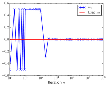
(a) Convergence of $m_{n}$

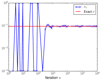
(b) Convergence of $\sigma_{n}$

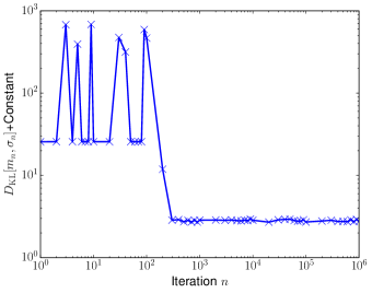
(c) Minimization of $D_{{\rm KL}}$

Fig. 1: Convergence of $m_{n}$ and $\sigma_{n}$ towards the values found via deterministic root finding for the scalar problem with potential (2.2) at $\varepsilon=0.01$. The iterates are generated using Algorithm 1, Robbins-Monro applied to KL minimization. Also plotted are values of KL divergence along the iteration sequence. The true optimal value is recovered, and KL divergence is reduced. To ensure convergence, $m_{n}$ is constrained to $[-.5,.5]$ and $\sigma_{n}$ is constrained to $[10^{-3},10^{0}]$.

2.2 Sampling of the Target Distribution

Having obtained values of $m$ and $\sigma$ that minimize $D_{{\rm KL}}(\nu\|\mu)$, we may use $\nu$ to develop an improved MCMC sampling algorithm for the target measure $\mu^{\varepsilon}$. We compare the performance of the standard pCN method of Algorithm 2, which uses no information about the best Gaussian fit $\nu$, with the improved pCN Algorithm 3, based on knowledge of $\nu.$ The improved performance, gauged by acceptance rate and autocovariance, is shown in Figure 2.

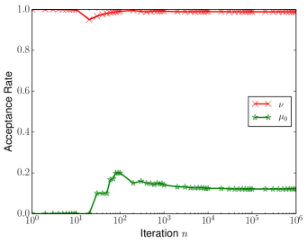
(a) Acceptance Rate

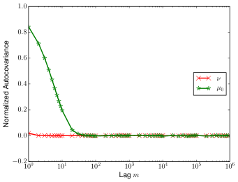
(b) Autocovariance

Fig. 2: Acceptance rates and autocovariances for sampling from (2.1) with potential (2.2) at $\varepsilon=0.01$. The curves labeled $\nu$ correspond to the samples generated using our improved MCMC, Algorithm 3, which uses the KL optimized $\nu$ for proposals. The curves labeled $\mu_{0}$ correspond to the samples generated using Algorithm 2, which relies on $\mu_{0}$ for proposals. Algorithm 3 shows an order of magnitude improvement over Algorithm 2. For clarity, only a subset of the data is plotted in the figures.

All of this is summarized by Figure 3, which shows the three distributions $\mu^{\varepsilon}$, $\mu_{0}$ and KL optimized $\nu$, together with a histogram generated by samples from the KL-optimized MCMC Algorithm 3. Clearly, $\nu$ better characterizes $\mu^{\varepsilon}$ than $\mu_{0}$, and this is reflected in the higher acceptance rate and reduced autocovariance. Though this is merely a scalar problem, these ideas are universal. In all of our examples, we have a non-Gaussian distribution we wish to sample from, an uninformed reference measure which gives poor sampling performance, and an optimized Gaussian which better captures the target measure and can be used to improve sampling.

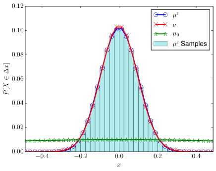
Fig. 3: Distributions of $\mu^{\varepsilon}$ (target), $\mu_{0}$ (reference) and $\nu$ (KL-optimized Gaussian) for the scalar problem with potential (2.2) at $\varepsilon=0.01$. Posterior samples have also been plotted, as a histogram. By inspection, $\nu$ better captures $\mu^{\varepsilon}$, leading to improved performance. $\Delta x=0.025$.

3 Parameterized Gaussian Approximations

We start in subsection 3.1 by describing some general features of the KL distance. Then in subsection 3.2 we discuss the case where $\nu$ is Gaussian. Subsections 3.3 and 3.4 describe two particular parameterizations of the Gaussian class that we have found useful in practice.

3.1 General Setting

Let $\nu$ be a measure defined by

$$\frac{d\nu}{d\mu_{0}}(u)=\frac{1}{Z_{\nu}}\exp\big{(}-\Phi_{\nu}(u)\big{)},$$ (3.1)

where we assume that $\Phi_{\nu}:X\to\mathbb{R}$ is continuous on $X.$ We aim to choose the best approximation $\nu$ to $\mu$ given by (1.1) from within some class of measures; this class will place restrictions on the form of $\Phi_{\nu}.$ Our best approximation is found by choosing the free parameters in $\nu$ to minimize the KL divergence between $\mu$ and $\nu$. This is defined as

$$D_{{\rm KL}}(\nu\|\mu)=\int_{H}\log\Bigl{(}\frac{d\nu}{d\mu}(u)\Bigr{)}\nu(du)=\mathbb{E}^{\nu}\log\Bigl{(}\frac{d\nu}{d\mu}(u)\Bigr{)}.$$ (3.2)

Recall that $D_{{\rm KL}}(\cdot\|\cdot)$ is not symmetric in its two arguments and our reason for choosing $D_{{\rm KL}}(\nu\|\mu)$ relates to the possibility of capturing multiple modes individually; minimizing $D_{{\rm KL}}(\mu\|\nu)$ corresponds to moment matching in the case where $\mathcal{A}$ is the set of all Gaussians [4, 24].

Provided $\mu_{0}\sim\nu$, we can write

$$\frac{d\mu}{d\nu}(u)=\frac{Z_{\nu}}{Z_{\mu}}\exp\bigl{(}-\Delta(u)\bigr{)},$$ (3.3)

where

$$\Delta(u)=\Phi_{\mu}(u)-\Phi_{\nu}(u).$$ (3.4)

Integrating this identity with respect to $\nu$ gives

$$\frac{Z_{\mu}}{Z_{\nu}}=\int_{H}\exp\bigl{(}-\Delta(u)\bigr{)}\nu(du)=\mathbb{E}^{\nu}\exp\bigl{(}-\Delta(u)\bigr{)}.$$ (3.5)

Combining (3.2) with (3.3) and (3.5), we have

$$D_{{\rm KL}}(\nu\|\mu)=\mathbb{E}^{\nu}\Delta(u)+\log\Bigl{(}\mathbb{E}^{\nu}\exp\bigl{(}-\Delta(u)\bigr{)}\Bigr{)}.$$ (3.6)

The computational task in this paper is to minimize (3.6) over the parameters that characterize our class of approximating measures $\mathcal{A}$, which for us will be subsets of Gaussians. These parameters enter $\Phi_{\nu}$ and the normalization constant $Z_{\nu}.$ It is noteworthy, however, that the normalization constants $Z_{\mu}$ and $Z_{\nu}$ do not enter this expression for the distance and are hence not explicitly needed in our algorithms.

To this end, it is useful to find the Euler-Lagrange equations of (3.6). Imagine that $\nu$ is parameterized by $\theta$ and that we wish to differentiate $J(\theta):=D_{{\rm KL}}(\nu\|\mu)$ with respect to $\theta.$ We rewrite $J(\theta)$ as an integral with respect to $\mu$, rather than $\nu$, differentiate under the integral, and then convert back to integrals with respect to $\nu.$ From (3.3), we obtain

$$\frac{Z_{\nu}}{Z_{\mu}}=\mathbb{E}^{\mu}e^{\Delta}.$$ (3.7)

Hence, from (3.3),

$$\frac{d\nu}{d\mu}(u)=\frac{e^{\Delta}}{\mathbb{E}^{\mu}e^{\Delta}}.$$ (3.8)

Thus we obtain, from (3.2),

$$J(\theta)=\mathbb{E}^{\mu}\Bigl{(}\frac{d\nu}{d\mu}(u)\log\Bigl{(}\frac{d\nu}{d\mu}(u)\Bigr{)}\Bigr{)}=\frac{\mathbb{E}^{\mu}\bigl{(}e^{\Delta}(\Delta-\log\mathbb{E}^{\mu}e^{\Delta})\bigr{)}}{\mathbb{E}^{\mu}e^{\Delta}},$$ (3.9)

and

$$J(\theta)=\frac{\mathbb{E}^{\mu}\bigl{(}e^{\Delta}\Delta\bigr{)}}{\mathbb{E}^{\mu}\bigl{(}e^{\Delta}\bigr{)}}-\log\mathbb{E}^{\mu}e^{\Delta}.$$

Therefore, with $D$ denoting differentiation with respect to $\theta$,

$$DJ(\theta)=\frac{\mathbb{E}^{\mu}\bigl{(}e^{\Delta}\Delta\,D\Delta\bigr{)}}{\mathbb{E}^{\mu}\bigl{(}e^{\Delta}\bigr{)}}-\frac{\mathbb{E}^{\mu}\bigl{(}e^{\Delta}\Delta\bigr{)}\mathbb{E}^{\mu}\bigl{(}e^{\Delta}D\Delta\bigr{)}}{\Bigl{(}\mathbb{E}^{\mu}\bigl{(}e^{\Delta}\bigr{)}\Bigr{)}^{2}}.$$

Using (3.8) we may rewrite this as integration with respect to $\nu$ and we obtain

$$DJ(\theta)=\mathbb{E}^{\nu}(\Delta\,D\Delta)-(\mathbb{E}^{\nu}\Delta)(\mathbb{E}^{\nu}D\Delta).$$ (3.10)

Thus, this derivative is zero if and only if $\Delta$ and $D\Delta$ are uncorrelated under $\nu.$

3.2 Gaussian Approximations

Recall that the reference measure $\mu_{0}$ is the Gaussian $N(m_{0},C_{0}).$ We assume that $C_{0}$ is a strictly positive-definite trace class operator on $\mathcal{H}$ [6]. We let $\{e_{j},\lambda_{j}^{2}\}_{j=1}^{\infty}$ denote the eigenfunction/eigenvalue pairs for $C_{0}$. Positive (resp. negative) fractional powers of $C_{0}$ are thus defined (resp. densely defined) on $\mathcal{H}$ by the spectral theorem and we may define $\mathcal{H}^{1}:=D(C_{0}^{-\frac{1}{2}})$, the Cameron-Martin space of measure $\mu_{0}$. We assume that $m_{0}\in\mathcal{H}^{1}$ so that $\mu_{0}$ is equivalent to $N(0,C_{0})$, by the Cameron-Martin Theorem [6]. We seek to approximate $\mu$ given in (1.1) by $\nu\in\mathcal{A}$, where $\mathcal{A}$ is a subset of the Gaussian measures on $\mathcal{H}$. It is shown in [24] that this implies that $\nu$ is equivalent to $\mu_{0}$ in the sense of measures and this in turn implies that $\nu=N(m,C)$ where $m\in E$ and

$$\Gamma:=C^{-1}-C_{0}^{-1}$$ (3.11)

satisfies

$$\big{\|}C_{0}^{\frac{1}{2}}\Gamma C_{0}^{\frac{1}{2}}\big{\|}_{\mathcal{HS}(\mathcal{H})}^{2}<\infty;$$ (3.12)

here $\mathcal{HS}(\mathcal{H})$ denotes the space of Hilbert-Schmidt operators on $\mathcal{H}$.

For practical reasons, we do not attempt to recover $\Gamma$ itself, but instead introduce low dimensional parameterizations. Two such parameterizations are introduced in this paper. In one, we introduce a finite rank operator, associated with a vector $\phi\in\mathbb{R}^{n}$. In the other, we employ a multiplication operator characterized by a potential function $b$. In both cases, the mean $m$ is an element of $\mathcal{H}^{1}$. Thus minimization will be over either $(m,\phi)$ or $(m,b)$.

In this Gaussian case the expressions for $D_{{\rm KL}}$ and its derivative, given by equations (3.6) and (3.10), can be simplified. Defining

$$\Phi_{\nu}(u)={-\langle u-m,m-m_{0}\rangle_{C_{0}}+\tfrac{1}{2}\langle u-m,\Gamma(u-m)\rangle-\tfrac{1}{2}\|m-m_{0}\|_{C_{0}}^{2}},$$ (3.13)

we observe that, assuming $\nu\sim\mu_{0}$,

$$\begin{split}\frac{d\nu}{d\mu_{0}}&\propto\exp\bigl{(}-\Phi_{\nu}(u)\bigr{)}.\end{split}$$ (3.14)

This may be substituted into the definition of $\Delta$ in (3.4), and used to calculate $J$ and $DJ$ according to (3.9) and (3.10). However, we may derive alternate expressions as follows. Let $\rho_{0}=N(0,C_{0})$, the centered version of $\mu_{0}$, and $\nu_{0}=M(0,C)$ the centered version of $\nu.$ Then, using the Cameron-Martin formula,

$$Z_{\nu}=\mathbb{E}^{\mu_{0}}\exp({-\Phi_{\nu}})=\mathbb{E}^{\rho_{0}}\exp({-\Phi_{\nu_{0}}})=\Bigl{(}\mathbb{E}^{\nu_{0}}\exp({\Phi_{\nu_{0}}})\Bigr{)}^{-1}=Z_{\nu_{0}},$$ (3.15)

where

$$\Phi_{\nu_{0}}=\tfrac{1}{2}\langle u,\Gamma u\rangle.$$ (3.16)

We also define a reduced $\Delta$ function which will play a role in our computations:

$$\Delta_{0}(u)\equiv{\Phi_{\mu}(u+m)-\tfrac{1}{2}\langle u,\Gamma u\rangle}.$$ (3.17)

The consequence of these calculations is that, in the Gaussian case, (3.6) is

$$\begin{split}D_{{\rm KL}}(\nu||\mu)&=\mathbb{E}^{\nu}\Delta-\log Z_{\nu_{0}}+\log Z_{\mu}\\ &=\mathbb{E}^{\nu_{0}}[\Delta_{0}]+\tfrac{1}{2}\|m-m_{0}\|_{C_{0}}^{2}+\log\mathbb{E}^{\nu_{0}}\exp(\tfrac{1}{2}\langle u,\Gamma u\rangle)+\log Z_{\mu}.\end{split}$$ (3.18)

Although the normalization constant $Z_{\mu}$ now enters the expression for the objective function, it is irrelevant in the minimization since it does not depend on the unknown parameters in $\nu$. To better see the connection between (3.6) and (3.18), note that

$$\frac{Z_{\mu}}{Z_{\nu_{0}}}=\frac{Z_{\mu}}{Z_{\nu}}=\frac{{\mathbb{E}}^{\mu_{0}}\exp(-\Phi_{\mu})}{{\mathbb{E}}^{\mu_{0}}\exp(-\Phi_{\nu})}={\mathbb{E}}^{\nu}\exp(-\Delta).$$ (3.19)

Working with (3.18), the Euler-Lagrange equations to be solved are:

$$D_{m}J(m,\theta) =\mathbb{E}^{\nu_{0}}D_{u}\Phi_{\mu}(u+m)+C_{0}^{-1}(m-m_{0}),$$ (3.20a)

$$D_{\theta}J(m,\theta) =\mathbb{E}^{\nu_{0}}(\Delta_{0}\,D_{\theta}\Delta_{0})-(\mathbb{E}^{\nu_{0}}\Delta_{0})(\mathbb{E}^{\nu_{0}}D_{\theta}\Delta_{0}).$$ (3.20b)

Here, $\theta$ is any of the parameters that define the covariance operator $C$ of the Gaussian $\nu$. Equation (3.20a) is obtained by direct differentiation of (3.18), while (3.20b) is obtained in the same way as (3.10). These expressions are simpler for computations for two reasons. First, for the variation in the mean, we do not need the full covariance expression of (3.10). Second, $\Delta_{0}$ has fewer terms to compute.

3.3 Finite Rank Parameterization

Let $P$ denote orthogonal projection onto $\mathcal{H}_{K}:=\operatorname{span}\{e_{1},\ldots,e_{K}\}$ the span of the first $K$ eigenvectors of $C_{0}$ and define $Q=I-P.$ We then parameterize the covariance $C$ of $\nu$ in the form

$$C^{-1}=\bigl{(}QC_{0}Q\bigr{)}^{-1}+\chi,\quad\chi=\sum_{i,j\leq K}\gamma_{ij}e_{i}\otimes e_{j}.$$ (3.21)

In words $C^{-1}$ is given by the inverse covariance $C_{0}^{-1}$ of $\mu_{0}$ on $Q\mathcal{H}$, and is given by $\chi$ on $P\mathcal{H}.$ Because $\chi$ is necessarily symmetric it is essentially parametrized by a vector $\phi$ of dimension $n=\frac{1}{2}K(K+1).$ We minimize $J(m,\phi):=D_{{\rm KL}}(\nu\|\mu)$ over $(m,\phi)\in\mathcal{H}^{1}\times\mathbb{R}^{n}.$ This is a well-defined minimization problem as demonstrated in Example 3.7 of [24] in the sense that minimizing sequences have weakly convergent subsequences in the admissible set. Minimizers need not be unique, and we should not expect them to be, as multimodality is to be expected, in general, for measures $\mu$ defined by (1.1).

3.4 Schrödinger Parameterization

In this subsection we assume that $\mathcal{H}$ comprises a Hilbert space of functions defined on a bounded open subset of $\mathbb{R}^{d}$. We then seek $\Gamma$ given by (3.11) in the form of a multiplication operator so that $(\Gamma u)(x)=b(x)u(x).$ Whilst minimization over the pair $(m,\Gamma)$, with $m\in\mathcal{H}^{1}$ and $\Gamma$ in the space of linear operators satisfying (3.12), is well-posed [24], minimizing sequences $\{m_{k},\Gamma_{k}\}_{k\geq 1}$ with $(\Gamma_{k}u)(x)=b_{k}(x)u(x)$ can behave very poorly with respect to the sequence $\{b_{k}\}_{k\geq 1}.$ For this reason we regularize the minimization problem and seek to minimize

$$J_{\alpha}(m,b)=J(m,b)+\tfrac{\alpha}{2}\|b\|_{r}^{2}$$

where $J(m,b):=D_{{\rm KL}}(\nu\|\mu)$ and $\|\cdot\|_{r}$ denotes the Sobolev space $H^{r}$ of functions on $\mathbb{R}^{d}$ with $r$ square integrable derivatives, with boundary conditions chosen appropriately for the problem at hand. The minimization of $J_{\alpha}(m,b)$ over $(m,b)\in\mathcal{H}\times H^{r}$ is well-defined; see Section 3.3 of [24].

4 Robbins-Monro Algorithm

In order to minimize $D_{{\rm KL}}(\nu\|\mu)$ we will use the Robbins-Monro algorithm [26, 2, 23, 20]. In its most general form this algorithm calculates zeros of functions defined via an expectation. We apply it to the Euler-Lagrange equations to find critical points of a non-negative objective function, defined via an expectation. This leads to a form of gradient descent in which we seek to integrate the equations

$$\dot{m}=-D_{m}D_{{\rm KL}},\quad\dot{\theta}=-D_{\theta}D_{{\rm KL}}$$

until they have reached a critical point. This requires two approximations. First, as (3.20) involve expectations, the right hand sides of these differential equations are evaluated only approximately, by sampling. Second, a time discretization must be introduced. The key idea underlying the algorithm is that, provided the step-length of the algorithm is sent to zero judiciously, the sampling error averages out and is diminished as the step length goes to zero.

4.1 Background on Robbins-Monro

In this section we review some of the structure in the Euler-Lagrange equations for the desired minimization of $D_{{\rm KL}}(\nu\|\mu)$. We then describe the particular variant of the Robbins-Monro algorithm that we use in practice. Suppose we have a parameterized distribution, $\nu_{\theta}$, from which we can generate samples, and we seek a value $\theta$ for which

$$f(\theta)\equiv{\mathbb{E}}^{\nu_{\theta}}[Y]=0,\quad Y\sim\nu_{\theta}.$$ (4.1)

Then an estimate of the zero, $\theta_{\star}$, can be obtained via the recursion

$$\theta_{n+1}=\theta_{n}-a_{n}\sum_{m=1}^{M}\tfrac{1}{M}Y_{m}^{(n)},\quad Y_{m}^{(n)}\sim\nu_{\theta_{n}},\quad\text{i.i.d.}$$ (4.2)

Note that the two approximations alluded to above are included in this procedure: sampling and (Euler) time-discretization. The methodology may be adapted to seek solutions to

$$f(\theta)\equiv{\mathbb{E}}^{\nu}[F(Y;\theta)]=0,\quad Y\sim\nu,$$ (4.3)

where $\nu$ is a given, fixed, distribution independent of the parameter $\theta$. (This setup arises, for example, in (3.20a), where $\nu_{0}$ is fixed and the parameter in question is $m.$) Letting $Z=F(Y;\theta)$, this induces a distribution $\eta_{\theta}(dz)=\nu(F^{-1}(dz;\theta))$, where the pre-image is with respect to the $Y$ argument. Then $f(\theta)={\mathbb{E}}^{\eta_{\theta}}[Z]$ with $Z\sim\eta_{\theta}$, and this now has the form of (4.1). As suggested in the extensive Robbins-Monro literature, we take the step sequence to satisfy

$$\sum_{n=1}^{\infty}a_{n}=\infty,\quad\sum_{n=1}^{\infty}a_{n}^{2}<\infty.$$ (4.4)

A suitable choice of $\{a_{n}\}$ is thus $a_{n}=a_{0}n^{-\gamma}$, $\gamma\in(1/2,1]$. The smaller the value of $\gamma$, the more “large” steps will be taken, helping the algorithm to explore the configuration space. On the other hand, once the sequence is near the root, the smaller $\gamma$ is, the larger the Markov chain variance will be. In addition to the choice of the sequence $a_{n}$, (4.1) introduces an additional parameter, $M$, the number of samples to be generated per iteration. See [7, 2] and references therein for commentary on sample size.

The conditions needed to ensure convergence, and what kind of convergence, have been relaxed significantly through the years. In their original paper, Robbins and Monro assumed that $Y\sim\mu_{\theta}$ were almost surely uniformly bounded, with a constant independent of $\theta$. If they also assumed that $f(\theta)$ was monotonic and $f^{\prime}(\theta_{\star})>0$, they could obtain convergence in $L^{2}$. With somewhat weaker assumptions, but still requiring that the zero be simple, Blum developed convergence with probability one, [5] . All of this was subsequently generalized to the arbitrary finite dimensional case; see [2, 20, 23].

As will be relevant to this work, there is the question of the applicability to the infinite dimensional case when we seek, for instance, a mean function in a separable Hilbert space. This has also been investigated; see [30, 10] along with references mentioned in the preface of [20]. In this work, we do not verify that our problems satisfy convergence criteria; this is a topic for future investigation.

A variation on the algorithm that is commonly applied is the enforcement of constraints which ensure $\{\theta_{n}\}$ remain in some bounded set; see [20] for an extensive discussion. We replace (4.2) by

$$\theta_{n+1}=\Pi_{D}\left[\theta_{n}-a_{n}\sum_{m=1}^{M}\tfrac{1}{M}Y_{m}^{(n)}\right],\quad Y_{m}^{(n)}\sim\nu_{\theta_{n}},\quad\text{i.i.d.},$$ (4.5)

where $D$ is a bounded set, and $\Pi_{D}(x)$ computes the point in $D$ nearest to $x$. This is important in our work, as the parameters that define must correspond to covariance operators. They must be positive definite, symmetric, and trace-class. Our method automatically produces symmetric trace-class operators, but the positivity has to be enforced by a projection.

4.2 Robbins-Monro Applied to KL

We seek minimizers of $D_{{\rm KL}}$ as stationary points of the associated Euler-Lagrange equations, (3.20). Before applying Robbins-Monro to this problem, we observe that we are free to precondition the Euler-Lagrange equations. In particular, we can apply bounded, positive, invertible operators so that pre-conditioned gradient will lie in the same function space as the parameter; this makes the iteration scheme well posed. For (3.20a), we have found pre-multiplying by $C_{0}$ to be sufficient. For (3.20b), the operator will be problem specific, depending on how $\theta$ parameterizes $C$, and also if there is a regularization. We denote the preconditioner for the second equation by $B_{\theta}$. Thus, the preconditioned Euler-Lagrange equations are

$$0= C_{0}\mathbb{E}^{\nu_{0}}D_{u}\Phi_{\mu}(u+m)+(m-m_{0}),$$ (4.6a)

$$0= B_{\theta}\left[\mathbb{E}^{\nu_{0}}(\Delta_{0}\,D_{\theta}\Delta_{0})-(\mathbb{E}^{\nu_{0}}\Delta_{0})(\mathbb{E}^{\nu_{0}}D_{\theta}\Delta_{0})\right].$$ (4.6b)

We must also ensure that $m$ and $\theta$ correspond to a well defined Gaussian; $C$ must be a covariance operator. Consequently, the Robbins-Monro iteration scheme is:

Algorithm 1.

1. Set $n=0$. Pick $m_{0}$ and $\theta_{0}$ in the admissible set, and choose a sequence $\{a_{n}\}$ satisfying (4.4)

2. Update $m_{n}$ and $\theta_{n}$ according to:

   $$m_{n+1} =\Pi_{m}\left[m_{n}-a_{n}\left\{C_{0}\left(\sum_{\ell=1}^{M}\tfrac{1}{M}\cdot D_{u}\Phi_{\mu}(u_{\ell})\right)+m_{n}-m_{0}\right\}\right],$$ (4.7a)

   $$\begin{split}\theta_{n+1}&=\Pi_{\theta}\left[\theta_{n}-a_{n}B_{\theta}\left\{\sum_{\ell=1}^{M}\tfrac{1}{M}\cdot\Delta_{0}(u_{\ell})D_{\theta}\Delta_{0}(u_{\ell})\right.\right.\\ &\hskip 56.9055pt\left.\left.-\left(\sum_{\ell=1}^{M}\tfrac{1}{M}\cdot\Delta_{0}(u_{\ell})\right)\left(\sum_{\ell=1}^{M}\tfrac{1}{M}\cdot D_{\theta}\Delta_{0}(u_{\ell})\right)\right\}\right].\end{split}$$ (4.7b)

3. $n\to n+1$ and return to 2

Typically, we have some a priori knowledge of the magnitude of the mean. For instance, $m\in H^{1}([0,1];\mathbb{R}^{1})$ may correspond to a mean path, joining two fixed endpoints, and we know it to be confined to some interval $[\underline{m},\overline{m}]$. In this case we choose

$$\Pi_{m}(f)(t)=\min\{\max\{f(t),\underline{m}\},\overline{m}\},\quad 0<t<1.$$ (4.8)

For $\Pi_{\theta}$, it is necessary to compute part of the spectrum of the operator that $\theta$ induces, check that it is positive, and if it is not, project the value to something satisfactory. In the case of the finite rank operators discussed in Section 3.3, the matrix $\boldsymbol{\gamma}$ must be positive. One way of handing this, for symmetric real matrices is to make the following choice:

$$\Pi_{\theta}(A)=X\mathop{\operator@font diag}\nolimits\{\min\{\max\{\boldsymbol{\lambda},\underline{\lambda}\},\overline{\lambda}\}\}X^{T},$$ (4.9)

where $A=X\mathop{\operator@font diag}\nolimits\{\boldsymbol{\lambda}\}X^{T}$ is the spectral decomposition, and $\underline{\lambda}$ and $\overline{\lambda}$ are constants chosen a priori. It can be shown that this projection gives the closest, with respect to the Frobenius norm, symmetric matrix with spectrum constrained to $[\underline{\lambda},\overline{\lambda}]$, [17].

5 Improved MCMC Sampling

The idea of the Metropolis-Hastings variant of MCMC is to create an ergodic Markov chain which is reversible, in the sense of Markov processes, with respect to the measure of interest; in particular the measure of interest is invariant under the Markov chain. In our case we are interested in the measure $\mu$ given by (1.1). Since this measure is defined on an infinite dimensional space it is advisable to use MCMC methods which are well-defined in the infinite dimensional setting, thereby ensuring that the resulting methods have mixing rates independent of the dimension of the finite dimensional approximation space. This philosophy is explained in the paper [9]. The pCN algorithm is perhaps the simplest MCMC method for (1.1) meeting these requirements. It has the following form:

Algorithm 2.

Define $a_{\mu}(u,v):=\min\{1,\exp\bigl{(}\Phi_{\mu}(u)-\Phi_{\mu}(v)\bigr{)}\}.$

1. Set $k=0$ and Pick $u^{(0)}$

2. $v^{(k)}=m_{0}+\sqrt{(1-\beta^{2})}(u^{(k)}-m_{0})+\beta\xi^{(k)},\quad\xi^{(k)}\sim N(0,C_{0})$

3. Set $u^{(k+1)}=v^{(k)}$ with probability $a_{\mu}(u^{(k)},v^{(k)})$

4. Set $u^{(k+1)}=u^{(k)}$ otherwise

5. $k\to k+1$ and return to 2

This algorithm has a spectral gap which is independent of the dimension of the discretization space under quite general assumptions on $\Phi_{\mu}$ [15]. However, it can still behave poorly if $\Phi_{\mu}$, or its gradients, are large. This leads to poor acceptance probabilities unless $\beta$ is chosen very small so that proposed moves are localized; either way, the correlation decay is slow and mixing is poor in such situations. This problem arises because the underlying Gaussian $\mu_{0}$ used in the algorithm construction is far from the target measure $\mu$. This suggests a potential resolution in cases where we have a good Gaussian approximation to $\mu$, such as the measure $\nu$. Rather than basing the pCN approximation on (1.1) we base it on (3.3); this leads to the following algorithm:

Algorithm 3.

Define $a_{\nu}(u,v):=\min\{1,\exp\bigl{(}\Delta(u)-\Delta(v)\bigr{)}\}.$

1. Set $k=0$ and Pick $u^{(0)}$

2. $v^{(k)}=m+\sqrt{(1-\beta^{2})}(u^{(k)}-m)+\beta\xi^{(k)},\quad\xi^{(k)}\sim N(0,C)$

3. Set $u^{(k+1)}=v^{(k)}$ with probability $a_{\nu}(u^{(k)},v^{(k)})$

4. Set $u^{(k+1)}=u^{(k)}$ otherwise

5. $k\to k+1$ and return to 2

We expect $\Delta$ to be smaller than $\Phi$, at least in regions of high $\mu$ probability. This suggests that, for given $\beta$, Algorithm 3 will have better acceptance probability than Algorithm 2, leading to more rapid sampling. We show in what follows that this is indeed the case.

6 Numerical Results

In this section we describe our numerical results. These concern both solution of the relevant minimization problem, to find the best Gaussian approximation from within a given class using Algorithm 1 applied to the two parameterizations given in subsections 3.3 and 3.4, together with results illustrating the new pCN Algorithm 3 which employs the best Gaussian approximation within MCMC. We consider two model problems: a Bayesian Inverse problem arising in PDEs, and a Conditioned Diffusion problem motivated by molecular dynamics. Some details on the path generation algorithms used in these two problems are given in Appendix B.

6.1 Bayesian Inverse Problem

We consider an inverse problem arising in groundwater flow. The forward problem is modelled by the Darcy constitutive model for porous medium flow. The objective is to find $p\in V:=H^{1}$ given by the equation

$$-\nabla\cdot\bigl{(}\exp(u)\nabla p\bigr{)} =0,\quad x\in D,$$ (6.1a)

$$p =g,\quad x\in\partial D.$$ (6.1b)

The inverse problem is to find $u\in X=L^{\infty}(D)$ given noisy observations

$$y_{j}=\ell_{j}(p)+\eta_{j},$$

where $\ell_{j}\in V^{*}$, the space of continuous linear functionals on $V$. This corresponds to determining the log permeability from measurements of the hydraulic head (height of the water-table). Letting $\mathcal{G}(u)={\ell}(p(\cdot;u))$, the solution operator of (6.1) composed with the vector of linear functionals ${\ell}=(\ell_{j})^{T}$. We then write, in vector form,

$$y=\mathcal{G}(u)+\eta.$$

We assume that $\eta\sim N(0,\Sigma)$ and place a Gaussian prior $N(m_{0},C_{0})$ on $u$. Then the Bayesian inverse problem has the form (1.1) where

$$\Phi(u):=\frac{1}{2}\bigl{\|}\Sigma^{-\frac{1}{2}}\bigl{(}y-\mathcal{G}(u)\bigr{)}\bigr{\|}^{2}.$$

We consider this problem in dimension one, with $\Sigma=\gamma^{2}I$, and employing pointwise observation at points $x_{j}$ as the linear functionals $\ell_{j}$. As prior we take the Gaussian $\mu_{0}=N(0,C_{0})$, with

$$C_{0}=\delta\left(-\frac{d^{2}}{dx^{2}}\right)^{-1},$$

restricted to the subspace of $L^{2}(0,1)$ of periodic mean zero functions. In one dimension we may solve the forward problem (6.1) on $D=(0,1)$, with $p(0)=p^{-}$ and $p(1)=p^{+}$ explicitly to obtain

$$p(x;u)=(p^{+}-p^{-})\frac{J_{x}(u)}{J_{1}(u)}+p^{-},\quad J_{x}(u)\equiv\int_{0}^{x}\exp(-u(z))dz,$$ (6.2)

and

$$\Phi(u)=\frac{1}{2\gamma^{2}}\sum_{j=1}^{\ell}|p(x_{j};u)-y_{j}|^{2}$$ (6.3)

Following the methodology of [18], to compute $D_{u}\Phi(u)$, we must solve the adjoint problem for $q$:

$$-\frac{d}{dx}\left(\exp(u)\frac{dq}{dx}\right)=-\frac{1}{\gamma^{2}}\sum_{j=1}^{\ell}(p(x_{j};u)-y_{j})\delta_{x_{j}},\quad q(0)=q(1)=0.$$ (6.4)

Again, we can write the solution explicitly via quadrature:

$$\begin{split}q(x;u)&=K_{x}(u)-\frac{K_{1}(u)J_{x}(u)}{J_{1}(u)},\\ K_{x}(u)&\equiv\sum_{j=1}^{\ell}\frac{p(x_{j};u)-y_{j}}{\gamma^{2}}\int_{0}^{x}\exp(-u(z))H(z-x_{j})dz\end{split}$$ (6.5)

Using (6.2) and (6.5),

$$D_{u}\Phi(u)=\exp(u)\frac{dp(x;u)}{dx}\frac{dq(x;u)}{dx}.$$ (6.6)

For this application we use a finite rank approximation of the covariance of the approximating measure $\nu$, as explained in subsection 3.3. In computing with the finite rank matrix (3.21), it is useful, for good convergence, to work with $B=\boldsymbol{\gamma}^{-1/2}$. The preconditioned derivatives, (4.6), also require $D_{B}\Delta_{0}$, where $\Delta_{0}$ is given by (3.17). To characterize this term, if $v=\sum_{i}v_{i}e_{i}$, we let ${\bf v}=(v_{1},\ldots v_{N})^{T}$ be the first $N$ coefficients. Then for the finite rank approximation,

$$\Phi_{\nu_{0}}(v)=\frac{1}{2}\left\langle v,(C^{-1}-C_{0}^{-1})v\right\rangle=\frac{1}{2}{\bf v}^{T}(\boldsymbol{\gamma}-\mathop{\operator@font diag}\nolimits(\lambda_{1}^{-1},\ldots\lambda_{N}^{-1})){\bf v}.$$ (6.7)

Then using our parameterization with respect to the matrix $B$,

$$D_{B}\Delta_{0}(v)=D_{B}(\Phi(m+v)-\Phi_{\nu_{0}}(v))=\frac{1}{2}\left[B^{-1}{\bf v}(B^{-2}{\bf v})^{T}+B^{-2}{\bf v}(B^{-1}{\bf v})^{T}\right].$$ (6.8)

As a preconditioner for (4.6b) we found that it was sufficient to multiply by $\lambda_{N}$.

We solve this problem with Ranks $K=$ 2, 4, 6, first minimizing $D_{{\rm KL}}$, and then running the pCN Algorithm 3 to sample from $\mu_{y}$. The common parameters are:

• $\gamma=0.1$, $\delta=1$, $p^{-}=0$ and $p^{+}=2$;

• There are $2^{7}$ uniformly spaced grid points in $[0,1)$;

• (6.2) and (6.5) are solved via trapezoidal rule quadrature;

• The true value of $u(x)=2\sin(2\pi x)$;

• The dimension of the data is four, with samples at $x=0.2,0.4,0.6,0.8$;

• $m_{0}=0$ and $B_{0}=\mathop{\operator@font diag}\nolimits(\lambda_{n})$, $n\leq\text{Rank}$;

• $\int\dot{m}^{2}$ is estimated spectrally;

• $10^{5}$ iterations of the Robbins-Monro algorithm are performed with $10^{2}$ samples per iteration;

• $a_{0}=.1$ and $a_{n}=a_{0}n^{-3/5}$;

• The eigenvalues of $\sigma$ are constrained to the interval $[10^{-4},10^{0}]$ and the mean is constrained to $[-5,5]$;

• pCN Algorithms 2 and 3 are implemented with $\beta=0.6$, and $10^{6}$ iterations.

The results of the $D_{{\rm KL}}$ optimization phase of the problem, using the Robbins-Monro Algorithm 1, appear in Figure 4. This figure shows: the convergence of $m_{n}$ in the Rank 2 case; the convergence of the eigenvalues of $B$ for Ranks 2, 4, and 6; and the minimization of $D_{{\rm KL}}$. We only present the convergence of the mean in the Rank 2 case, as the others are quite similar. At the termination of the Robbins-Monro step, the $B_{n}$ matrices are:

$${B}_{n} =\begin{pmatrix}0.0857&0.00632\\ -&0.105\end{pmatrix}$$ (6.9)

$${B}_{n} =\begin{pmatrix}0.0864&0.00500&-0.00791&-0.00485\\ -&0.106&0.00449&-0.00136\\ -&-&0.0699&-0.000465\\ -&-&-&0.0739\end{pmatrix}$$ (6.10)

$${B}_{n} =\begin{pmatrix}0.0870&0.00518&-0.00782&-0.00500&-0.00179&-0.00142\\ -&0.106&0.00446&-0.00135&0.00107&0.00166\\ -&-&0.0701&-0.000453&-0.00244&9.81\times 10^{-5}\\ -&-&-&0.0740&-0.00160&0.00120\\ -&-&-&-&0.0519&-0.00134\\ -&-&-&-&-&0.0523\end{pmatrix}$$ (6.11)

Note there is consistency as the rank increases, and this is reflected in the eigenvalues of the $B_{n}$ shown in Figure 4. As in the case of the scalar problem, more iterations of Robbins-Monro are computed than are needed to ensure convergence.

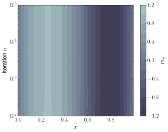
(a) Convergence of $m_{n}(x)$ for Rank 2

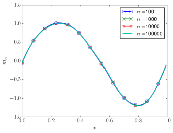
(b) $m_{n}(x)$ for Rank 2 at Particular Iterations

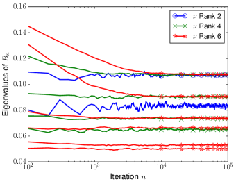
(c) Convergence of the eigenvalues of $B_{n}$

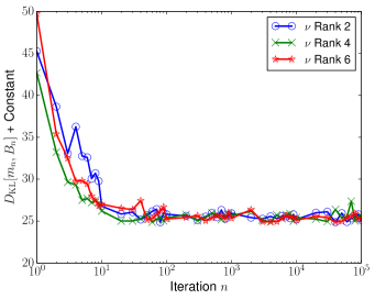
(d) Minimization of $D_{{\rm KL}}$

Fig. 4: Convergence of the Robbins-Monro Algorithm 1 applied to the Bayesian Inverse problem. Figures (a) and (b) show the convergence of $m_{n}$ in the case of Rank 2, while Figure (c) shows the convergence of the eigenvalues of $B_{n}$ for Ranks 2, 4 and 6. Figure (d) shows the minimization of $D_{{\rm KL}}$. The observational noise is $\gamma=0.1$. The figures indicate that Rank 2 has converged after $10^{2}$ iterations; Rank 4 has converged after $10^{3}$ iterations; and Rank 6 has converged after $10^{4}$ iterations.

The posterior sampling, by means of Algorithms 2 and 3, is described in Figure 5. There is good posterior agreement in the means and variances in all cases, and the low rank priors provide not just good means but also variances. This is reflected in the high acceptance rates and low auto covariances; there is approximately an order of magnitude in improvement in using Algorithm 3, which is informed by the best Gaussian approximation, and Algorithm 2, which is not.

However, notice in Figure 4 that the posterior, even when $\pm$ one standard deviation is included, does not capture the truth. The results are more favorable when we consider the pressure field, and this hints at the origin of the disagreement. The values at $x=0.2$ and 0.4, and to a lesser extent at 0.6, are dominated by the noise. Our posterior estimates reflect the limitations of what we are able to predict given our assumptions. If we repeat the experiment with smaller observational noise, $\gamma=0.01$ instead of $0.1$, we see better agreement, and also variation in performance with respect to approximations of different ranks. These results appear in Figure 6. In this smaller noise case, there is a two order magnitude improvement in performance.

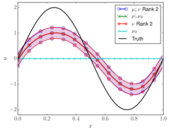
(a) Log permeability $u(x)$

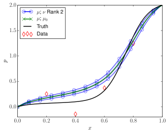
(b) Pressure $p(x)$

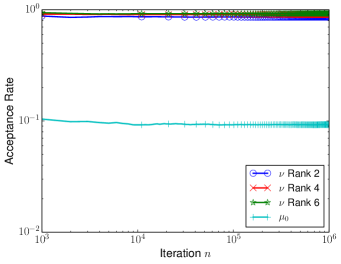
(c) Acceptance Rate

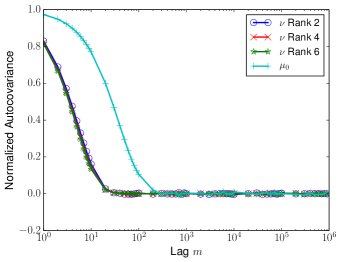
(d) Autocovariance

Fig. 5: Behavior of MCMC Algorithms 2 and 3 for the Bayesian Inverse problem with observational noise $\gamma=0.1$. The true posterior distribution, $\mu$, is sampled using $\mu_{0}$ (Algorithm 2) and $\nu$, with Ranks 2, 4 and 6 (Algorithm 3). The resulting posterior approximations are labeled $\mu;\;\mu_{0}$ (Algorithm 2) and $\mu;\;\nu$ Rank 2, (Algorithm 3). The notation $\mu_{0}$ and $\nu$ Rank $K$ is used for the prior and best Gaussian approximations of the corresponding rank. The distributions of $u(x)$, in Figure (a), for the optimized $\nu$ Rank 2 and the posterior $\mu$ overlap, but are still far from the truth. The results for Ranks 4 and 6 are similar. Figures (c) and (d) compare the performance of Algorithm 3 when using $\nu$ Rank K for the proposal, with $K=$2, 4, and 6, against Algorithm 2. $\nu$ Rank 2 gives an order of magnitude improvement in posterior sampling over $\mu_{0}$. There is not significant improvement when using $\nu$ Ranks 4 and 6 over using Rank 2. Shaded regions enclose $\pm$ one standard deviation.

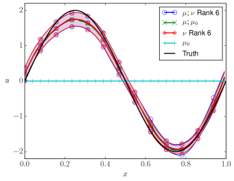
(a) Log permeability $u(x)$

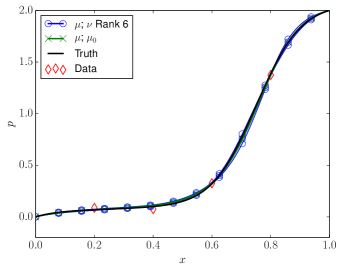
(b) Pressure $p(x)$

(c) Acceptance Rate

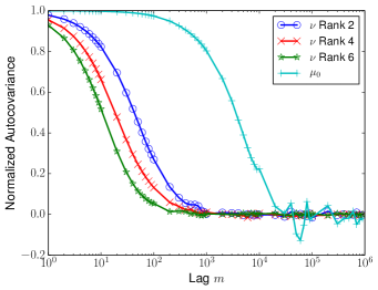
(d) Autocovariance

Fig. 6: Behavior of MCMC Algorithms 2 and 3 for the Bayesian Inverse problem with observational noise $\gamma=0.01$. Notation as in Figure 5. The distribution of $u(x)$, shown in Figure (a), for both the optimized Rank 6 $\nu$, and the posterior $\mu$ overlap, and are close to the truth. Unlike the case of $\gamma=0.1$, Figures (c) and (d) show improvement in using $\nu$ Rank 6 within Algorithm 3, over Ranks 2 and 4. However, all three cases of Algorithm 3 are at least two orders of magnitude better than Algorithm 2, which uses only $\mu_{0}$. Shaded regions enclose $\pm$ one standard deviation.

6.2 Conditioned Diffusion Process

Next, we consider measure $\mu$ given by (1.1) in the case where $\mu_{0}$ is a unit Brownian bridge connecting $0$ to $1$ on the interval $(0,1)$, and

$$\Phi=\frac{1}{4\varepsilon^{2}}\int_{0}^{1}\Bigl{(}1-u(t)^{2}\Bigr{)}^{2}dt,$$

a double well potential. This also has an interpretation as a conditioned diffusion [25]. Note that $m_{0}=t$ and $C_{0}^{-1}=-\tfrac{1}{2}\tfrac{d^{2}}{dt^{2}}$ with $D(C_{0}^{-1})=H^{2}(I)\cap H^{1}_{0}(I)$ with $I=(0,1).$

We seek the approximating measure $\nu$ in the form $N(m(t),C)$ with $(m,B)$ to be varied, where

$$C^{-1}=C_{0}^{-1}+\tfrac{1}{2\varepsilon^{2}}B$$

and $B$ is either constant,$B\in\mathbb{R}$, or $B:I\to\mathbb{R}$ is a function viewed as a multiplication operator.

We examine both cases of this problem, performing the optimization, followed by pCN sampling. The results were then compared against the uninformed prior, $\mu_{0}=N(m_{0},C_{0})$. For the constant $B$ case, no preconditioning on $B$ was performed, and the initial guess was $B=1$. For $B=B(t)$, a Tikhonov-Phillips regularization was introduced,

$$D_{{\rm KL}}^{\alpha}=D_{{\rm KL}}+\frac{\alpha}{2}\int\dot{B}^{2}dt,\quad\alpha=10^{-2}.$$ (6.12)

For computing the gradients (4.6) and estimating $D_{{\rm KL}}$,

$$D_{m}\Phi(v+m) =\tfrac{1}{2\varepsilon^{2}}(v+m)[(v+m)^{2}-1],$$ (6.13a)

$$D_{B}\Phi_{\nu_{0}}(v) =\begin{cases}\frac{1}{4\varepsilon^{2}}\int_{0}^{1}v^{2}dt&\text{$B$ constant}\\ \frac{1}{4\varepsilon^{2}}v^{2}&\text{$B(t)$}\end{cases}.$$ (6.13b)

No preconditioning is applied for (6.13b) in the case that $B$ is a constant, while in the case that $B(t)$ is variable, the preconditioned gradient in $B$ is

$$\left\{-\alpha\tfrac{d^{2}}{dt^{2}}\right\}^{-1}\left({\mathbb{E}}^{\nu_{0}}(\Delta_{0}D_{\theta}\Delta_{0})-{\mathbb{E}}^{\nu_{0}}(\Delta_{0}){\mathbb{E}}^{\nu_{0}}(D_{\theta}\Delta_{0})\right)+B.$$

Because of the regularization, we must invert $-d^{2}/dt^{2}$, requiring the specification of boundary conditions. By a symmetry argument, we specify the Neumann boundary condition, $B^{\prime}(0)=0$. At the other endpoint, we specify the Dirichlet condition $B(1)=V^{\prime\prime}(1)=2$, a “far field” approximation.

The common parameters used are:

• The temperature $\varepsilon=0.05$;

• There were $99$ uniformly spaced grid points in $(0,1)$;

• As the endpoints of the mean path are 0 and 1, we constrained our paths to lie in $[0,1.5]$;

• $B$ and $B(t)$ were constrained to lie in $[10^{-3},10^{1}]$, to ensure positivity of the spectrum;

• The standard second order centered finite difference scheme was used for $C_{0}^{-1}$;

• Trapezoidal rule quadrature was used to estimate $\int_{0}^{1}\dot{m}^{2}$ and $\int_{0}^{1}\dot{B}^{2}dt$, with second order centered differences used to estimate the derivatives;

• $m_{0}(t)=t$, $B_{0}=1$, $B_{0}(t)=V^{\prime\prime}(1)$, the right endpoint value;

• $10^{5}$ iterations of the Robbins-Monro algorithm are performed with $10^{2}$ samples per iteration;

• $a_{0}=2$ and $a_{n}=a_{0}n^{-3/5}$;

• pCN Algorithms 2 and 3 are implemented with $\beta=0.6$, and $10^{6}$ iterations.

Our results are favorable, and the outcome of the Robbins-Monro Algorithm 1 is shown in Figures 7 and 8 for the additive potentials $B$ and $B(t)$, respectively. The means and potentials converge in both the constant and variable cases. Figure 9 confirms that in both cases, $D_{{\rm KL}}$ and $D_{{\rm KL}}^{\alpha}$ are reduced during the algorithm.

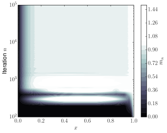
(a) $m_{n}(t)$ versus $n$.

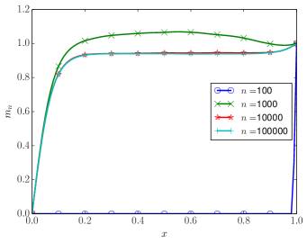
(b) $m_{n}(t)$ at Particular Iterations

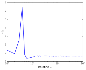
(c) $B_{n}$ versus $n$.

Fig. 7: Convergence of the Robbins-Monro Algorithm 1 applied to the Conditioned Diffusion problem, in the case of constant inverse covariance potential $B$. Figure (a) shows evolution of $m_{n}(t)$ with $n$; Figure (b) shows $m_{n}(t)$ at particular $n$. Figure (c) shows convergence of the $B_{n}$ constant.

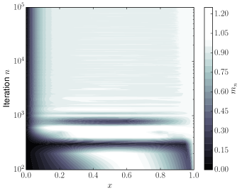
(a) $m_{n}(t)$ versus $n$.

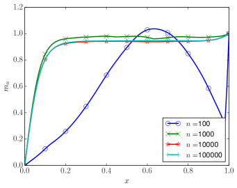
(b) $m_{n}(t)$ at Particular Iterations.

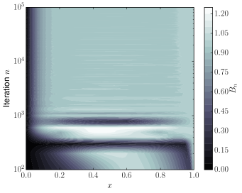
(c) $B_{n}(t)$ versus $n$.

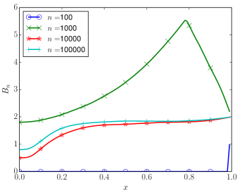
(d) $B_{n}(t)$ at Particular Iterations.

Fig. 8: Convergence of the Robbins-Monro Algorithm 1 applied to the Conditioned Diffusion problem, in the case of variable inverse covariance potential $B(t)$. Figure (a) shows evolution of $m_{n}(t)$ with $n$; Figure (b) shows $m_{n}(t)$ at particular $n$. Figure (c) shows evolution of $B_{n}(t)$ with $n$; Figure (d) shows $B_{n}(t)$ at particular $n$.

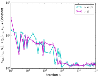
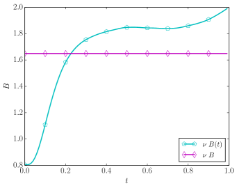
Fig. 9: Minimization of $D_{{\rm KL}}^{\alpha}$ (for $B(t)$) and $D_{{\rm KL}}$ (for $B$) during Robbins-Monro Algorithm 1 for the Conditioned Diffusion problem. Also plotted is a comparison of $B$ and $B(t)$ for the optimized $\nu$ distributions.

The important comparison is when we sample the posterior using these as the proposal distributions in MCMC Algorithms 2 and 3. The results for this are given in Figure 10. Here, we compare both the prior and posterior means and variances, along with the acceptance rates. The means are all in reasonable agreement, with the exception of the $m_{0}$, which was to be expected. The variances indicate that the sampling done using $\mu_{0}$ has not quite converged, which is why it is far from the posterior variances obtained from the optimized $\nu$’s, which are quite close. The optimized prior variances recover the plateau between $t=0.2$ to $t=0.9$, but could not resolve the peak near $0.1$. Variable $B(t)$ captures some of this information in that it has a maximum in the right location, but of a smaller amplitude. However, when one standard deviation about the mean is plotted, it is difficult to see this disagreement in variance between the reference and target measures.

In Figure 11 we present the acceptance rate and autocovariance, to assess the performance of Algorithms 2 and 3. For both the constant and variable potential cases, there is better than an order of magnitude improvement over $\mu_{0}$. In this case, it is difficult to distinguish an appreciable difference in performance between $B(t)$ and $B$.

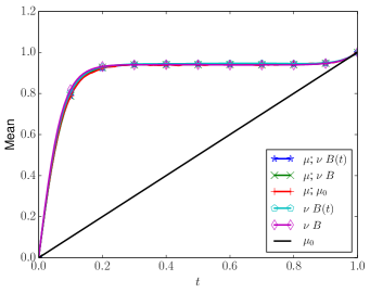
(a) Mean

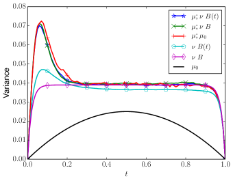
(b) Variance

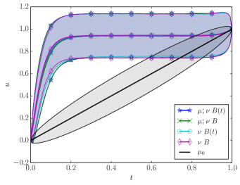
(c) $u(t$)

Fig. 10: Behavior of MCMC Algorithms 2 and 3 for the Conditioned Diffusion problem. The true posterior distribution, $\mu$, is sampled using $\mu_{0}$ (Algorithm 2) and $\nu$, for both constant and variable potentials, $B$ and $B(t)$, (Algorithm 3). The resulting posterior approximations are denoted by $\mu;\mu_{0}$ (Algorithm 2), and $\mu;\nu B$ and $\mu;\nu B(t)$ (Algorithm 3). The curves denoted $\mu_{0}$, and $\nu\;B$ and $\nu\;B(t)$, are the prior and best fit Gaussians. For both optimized $\nu$’s, there is good agreement between the means and the posterior mean. The variances are consistent, but the posterior shows a peak near $t=0.1$ that is not captured by $\nu$ distributions. With the exception of $\mu_{0}$, there is good general agreement amongst the distributions of $u(t)$. Shaded regions enclose $\pm$ one standard deviation.

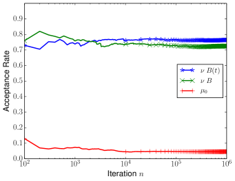
(a) Acceptance Rate

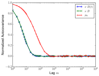
(b) Autocovariance

Fig. 11: Performance of MCMC Algorithms 2 and 3 for the Conditioned Diffusion problem. When $\mu_{0}$ is used for proposals in Algorithm 2, the acceptance rate is far beneath either best fit Gaussian, $\nu\;B$ and $\nu\;B(t)$, within Algorithm 3. Variable $B(t)$ provides nominal improvement over constant $B$.

7 Conclusions

We have demonstrated a viable computational methodology for finding the best Gaussian approximation to measures defined on a Hilbert space of functions, using the Kullback-Leibler divergence as measure of fit. We have parameterized the covariance via low rank matrices, or via a Schrödinger potential in an inverse covariance representation, and represented the mean nonparametrically, as a function; these representations are guided by knowledge and understanding of the properties of the underlying calculus of variations problem as described in [24]. Computational results demonstrate that, in certain natural parameter regimes, the Gaussian approximations are good in the sense that they give estimates of mean and covariance which are close to the true mean and covariance under the target measure of interest, and that they consequently can be used to construct efficient MCMC methods to probe the posterior distribution.

Further work is needed to explore the methodology in larger scale applications and to develop application-specific parameterizations of the covariance in this context. It would also be interesting to combine the Robbins-Monro minimization with the MCMC method to construct an adaptive MCMC method. On the analysis side it would be instructive to demonstrate improved spectral gaps for the resulting MCMC methods, with respect to observational noise (resp. temperature) within the context of Bayesian inverse problems (resp. conditioned diffusions), generalizing the analysis of Section 2.

Appendix A Scalar Example

In this section of the appendix we provide further details relating to the motivational scalar example from section 2.

A.1 Scalar Sampling

Recall the scalar problem from Section 2. One of the motivations for considering such a problem is that many of the calculations for $D_{{\rm KL}}(\nu\|\mu)$ are explicit. Indeed, If $\nu=N(m,\sigma^{2})$ is the Gaussian which we intend to fit against $\mu$, then

$$\begin{split}D_{{\rm KL}}(\nu||\mu)&={\mathbb{E}}^{\nu}\left[V(x)-\tfrac{1}{2\sigma^{2}}|x-m|^{2}\right]+\log Z_{\mu}-\log Z_{\nu}\\ &={\mathbb{E}}^{\nu_{0}}[V(y+m)]-\tfrac{1}{2}+\log Z_{\mu}-\log\sigma-\log\sqrt{2\pi},\\ &={\mathbb{E}}^{\nu_{0}}[V(y+m)]-\log\sigma+\text{Constant}.\end{split}$$ (A.1)

The derivatives then take the simplified form

$$D_{m}D_{{\rm KL}} ={\mathbb{E}}^{\nu_{0}}[D_{y}V(y+m)],$$ (A.2a)

$$D_{\sigma}D_{{\rm KL}} ={\mathbb{E}}^{\nu_{0}}[V(y+m)\sigma^{-3}(y^{2}-\sigma^{2})]-\sigma^{-1}.$$ (A.2b)

For some choices of $V(x)$, including (2.2), the above expectations can be computed analytically, and the critical points of (A.2) can then be obtained by classical root finding. Thus, we will be able to compare the Robbins-Monro solution against a deterministic one, making for an excellent benchmark problem.

The parameters used in these computation are:

• $10^{6}$ iterations of the Robbins-Monro with $10^{2}$ samples per iterations;

• $a_{0}=.1$ and $a_{n}=a_{0}n^{-3/5}$;

• $m_{0}=0$ and $\sigma_{0}=1$;

• $m$ is constrained to the interval $[-.5,.5]$;

• $\sigma$ is constrained to the interval $[10^{-3},10^{0}]$;

• $10^{6}$ iterations of pCN, Algorithms 2, 3, are performed with $\beta=1.$

While $10^{6}$ iterations of Robbins-Monro are used, Figure 1 indicates that there is good agreement after $10^{3}$ iterations. More iterations than needed are used in all of our examples, to ensure convergence. With appropriate convergence diagnostics, it may be possible to identify a convenient termination time.

A.2 Analysis of the Sampling Performance

While the numerical experiments confirm our intuition, for this example, the acceptance rate can be studied analytically. Let

$$T(u,v)=\tfrac{1}{\varepsilon}(u^{4}-v^{4})+\left(\tfrac{1}{2\varepsilon}-\tfrac{1}{2\sigma^{2}}\right)(u^{2}-v^{2})+\tfrac{m}{\sigma^{2}}(u-v).$$ (A.3)

The acceptance probability for proposal $v$, given current state $u$, is then $1\wedge e^{T}$. This is valid not only for our new Algorithm 3, using the optimized distribution $\nu=N(m,\sigma^{2})$, but also for Algorithm 2, which uses the prior $\mu_{0}$, by taking $m\mapsto 0$ and $\sigma\mapsto 1$ in (A.3).

For an independence sampler, where proposals are generated solely from $\nu$, we show that the expected acceptance rate of the optimized $\nu$ tends to one as $\varepsilon\to 0$. In contrast, when the prior, $\mu_{0}=N(0,1)$ is used as the proposal distribution, the acceptance rate will be driven to zero. We emphasize this case as the independence sampler should have the poorest acceptance rate. If instead of using an independence sampler, we use a Crank-Nicolson proposal with sufficiently small steps, favorable acceptance rates can be recovered when $\mu_{0}$ is used for proposals.

These results are partially based on the following lemma, which provides a lower bound on the acceptance rate:

Lemma 4 (Lemma B.1 of [3]).

Let $Y$ be a real-valued random variable and $\gamma>0$. Then

$${\mathbb{E}}[1\wedge e^{Y}]\geq e^{-\gamma}\left(1-\gamma^{-1}{{\mathbb{E}}[|Y|]}\right).$$

Proposition 5.

Assume $\nu$ is the $D_{{\rm KL}}$ optimized distribution for (2.1) with potential (2.2). Furthermore, assume that $\mu^{\varepsilon}$ is sampled using Algorithm 3 with $\beta=1$, and that it has reached stationarity. Then ${\mathbb{E}}[|T|]\leq 18\varepsilon+\operatorname{O}(\varepsilon^{2})$, and for any fixed $\gamma>0$, $\lim_{\varepsilon\to 0}{\mathbb{E}}[1\wedge e^{T}]\geq e^{-\gamma}$.

Proof.

First we estimate ${\mathbb{E}}[|T|]$, then we apply Lemma 4. Since we are considering the case of the independence sampler, and have reached stationarity, we may take $u\sim\mu^{\varepsilon}$ and $v\sim\nu$ to be independent. Then, taking $m=0$ and $\sigma^{2}$ given by (2.5),

$$\begin{split}{\mathbb{E}}[|T|]&\leq{\mathbb{E}}^{\mu^{\varepsilon}}\left[\tfrac{1}{\varepsilon}u^{4}+(6+\operatorname{O}(\varepsilon))u^{2}\right]+{\mathbb{E}}^{\nu}\left[\tfrac{1}{\varepsilon}v^{4}+(6+\operatorname{O}(\varepsilon))v^{2}\right]\\ &\leq 3\varepsilon+6\varepsilon+3\varepsilon+6\varepsilon+\operatorname{O}(\varepsilon^{2}).\end{split}$$

Details of the moment estimates are given in Section A.3. The result is now obvious. ∎

Proposition 6.

Assume that $\mu^{\varepsilon}$ is sampled using Algorithm 2 with $\beta=1$, and that it has reached stationarity. Then ${\mathbb{E}}[1\wedge e^{T}]\lesssim\varepsilon^{1/2}$.

Proof.

The strategy is to make estimates using a Gaussian in place of $\mu^{\varepsilon}$. Let $\tilde{\mu}^{\varepsilon}=N(0,\varepsilon)$, and when denote $\tilde{u}\sim\tilde{\mu}^{\varepsilon}$ to distinguish it form $\mu^{\varepsilon}$. Then, since $1\wedge e^{T}\geq 0$,

$${\mathbb{E}}[1\wedge e^{T}]={\mathbb{E}}[1\wedge e^{T(u,v)}]\leq\frac{\sqrt{2\pi\varepsilon}}{Z_{\varepsilon}}{\mathbb{E}}[1\wedge e^{T(\tilde{u},v)}]=(1+\operatorname{O}(\varepsilon)){\mathbb{E}}[1\wedge e^{T(\tilde{u},v)}].$$

The estimate of $Z_{\varepsilon}$ is given in Section A.3, and

$${\mathbb{E}}[1\wedge e^{T(\tilde{u},v)}]={\mathbb{E}}[e^{T(\tilde{u},v)}1_{{T(\tilde{u},v)}<0}]+{\mathbb{P}}[{{T(\tilde{u},v)}\geq 0}].$$ (A.4)

Observe now that (A.3) can be factored, and for $m=0$, $\sigma=1$, which is the case here,

$${T(\tilde{u},v)}=(\tilde{u}^{2}-v^{2})\left(\tfrac{1}{\varepsilon}(\tilde{u}^{2}+v^{2})+\tfrac{1-\varepsilon}{2\varepsilon}\right).$$

For $\varepsilon<1$, $T\gtrless 0$ if and only if $\tilde{u}^{2}\gtrless v^{2}$. Using explicit integration, detailed in Section A.3, ${\mathbb{P}}[{T(\tilde{u},v)\geq 0}]=\tfrac{2}{\pi}\arctan(\varepsilon^{1/2})$. For the other term in (A.4), since the expectation is over the region $u^{2}<v^{2}$, ${T(\tilde{u},v)}\leq\tfrac{1-\varepsilon}{2\varepsilon}(\tilde{u}^{2}-v^{2}),$ so that

$${\mathbb{E}}[e^{T(\tilde{u},v)}1_{{T(\tilde{u},v)}<0}]\leq{\mathbb{E}}[\exp\left\{\tfrac{1-\varepsilon}{2\varepsilon}(\tilde{u}^{2}-v^{2})\right\}1_{\tilde{u}^{2}<v^{2}}]=\tfrac{2}{\pi}\arctan(\varepsilon^{1/2}).$$

∎

Proposition 7.

Assume that $\mu^{\varepsilon}$ is sampled using Algorithm 2 with $\beta=\varepsilon<1$, and that it has reached stationarity. Then ${\mathbb{E}}[|T|]\lesssim\varepsilon^{1/2}$, and for any fixed $\gamma>0$, $\lim_{\varepsilon\to 0}{\mathbb{E}}[1\wedge e^{T}]\geq e^{-\gamma}$.

Proof.

Now the proposal $v$ depends on $u$, according to

$$v=\sqrt{1-\varepsilon^{2}}u+\varepsilon\xi,\quad\xi\sim\mu_{0}$$

$$v-u=(\sqrt{1-\varepsilon^{2}}-1)u+\varepsilon\xi.$$

Notice that for small $\varepsilon$, $\sqrt{1-\varepsilon^{2}}-1=-\tfrac{1}{2}\varepsilon^{2}+\big{(}\varepsilon^{4})$. The idea is to use continuity of the functional, since $v$ is close to $u$, to get an upper bound on ${\mathbb{E}}|T|$, and then apply Lemma 4. Using conditioning and estimates of the moments found in Section A.3,

$$\begin{split}{\mathbb{E}}|T|&\leq\varepsilon^{-1}{\mathbb{E}}[|u^{4}-v^{4}|]+\tfrac{1-\varepsilon}{2\varepsilon}{\mathbb{E}}[|u^{2}-v^{2}|]\\ &\lesssim\varepsilon^{-1}\varepsilon^{9/4}+\varepsilon^{-1}\varepsilon^{3/2}=\varepsilon^{5/4}+\varepsilon^{1/2}.\end{split}$$

∎

Note that Algorithm 2 is equivalent to Algorithm 3, when $\nu=\mu_{0}$. However the preceding three propositions show the advantages that result from use of Algorithm 3 when using a well-chosen $\nu$. In particular the independence sampler ($\beta=1$) accepts at rate which is $\varepsilon$ independent, resulting in rapid decorrelation of the Markov chain. In contrast, Algorithm 2 with $\beta=1$ has acceptance probability which degenerates as $\varepsilon\to 0$, inducing slow decorrelation in the Markov chain; an ${\cal O}$(1) acceptance probability can be achieved for Algorithm 2, but this requires choosing $\beta={\cal O}(1)$, also inducing slow decorrelation. In summary the results demonstrate analytically the advantages of using Algorithm 3.

A.3 Details of the Acceptance Rate Estimates

A.3.1 Moment Estimates

Moments of $\mu^{\varepsilon}$ are needed, which can be estimated using the bound

$$\left(1-\frac{1}{\varepsilon}x^{4}\right)\exp\left(-\frac{x^{2}}{2\varepsilon}\right)\leq\exp\left(-\frac{1}{\varepsilon}V(x)\right)\leq\exp\left(-\frac{x^{2}}{2\varepsilon}\right).$$ (A.5)

We can then estimate the partition function and the moments:

$$Z_{\varepsilon} =\sqrt{2\pi\varepsilon}(1+\operatorname{O}(\varepsilon)),$$ (A.6a)

$${\mathbb{E}}^{\mu^{\varepsilon}}[u^{2}] =\varepsilon+\operatorname{O}(\varepsilon^{2}),$$ (A.6b)

$${\mathbb{E}}^{\mu^{\varepsilon}}[u^{4}] =3\varepsilon^{2}+\operatorname{O}(\varepsilon^{3}),$$ (A.6c)

$${\mathbb{E}}^{\mu^{\varepsilon}}[u^{6}] =15\varepsilon^{3}+\operatorname{O}(\varepsilon^{4}).$$ (A.6d)

A.3.2 Upper Bound Estimates

In the proof of Proposition 6, the two terms in (A.4) can be integrated explicitly. This is done by letting $V=v^{2}$ and $W=\tilde{u}^{2}/\varepsilon$, so that $V$ and $W$ are independent $\chi^{2}$ variables. Then $T\geq 0$ corresponds to $W\geq V/\varepsilon$, and

$$\begin{split}{\mathbb{P}}[{T(\tilde{u},v)\geq 0}]&=\int_{V=0}^{\infty}\left\{\int_{W=V/\varepsilon}^{\infty}\chi^{2}(dW)\right\}\chi^{2}(dV)\\ &=\int_{V=0}^{\infty}\left\{\operatorname{Erfc}\left(\sqrt{\tfrac{V}{2\varepsilon}}\right)\right\}\chi^{2}(dV)=\tfrac{2}{\pi}\arctan(\varepsilon^{1/2}).\end{split}$$

Analogously,

$$\begin{split}&{\mathbb{E}}\left[\exp\left\{\tfrac{1-\varepsilon}{2\varepsilon}(\varepsilon W-V)\right\}1_{T(\tilde{u},v)<0}\right]\\ &=\int_{V=0}^{\infty}\left\{\int_{W=0}^{V/\varepsilon}\exp\left\{\tfrac{1-\varepsilon}{2\varepsilon}(\varepsilon W-V)\right\}\chi^{2}(dW)\right\}\chi^{2}(dV)\\ &=\int_{V=0}^{\infty}\left\{\exp\left\{-\tfrac{1-\varepsilon}{2\varepsilon}V\right\}\varepsilon^{-1/2}\operatorname{Erf}\right(\sqrt{\tfrac{V}{2}}\left)\right\}\chi^{2}(dV)=\frac{2}{\pi}\arctan(\varepsilon^{1/2}).\end{split}$$

A.3.3 Estimates for Crank-Nicolson Proposals

The last quantities we need are the differences appearing in the proof of Proposition 7:

$${\mathbb{E}}[|u^{2}-v^{2}|] \leq\sqrt{{\mathbb{E}}[|u+v|^{2}]}\sqrt{{\mathbb{E}}[|u-v|^{2}]},$$ (A.7a)

$${\mathbb{E}}[|u^{4}-v^{4}|] \leq\sqrt{{\mathbb{E}}[|u^{3}+u^{2}v+uv^{2}+v^{3}|^{2}]}\sqrt{{\mathbb{E}}[|u^{2}-v^{2}|]}.$$ (A.7b)

Using the definition of the proposal $v$ and the estimates of the moments of $\mu^{\varepsilon}$,

$$\begin{split}\sqrt{{\mathbb{E}}[|u-v|^{2}]}&=\sqrt{{\mathbb{E}}[|(\sqrt{1-\varepsilon^{2}}-1)u+\varepsilon\xi|^{2}]}\\ &\leq(\tfrac{1}{2}\varepsilon^{2}+\operatorname{O}(\varepsilon^{4}))\sqrt{{\mathbb{E}}^{\mu^{\varepsilon}}[u^{2}]}+\varepsilon\sqrt{{\mathbb{E}}^{\mu_{0}}[\xi^{2}]}\\ &\leq\tfrac{1}{2}\varepsilon^{5/2}+\varepsilon+\operatorname{O}(\varepsilon^{7/2}),\end{split}$$

and

$$\begin{split}\sqrt{{\mathbb{E}}[|u+v|^{2}]}&=\sqrt{{\mathbb{E}}[|(\sqrt{1-\varepsilon^{2}}+1)u+\varepsilon\xi|^{2}]}\\ &\leq(2+\operatorname{O}(\varepsilon^{2}))\sqrt{{\mathbb{E}}^{\mu^{\varepsilon}}[u^{2}]}+\varepsilon\sqrt{{\mathbb{E}}^{\mu_{0}}[\xi^{2}]}\\ &\leq 2\varepsilon^{1/2}+\varepsilon+\operatorname{O}(\varepsilon^{3/2}).\end{split}$$

Consequently, ${\mathbb{E}}[|u^{2}-v^{2}|]\leq 2\varepsilon^{3/2}+\operatorname{O}(\varepsilon^{2})$. The cubic term can be bounded as

$$\begin{split}\sqrt{{\mathbb{E}}[|u^{3}+u^{2}v+uv^{2}+v^{3}|^{2}]}&\leq\sqrt{{\mathbb{E}}[u^{6}]}+\sqrt{{\mathbb{E}}[u^{4}v^{2}]}+\sqrt{{\mathbb{E}}[u^{2}v^{4}]}+\sqrt{{\mathbb{E}}[v^{4}]}\\ &\leq{\mathbb{E}}[u^{6}]^{1/2}+{\mathbb{E}}[u^{6}]^{1/3}{\mathbb{E}}[v^{6}]^{1/6}\\ &\quad+{\mathbb{E}}[u^{6}]^{1/6}{\mathbb{E}}[v^{6}]^{1/3}+{\mathbb{E}}[v^{6}]^{1/2}.\end{split}$$

Thus, the final estimate is

$$\begin{split}{\mathbb{E}}[v^{6}]^{1/6}={\mathbb{E}}[|(\sqrt{1-\varepsilon^{2}})u+\varepsilon\xi|^{6}]^{1/6}&\leq(1+\operatorname{O}(\varepsilon)){\mathbb{E}}^{\mu^{\varepsilon}}[u^{6}]^{1/6}+\varepsilon{\mathbb{E}}^{\mu_{0}}[v^{6}]^{1/6}\\ &\leq(1+\operatorname{O}(\varepsilon))((15)^{1/6}\varepsilon^{1/2}+\operatorname{O}(\varepsilon^{3/2}))+\varepsilon\\ &\quad=15^{1/6}\varepsilon^{1/2}+\varepsilon+\operatorname{O}(\varepsilon^{3/2}).\end{split}$$

Therefore, ${\mathbb{E}}[|u^{4}-v^{4}|]\lesssim\varepsilon^{3/2}\cdot\varepsilon^{3/4}=\varepsilon^{9/4}$.

Appendix B Sample Generation

In this section of the appendix we briefly comment on how samples were generated to estimate expectations and perform pCN sampling of the posterior distributions. Three different methods were used

B.1 Bayesian Inverse Problem

For the Bayesian inverse problem presented in Section 6.1, samples were drawn from $N(0,C)$, where $C$ was a finite rank perturbation of $C_{0}$, $C_{0}^{-1}=\delta^{-1}(-d^{2}/dx^{2})$ equipped with periodic boundary conditions on $[0,1)$. This was accomplished using the Karhunen Loève series expansion (KLSE) and the fast Fourier transform (FFT). Observe that the spectrum of $C_{0}$ is:

$$\varphi_{n}(x)=\begin{cases}\sqrt{2}\sin(2\pi\tfrac{n+1}{2}x)&\text{$n$ odd},\\ \sqrt{2}\cos(2\pi\tfrac{n}{2}x)&\text{$n$ even},\end{cases},\quad\lambda_{n}^{2}=\begin{cases}\frac{\delta}{(2\pi\tfrac{n+1}{2})^{2}}&\text{$n$ odd},\\ \frac{\delta}{(2\pi\tfrac{n}{2})^{2}}&\text{$n$ even}.\end{cases}$$ (B.1)

Let ${\bf x}^{n}$ and $\mu_{n}^{2}$ denote the normalized eigenvectors and eigenvalues of matrix $B$ of rank $K$. Then if $u\sim N(0,C)$, $\xi_{n}\sim N(0,1)$, i.i.d., the KLSE is:

$$u=\sum_{\ell=1}^{K}\left\{\sum_{n=1}^{K}{\mu_{n}}\xi_{n}x_{\ell}^{n}\right\}\varphi_{\ell}(x)+\sum_{\ell=K+1}^{\infty}{\lambda_{\ell}}\xi_{\ell}\varphi_{\ell}(x)$$ (B.2)

Truncating this at some index, $N>K$, we are left with a trigonometric polynomial which can be evaluated by FFT. This will readily adapt to problems posed on the $d$-dimensional torus.

B.2 Conditioned Diffusion with Constant Potential

For the conditioned diffusion in Section 6.2, the case of the constant potential $B$ can easily be treated, as this corresponds to an Ornstein-Uhlenbeck (OU) bridge. Provided $B>0$ is constant, we can associate to $N(0,C)$ the conditioned OU bridge:

$$dy_{t}=\varepsilon^{-1}\sqrt{B}y_{t}dt+\sqrt{2}dw_{t},\quad y_{0}=y_{1}=0,$$ (B.3)

and the unconditioned OU process

$$dz_{t}=\varepsilon^{-1}\sqrt{B}z_{t}dt+\sqrt{2}dw_{t},\quad z_{0}=0.$$ (B.4)

Using the relation

$$y_{t}=z_{t}-\frac{\sinh(\sqrt{B}t/\varepsilon)}{\sinh(\sqrt{B}/\varepsilon)}z_{1},$$ (B.5)

if we can generate a sample of $z_{t}$, we can then sample from $N(0,C)$. This is accomplished by picking a time step $\Delta t>0$, and then iterating:

$$z_{n+1}=\exp\{-\varepsilon^{-1}\sqrt{B}\Delta t\}z_{n}+\eta_{n},\quad\eta_{n}\sim N(0,\varepsilon/\sqrt{B}(1-\exp(-2\varepsilon^{-1}\sqrt{B}\Delta t)).$$ (B.6)

Here, $z_{0}=0$, and $z_{n}\approx z_{n\Delta t}$. This is highly efficient and generalizes to $d$-dimensional diffusions.

B.3 Conditioned Diffusion with Variable Potential

Finally, for the conditioned diffusion with a variable potential $B(t)$, we observe that for the Robbins-Monro algorithm, we do not need the samples themselves, but merely estimates of the expectations. Thus, we employ a change of measure so as to sample from a constant $B$ problem, which is highly efficient. Indeed, for any observable $\mathcal{O}$,

$${\mathbb{E}}^{\nu_{0}}[\mathcal{O}]={\mathbb{E}}^{\bar{\nu}}[\mathcal{O}\tfrac{d\nu_{0}}{d\bar{\nu}}]=\frac{{\mathbb{E}}^{\bar{\nu}}[\mathcal{O}\exp(-\Psi)]}{{\mathbb{E}}^{\bar{\nu}}[\exp(-\Psi)]}$$ (B.7)

Formally,

$$\frac{d\nu_{0}}{d\bar{\nu}}\propto\exp\left\{-\frac{1}{4\varepsilon^{2}}\int_{0}^{1}(B(t)-\bar{B})z_{t}^{2}dt\right\},$$ (B.8)

and we take $\bar{B}=\max_{t}B(t)$ for stability.

For pCN sampling we need actual samples from $N(0,C)$. We again use a
Karhunen-Loève series expansion, after discretizing the precision operator $C^{-1}=C_{0}^{-1}+B(t)$ with appropriate boundary conditions, and computing its eigenvalues and eigenvectors. While this computation is expensive, it is only done once at the beginning of the posterior sampling algorithm.

Acknowledgements AMS is grateful to EPSRC, ERC and ONR for financial support. He is also grateful to Folkmar Bornemann for helpful discussions concerning paramaterization of the covariance operator.

FJP would like to acknowledge the hospitality of the University of Warwick during his stay.

GS was supported in part by DOE Award DE-SC0002085 and NSF PIRE Grant OISE-0967140.

HW was supported by an EPSRC First Grant.

References

- [1] C. Archambeau, D. Cornford, M. Opper, and J. Shawe-Taylor, Gaussian process approximations of stochastic differential equations, Journal of Machine Learning Research, 1 (2007), pp. 1–16.
- [2] S. Asmussen and P. W. Glynn, Stochastic Simulation, Springer, 2010.
- [3] A. Beskos, G. Roberts, and A. Stuart, Optimal scalings for local Metropolis–Hastings chains on nonproduct targets in high dimensions, Annals of Applied Probability, 19 (2009), pp. 863–898.
- [4] C. M. Bishop and N. M. Nasrabadi, Pattern Recognition and Machine Learning, vol. 1, Springer New York, 2006.
- [5] J. R. Blum, Approximation methods which converge with probability one, Annals of Mathematical Statistics, 25 (1954), pp. 382–386.
- [6] V. I. Bogachev, Gaussian measures, vol. 62 of Mathematical Surveys and Monographs, American Mathematical Society, Providence, RI, 1998.
- [7] R. H. Byrd, G. M. Chin, J. Nocedal, and Y. Wu, Sample size selection in optimization methods for machine learning, Mathematical Programming, 134 (2012), pp. 127–155.
- [8] P. R. Conrad, Y. M. Marzouk, N. S. Pillai, and A. Smith, Asymptotically Exact MCMC Algorithms via Local Approximations of Computationally Intensive Models, arXiv.org, (2014).
- [9] S. L. Cotter, G. O. Roberts, A. M. Stuart, and D. White, MCMC methods for functions: modifying old algorithms to make them faster, Statistical Science, 28 (2013), pp. 424–446.
- [10] A. Dvoretzky, Stochastic approximation revisited, Advances in Applied Mathematics, 7 (1986), pp. 220–227.
- [11] T. A. El Moselhy and Y. M. Marzouk, Bayesian inference with optimal maps, Journal Of Computational Physics, 231 (2012), pp. 7815–7850.
- [12] H. P. Flath, L. C. Wilcox, V. Akçelik, J. Hill, B. van Bloemen Waanders, and O. Ghattas, Fast algorithms for Bayesian uncertainty quantification in large-scale linear inverse problems based on low-rank partial Hessian approximations, SIAM Journal on Scientific Computing, 33 (2011), pp. 407–432.
- [13] B. Gershgorin and A. J. Majda, Quantifying uncertainty for climate change and long-range forecasting scenarios with model errors. part i: Gaussian models, Journal of Climate, 25 (2012), pp. 4523–4548.
- [14] M. Girolami and B. Calderhead, Riemann manifold Langevin and Hamiltonian Monte Carlo methods, Journal of the Royal Statistical Society: Series B (Statistical Methodology), 73 (2011), pp. 123–214.
- [15] M. Hairer, A. Stuart, and S. Vollmer, Spectral gaps for a metropolis-hastings algorithm in infinite dimensions, Ann. Appl. Prob. to appear; arXiv:1112.1392, (2014).
- [16] M. Hairer, A. Stuart, and J. Voss, Signal processing problems on function space: Bayesian formulation, stochastic PDEs and effective MCMC methods, in The Oxford Handbook of Nonlinear Filtering, D. Crisan and B. Rozovsky, eds., Oxford University Press, 2011, pp. 833–873.
- [17] N. J. Higham, Computing a nearest symmetric positive semidefinite matrix, Linear Algebra and its Applications, 103 (1988), pp. 103–118.
- [18] M. Hinze, R. Pinnau, M. Ulbrich, and S. Ulbrich, Optimization with PDE Constraints, Springer, 2009.
- [19] M. A. Katsoulakis and P. Plecháč, Information-theoretic tools for parametrized coarse-graining of non-equilibrium extended systems, The Journal of Chemical Physics, 139 (2013), p. 074115.
- [20] H. J. Kushner and G. Yin, Stochastic Approximation and Recursive Algorithms and Applications, Springer, 2003.
- [21] J. Martin, L. C. Wilcox, C. Burstedde, and O. Ghattas, A stochastic Newton MCMC method for large-scale statistical inverse problems with application to seismic inversion, SIAM Journal on Scientific Computing, 34 (2012), pp. A1460–A1487.
- [22] Y. M. Marzouk, H. N. Najm, and L. A. Rahn, Stochastic spectral methods for efficient Bayesian solution of inverse problems, Journal Of Computational Physics, (2007).
- [23] R. Pasupathy and S. Kim, The stochastic root-finding problem, ACM Transactions on Modeling and Computer Simulation, 21 (2011), pp. 1–23.
- [24] F. J. Pinski, G. Simpson, A. M. Stuart, and H. Weber, Kullback-Leibler approximation for probability measures on infinite dimensional spaces, http://arxiv.org/abs/1310.7845, (2013).
- [25] M. G. Reznikoff and E. Vanden-Eijnden, Invariant measures of stochastic partial differential equations and conditioned diffusions, Comptes Rendus Mathematique, 340 (2005), pp. 305–308.
- [26] H. Robbins and S. Monro, A stochastic approximation method, The Annals of Mathematical Statistics, (1950).
- [27] M. S. Shell, The relative entropy is fundamental to multiscale and inverse thermodynamic problems, The Journal of Chemical Physics, 129 (2008), p. 144108.
- [28] A. Spantini, A. Solonen, T. Cui, J. Martin, L. Tenorio, and Y. Marzouk, Optimal low-rank approximations of Bayesian linear inverse problems, arXiv.org, (2014).
- [29] A. M. Stuart, Inverse problems: a Bayesian perspective, in Acta Numerica 2010, vol. 19, Cambridge University Press, 2010, pp. 451–559.
- [30] G. Yin and Y. M. Zhu, On H-valued Robbins-Monro processes, Journal of multivariate analysis, 34 (1990), pp. 116–140.