Weak value amplification: a view from quantum estimation theory that highlights what it is and what isn’t

Abstract

Weak value amplification (WVA) is a concept that has been extensively used in a myriad of applications with the aim of rendering measurable tiny changes of a variable of interest. In spite of this, there is still an on-going debate about its true nature and whether is really needed for achieving high sensitivity. Here we aim at solving the puzzle, using some basic concepts from quantum estimation theory, highlighting what the use of the WVA concept can offer and what it can not. While WVA cannot be used to go beyond some fundamental sensitivity limits that arise from considering the full nature of the quantum states, WVA can notwithstanding enhance the sensitivity of real detection schemes that are limited by many other things apart from the quantum nature of the states involved, i.e. technical noise. Importantly, it can do that in a straightforward and easily accessible manner.

Introduction

Weak value amplification (WVA) aharonov1988 is a concept that has been used under a great variety of experimental conditions hosten2008 ; zhou2012 ; ben_dixon2009 ; pfeifer2011 ; howell2010_freq ; egan2012 ; xu_guo2013 to reveal tiny changes of a variable of interest. In all those cases, a priori sensitivity limits were not due to the quantum nature of the light used (photon statistics), but instead to the insufficient resolution of the detection system, what might be termed generally as technical noise. WVA was a feasible choice to go beyond this limitation. In spite of this extensive evidence, “its interpretation has historically been a subject of confusion” dressel2014 . For instance, while some authors jordan2014 show that “weak-value-amplification techniques (which only use a small fraction of the photons) compare favorably with standard techniques (which use all of them)”, others knee2014 claim that WVA “does not offer any fundamental metrological advantage” , or that WVA ferrie2014 “does not perform better than standard statistical techniques for the tasks of single parameter estimation and signal detection”. However, these conclusions are criticized by others based on the idea that “the assumptions in their statistical analysis are irrelevant for realistic experimental situations” vaidman2014 . The problem might reside in

Here we make use of some simple, but fundamental, results from quantum estimation theory helstrom1976 to show that there are two sides to consider when analyzing in which sense WVA can be useful. On the one hand, the technique generally makes use of linear-optics unitary operations. Therefore, it cannot modify the statistics of photons involved. Basic quantum estimation theory states that the post-selection of an appropriate output state, the basic element in WVA, cannot be better than the use of the input state nielsen2000 . Moreover, WVA uses some selected, appropriate but partial, information about the quantum state that cannot be better that considering the full state. Indeed, due to the unitarian nature of the operations involved, it should be equally good any transformation of the input state than performing no transformation at all. In other words, when considering only the quantum nature of the light used, WVA cannot enhance the precision of measurements lijian2015 .

On the other hand, a more general analysis that goes beyond only considering the quantum nature of the light, shows that WVA can be useful when certain technical limitations are considered. In this sense, it might increase the ultimate resolution of the detection system by effectively lowering the value of the smallest quantity that can detected. In most scenarios, although not always torres2012 , the signal detected is severely depleted, due to the quasi-orthogonality of the input and output states selected. However, in many applications, limitations are not related to the low intensity of the signal hosten2008 , but to the smallest change that the detector can measure irrespectively of the intensity level of the signal.

A potential advantage of our approach is that we make use of the concept of trace distance, a clear and direct measure of the degree of distinguishability of two quantum states. Indeed, the trace distance gives us the minimum probability of error of distinguishing two quantum states that can be achieved under the best detection system one can imagine helstrom1976 . Measuring tiny quantities is essentially equivalent to distinguishing between nearly parallel quantum states. Therefore we offer a very basic and physical understanding of how WVA works, based on the idea of how WVA transforms very close quantum states, which can be useful to the general physics reader.

Here were we use an approach slightly different from what other analysis of WVA do, where most of the times the tool used to estimate its usefulness is the Fisher information. Contrary to how we use the trace distance here, to set a sensitivity bound only considering how the quantum state changes for different values of the variable of interest, the Fisher information requires to know the probability distribution of possible experimental outcomes for a given value of the variable of interest. Therefore, it can look for sensitivity bounds for measurements by including technical characteristics of specific detection schemes jordan2014 . A brief comparison between both approaches will be done towards the end of this paper.

One word of caution will be useful here. The concept of weak value amplification is presented for the most part in the framework of Quantum Mechanics theory, where it was born. It can be readily understood in terms of constructive and destructive interference between probability amplitudes duck1989 . Interference is a fundamental concept in any theory based on waves, such as classical electromagnetism. Therefore, the concept of weak value amplification can also be described in many scenarios in terms of interference of classical waves howell2010 . Indeed, most of the experimental implementations of the concept, since its first demonstration in 1991 ritchie1991 , belong to this type and can be understood without resorting to a quantum theory formalism.

An example of the application of the weak value amplification concept: measuring small temporal delays with large bandwidth pulses.

For the sake of example, we consider a specific weak amplification scheme brunner2010 , depicted in Fig. 1, which has been recently demonstrated experimentally xu_guo2013 ; salazar2014 . It aims at measuring very small temporal delays $\tau$, or correspondingly tiny phase changes strubi2013 , with the help of optical pulses of much larger duration. We consider this specific case because it contains the main ingredients of a typical WVA scheme, explained below, and it allows to derive analytical expressions of all quantities involved, which facilitates the analysis of main results. Moreover, the scheme makes use of linear optics elements only and also works with large-bandwidth partially-coherent light li_guo2011 .

In general, a WVA scheme requires three main ingredients: a) the consideration of two subsystems (here two degrees of freedom: the polarisation and the spectrum of an optical pulse) that are weakly coupled (here we make use of a polarisation-dependent temporal delay that is introduced with the help of a Michelson interferometer); b) the pre-selection of the input state of both subsystems; and c) the post-selection of the state in one of the subsystems (the state of polarisation) and the measurement of the state of the remaining subsystem (the spectrum of the pulse). With appropriate pre- and post-selection of the polarisation of the output light, tiny changes of the temporal delay $\tau$ can cause anomalously large changes of its spectrum, rendering in principle detectable very small temporal delays.

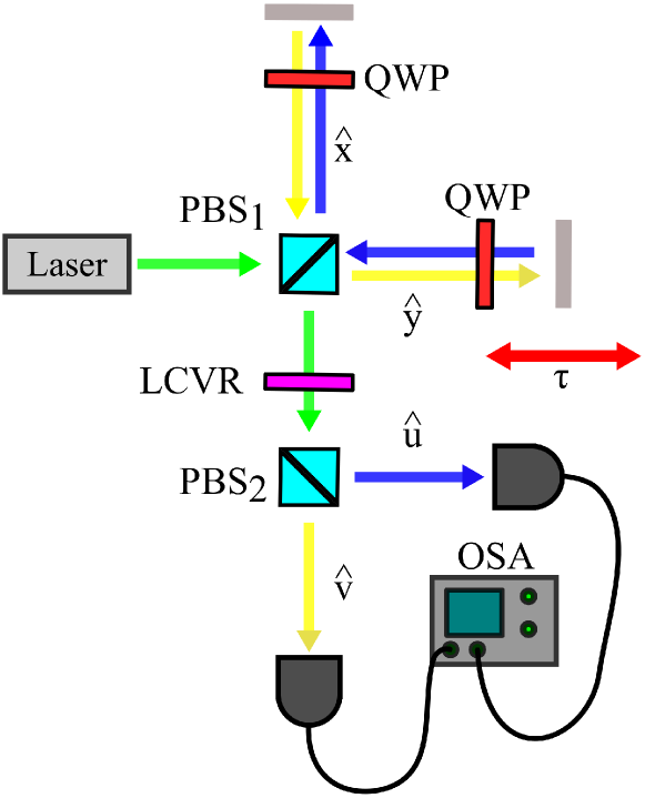
Figure 1: Weak value amplification scheme aimed at detecting extremely small temporal delays. The input pulse polarisation state is selected to be left-circular by using a polariser, a quarter-wave plate (QWP) and a half-wave plate (HWP). A first polarising beam splitter (PBS₁) splits the input into two orthogonal linear polarisations that propagate along different arms of the interferometer. An additional QWP is introduced in each arm to rotate the beam polarisation by $90^{\circ}$ to allow the recombination of both beams, delayed by a temporal delay $\tau$, in a single beam by the same PBS. After PBS₁, the output polarisation state is selected with a liquid crystal variable retarder (LCVR) followed by a second polarising beam splitter (PBS₂). The variable retarder is used to set the parameter $\theta$ experimentally. Finally, the spectrum of each output beam is measured using an optical spectrum analyzer (OSA). ($\hat{x}$,$\hat{y}$) and ($\hat{u}$,$\hat{v}$) correspond to two sets of orthogonal polarisations. Figure drawn by one of the authors (Luis-Jose Salazar Serrano).

Let us be more specific about how all these ingredients are realized in the scheme depicted in Fig. 1. An input coherent laser beam ($N$ photons) shows circular polarisation, ${\bf e}_{\mathrm{in}}=1/\sqrt{2}\,\left(\hat{x}-i\hat{y}\right)$, and a Gaussian shape with temporal width $T_{0}$ (Full-width-half maximum, $\tau\ll T_{0}$). The normalized temporal and spectral shapes of the pulse read

$$\Psi(t)=\left(\frac{4\ln 2}{\pi T_{0}^{2}}\right)^{1/4}\exp\left(-\frac{2\ln 2t^{2}}{T_{0}^{2}}\right)$$

$$\Psi(f)=\left(\frac{\pi T_{0}^{2}}{\ln 2}\right)^{1/4}\exp\left(-\frac{\pi^{2}T_{0}^{2}f^{2}}{2\ln 2}\right).$$ (1)

The input beam is divided into the two arms of a Michelson interferometer with the help of a polarising beam splitter (PBS₁). Light beams with orthogonal polarisations traversing each arm of the interferometer are delayed $\tau_{0}$ and $\tau_{0}+\tau$, respectively, which constitute the weak coupling between the two degrees of freedom. After recombination of the two orthogonal signals in the same PBS₁, the combination of a liquid-crystal variable retarder (LCVR) and a second polarising beam splitter (PBS₂) performs the post-selection of the polarisation of the output state, projecting the incoming signal into the polarisation states $\hat{u}=1/\sqrt{2}\left[\hat{x}+\hat{y}\exp(i\theta)\right]$ and $\hat{v}=1/\sqrt{2}\left[\hat{x}-\hat{y}\exp(i\theta)\right]$. The amplitudes of the signals in the two output ports write (not normalized)

$$\Phi_{u}(\tau)=\frac{\Psi(\Omega)}{2}\exp\left[i(\omega_{0}+\Omega)\tau_{0}\right]\left\{1+\exp\left[i(\omega_{0}+\Omega)\tau-i\Gamma\right]\right\}$$ (2)

$$\Phi_{v}(\tau)=\frac{\Psi(\Omega)}{2}\exp\left[i\left(\omega_{0}+\Omega\right)\tau_{0}\right]\left\{1-\exp\left[i(\omega_{0}+\Omega)\tau-i\Gamma\right]\right\},$$ (3)

where $\Gamma=\pi/2+\theta$.

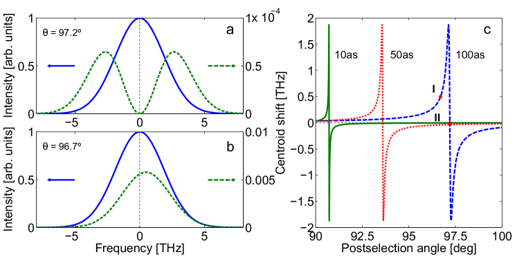
Figure 2: Spectrum measured at the output. (a) and (b): Spectral shape of the mode functions for $\tau=0$ (solid blue line) and $\tau=100$ as (dashed green line). In (a) the post-selection angle $\theta$ is $97.2^{\circ}$, so as to fulfil the condition $\omega_{0}\tau-\Gamma=\pi$. In (b) the angle $\theta$ is $96.7^{\circ}$. (c) Shift of the centroid of the spectrum of the output pulse after projection into the polarisation state $\hat{u}$ in PBS₂, as a function of the post-selection angle $\theta$. Green solid line: $\tau=10$ as; Dotted red line: $\tau=50$ as, and dashed blue line: $\tau=100$ as. Label I corresponds to $\theta=96.7^{\circ}$ [mode for $\tau=100$ as shown in (b)]. Label II corresponds to $\theta=97.2^{\circ}$, where the condition $\omega_{0}\tau-\Gamma=\pi$ is fulfiled [mode for $\tau=100$ shown in (a)]. It yields the minimum mode overlap between states with $\tau=0$ and $\tau\neq 0$. Data: $\lambda_{0}=1.5\,\mu$m and $T_{0}=100$ fs.

After the signal projection performed after PBS₂, the WVA scheme distinguishes different states, corresponding to different values of the temporal delay $\tau$, by measuring the spectrum of the outgoing signal in the selected output port. The different spectra obtained for delays $\tau=0$ and $\tau=100$ as, for two different polarisation projections, are shown in Figures 2 (a) and 2 (b). To characterize different modes one can measure, for instance, the centroid of the spectrum. Fig. 2 (c) shows the centroid shift of the output signal for $\tau\neq 0$, which reads

$$\Delta f=-\frac{\tau\,\ln 2}{\pi T_{0}^{2}}\frac{\gamma\sin\left(\omega_{0}\tau-\Gamma\right)}{1+\gamma\cos\left(\omega_{0}\tau-\Gamma\right)},$$ (4)

The differential power between both signals (with $\tau=0$ and $\tau\neq 0$) reads

$$\frac{P_{\mathrm{out}}(\tau)-P_{\mathrm{out}}(\tau=0)}{P_{\mathrm{in}}}=\frac{1}{2}\,\left[\cos\Gamma-\cos\left(\omega_{0}\tau-\Gamma\right)\right]$$ (5)

When there is no polarisation-dependent time delay ($\tau=0$), the centroid of the spectrum of the output signal is the same than the centroid of the input laser beam, i.e., there is no shift of the centroid ($\Delta f=0$). However, the presence of a small $\tau$ can produce a large and measurable shift of the centroid of the spectrum of the signal.

Results

View of weak value amplification from quantum estimation theory

Detecting the presence ($\tau\neq 0$) or absence ($\tau=0$) of a temporal delay between the two coherent orthogonally-polarised beams after recombination in PBS₁, but before traversing PBS₂, is equivalent to detecting which of the two quantum states,

$$|\Phi_{0}\rangle=|\Phi(\tau_{0})\rangle_{x}|\Phi(\tau_{0})\rangle_{y}$$ (6)

or

$$|\Phi_{1}\rangle=|\Phi(\tau_{0})\rangle_{x}|\Phi(\tau_{0}+\tau)\rangle_{y}$$ (7)

is the output quantum state which describes the coherent pulse leaving PBS₁. $(x,y)$ designates the corresponding polarisations. The spectral shape (mode function) $\Phi$ writes

$$\Phi(\tau_{0}+\tau)=\Psi(\Omega)\exp\left[i(\omega_{0}+\Omega)(\tau_{0}+\tau)\right],$$ (8)

where $\omega_{0}$ is the central frequency of the laser pulse, $\Omega=2\pi f$ is the angular frequency deviation from the the center frequency and $\Psi(\Omega)$ is the spectral shape of the input coherent laser signal.

The minimum probability of error that can be made when distinguishing between two quantum states is related to the trace distance between the states fuchs1999 . For two pure state, $\Phi_{0}$ and $\Phi_{1}$, the (minimum) probability of error is helstrom1976 ; ou1996 ; englert1996

$$P_{\mathrm{error}}=\frac{1}{2}\left(1-\sqrt{1-|\langle\Phi_{0}|\Phi_{1}\rangle|^{2}}\right).$$ (9)

For $\Phi_{0}=\Phi_{1}$, $P_{\mathrm{error}}=0.5$. On the contrary, to be successful in distinguishing two quantum states with low probability of error ($P_{\mathrm{error}}\sim 0$) requires $|\langle\Phi_{0}|\Phi_{1}\rangle|\sim 0$, i.e., the two states should be close to orthogonal.

The coherent broadband states considered here can be generally described as single-mode quantum states where the mode is the corresponding spectral shape of the light pulse. Let us consider two single-mode coherent beams

$$|\alpha\rangle=\exp\left(-\frac{|\alpha|^{2}}{2}\right)\sum_{n=0}^{\infty}\frac{\alpha^{n}\left(A^{\dagger}\right)^{n}}{n!}|0\rangle$$

$$|\beta\rangle=\exp\left(-\frac{|\beta|^{2}}{2}\right)\sum_{n=0}^{\infty}\frac{\beta^{n}\left(B^{\dagger}\right)^{n}}{n!}|0\rangle,$$ (10)

where $A$ and $B$ are the two modes

$$A^{\dagger}=\int d\Omega F(\Omega)a^{\dagger}(\Omega)$$

$$B^{\dagger}=\int d\Omega G(\Omega)a^{\dagger}(\Omega),$$ (11)

and $|\alpha|^{2}$ and $|\beta|^{2}$ are the mean number of photons in modes $A$ and $B$, respectively. The mode functions $F$ and $G$ are assumed to be normalized, i.e., $\int d\Omega|F(\Omega)|^{2}=\int d\Omega|G(\Omega)|^{2}=1$. The overlap between the quantum states, $|\langle\beta|\alpha\rangle|^{2}$, reads

$$|\langle\beta|\alpha\rangle|^{2}=\exp\left(-|\alpha|^{2}-|\beta|^{2}+\rho\alpha\beta^{*}+\rho^{*}\alpha^{*}\beta\right),$$ (12)

where we introduce the mode overlap $\rho$ that reads

$$\rho=\int d\Omega F(\Omega)\left[G(\Omega)\right]^{*}.$$ (13)

In order to obtain Eq. (12) we have made use of $\langle 0|B^{n}\left[A^{\dagger}\right]^{m}|0\rangle=n!\rho^{n}\delta_{nm}$. For $\rho=1$ (coherent beams in the same mode but with possibly different mean photon numbers) we recover the well-known formula for single-mode coherent beams glauber1963 : $|\langle\beta|\alpha\rangle|^{2}=\exp\left(-|\alpha-\beta|^{2}\right)$.

Making use of Eqs. (8), (12) and (13) we obtain

$$|\langle\Phi_{0}|\Phi_{1}\rangle|^{2}$$

$$=|\langle\Phi(\tau_{0})|\Phi(\tau_{0})\rangle_{x}|^{2}|\langle\Phi(\tau_{0})|\Phi(\tau_{0}+\tau)\rangle_{y}|^{2}$$

$$=\exp\left[-N\left(1-\gamma\cos\omega_{0}\tau\right)\right],$$ (14)

where

$$\gamma=\exp\left(-\ln 2\,\frac{\tau^{2}}{T_{0}^{2}}\right).$$ (15)

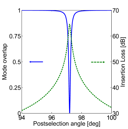
Figure 3: Mode overlap and insertion loss as a function of the post-selection angle. Mode overlap $\rho$ of the mode functions corresponding to the quantum states with $\tau=0$ and $\tau=100$ as, as a function of the post-selection angle $\theta$ (solid blue line). The insertion loss, given by $10\log_{10}\,P_{\mathrm{out}}/P_{\mathrm{in}}$ is indicated by the dotted green line. The minimum mode overlap, and maximum insertion loss, corresponds to the post-selection angle $\theta$ that fulfils the condition $\omega_{0}\tau-\Gamma=\pi$, which corresponds to $\theta=97.2^{\circ}$. Data: $\lambda_{0}=1.5\,\mu$m, $T_{0}=100$ fs.

In the WVA scheme considered here, the signal after PBS₂ is projected into the orthogonal polarisation states $\hat{u}$ and $\hat{v}$, and as a result the signals in both output ports are given by Eqs. (2) and (3). Making use of Eqs. (2), (3) and (13) one obtains that the mode overlap (for $\Phi_{u}$) reads

$$\rho=\frac{1+\cos\Gamma+\gamma\cos\omega_{0}\tau+\gamma\cos(\omega_{0}\tau-\Gamma)-i\left[\sin\Gamma+\gamma\sin\omega_{0}\tau+\gamma\sin(\omega_{0}\tau-\Gamma)\right]}{2\left[1+\cos\Gamma\right]^{1/2}\left[1+\gamma\cos(\omega_{0}\tau-\Gamma)\right]^{1/2}}.$$ (16)

For $\tau=0$, and therefore $\gamma=1$, we obtain $\rho=1$. Fig. 3 shows the mode overlap of the signal in the corresponding output port for a delay of $\tau=100$ as. The mode overlap has a minimum for $\omega_{0}\tau-\Gamma=\pi$, where the two mode functions becomes easily distinguishable, as shown in Fig. 2 (a). The effect of the polarisation projection, a key ingredient of the WVA scheme, can be understood as a change of the mode overlap (mode distinguishability) between states with different delay $\tau$.

However, an enhanced mode distinguishability in this output port is accompanied by a corresponding increase of the insertion loss, as it can be seen in Fig. 3. The insertion loss, $P_{\mathrm{out}}(\tau)/P_{\mathrm{in}}=1/2\,\left[1+\gamma\cos(\omega_{0}\tau-\Gamma)\right]$, is the largest when the modes are close to orthogonal ($\rho\sim 0$). Both effects indeed compensate, as it should be, since WVA implements unitary transformations, and the trace distance between quantum states is preserved under unitary transformations. The quantum overlap between the states reads

$$|\langle\Phi_{u}(\tau_{0})|\Phi_{u}(\tau_{0}+\tau)\rangle|^{2}=|\langle\Phi_{v}(\tau_{0})|\Phi_{v}(\tau_{0}+\tau)\rangle|^{2}$$

$$=\exp\left[-\frac{N}{2}\left(1-\gamma\cos\omega_{0}\tau\right)\right],$$ (17)

so

$$|\langle\Phi_{0}|\Phi_{1}\rangle|^{2}$$

$$=|\langle\Phi_{u}(\tau_{0})|\Phi_{u}(\tau_{0}+\tau)\rangle_{u}|^{2}|\langle\Phi_{v}(\tau_{0})|\Phi_{v}(\tau_{0}+\tau)\rangle_{v}|^{2}$$

$$=\exp\left[-N\left(1-\gamma\cos\omega_{0}\tau\right)\right],$$ (18)

which is the same result [see Eq. (14)] obtained for the signal after PBS₁, but before PBS₂.

We can also see the previous results from a slightly different perspective making use of the Cramér-Rao inequality helstrom1976 . The WVA scheme considered throughout can be thought as a way of estimating the value of the single parameter $\tau$ with the help of a light pulse in a coherent state $|\alpha\rangle$. Since the quantum state is pure, the minimum variance that can show any unbiased estimation of the parameter $\tau$, the Cramér-Rao inequality, reads

$$\mathrm{Var}\left(\hat{\tau}\right)\geq\frac{1}{4}\left[\langle\frac{\partial\alpha}{\partial\tau}|\frac{\partial\alpha}{\partial\tau}\rangle-\left|\langle\alpha|\frac{\partial\alpha}{\partial\tau}\rangle\right|^{2}\right]^{-1},$$ (19)

Making use of Eq. (7), one obtains that here the Cramér-Rao inequality reads derivative

$$\mathrm{Var}\left(\hat{\tau}\right)\geq\frac{1}{2N\left(\omega_{0}^{2}+B^{2}\right)}$$ (20)

where $B=\sqrt{2\ln 2}/T_{0}$ is the rms bandwidth in angular frequency of the pulse. In all cases of interest $B\ll\omega_{0}$. The Cramér-Rao inequality is a fundamental limit that set a bound to the minimum variance that any measurement can achieve. It is unchanged by unitary transformations and only depends on the quantum state considered.

Inspection of Eqs. (14) and (18) seems to indicate that a measurement after projection in any basis, the core element of the weak amplification scheme, provides no fundamental metrological advantage. Notice that this result implies that the only relevant factor limiting the sensitivity of detection is the quantum nature of the light used (a coherent state in our case). To obtain this result, we are implicitly assuming that a) we have full access to all relevant characteristics of the output signals; and b) detectors are ideal, and can detect any change, as small as it might be, if enough signal power is used. If this is the case, weak value amplification provides no enhancement of the sensitivity.

However, this can be far from truth in many realistic experimental situations. In the laboratory, the quantum nature of light is an important factor, but not the only one, limiting the capacity to measure tiny changes of variables of interest. On the one hand, most of the times we detect only certain characteristic of the output signals, probably the most relevant, but this is still partial information about the quantum state. On the other hand, detectors are not ideal and noteworthy limitations to its performance can appear. To name a few, they might no longer work properly above a certain photon number input, electronics and signal processing of data can limit the resolution beyond what is allowed by the specific quantum nature of light, conditions in the laboratory can change randomly effectively reducing the sensitivity achievable in the experiment. Surely, all of these are technical rather than fundamental limitations, but in many situations the ultimate limit might be technical rather than fundamental. In this scenario, we show below that weak value amplification can be a valuable and an easy option to overcome all of these technical limitations, as it has been demonstrated in numerous experiments.

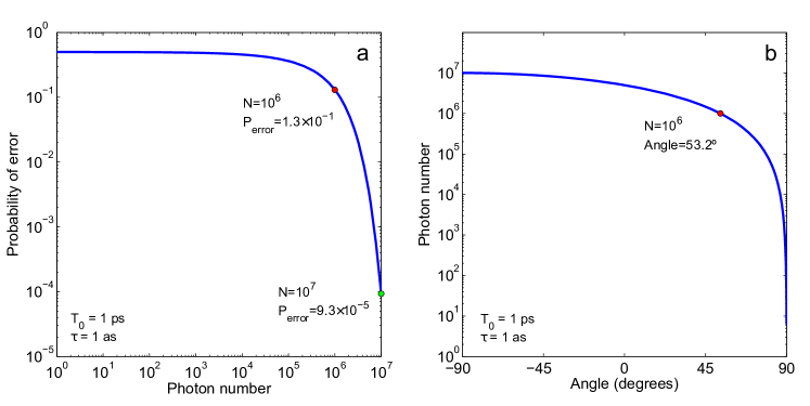
Figure 4: Reduction of the probability of error using a weak value amplification scheme. (a) Minimum probability of error as a function of the photon number $N$ that leaves the interferometer. The two points highlighted corresponds to $N=10^{6}$, which yields $P_{\mathrm{error}}=1.3\times 10^{-1}$, and $N=10^{7}$, which yields $P_{\mathrm{error}}=9.3\times 10^{-5}$. (b) Number of photons ($N_{\mathrm{out}}$) after projection in the polarisation state $\hat{u}=1/\sqrt{2}\left[\hat{x}+\hat{y}\exp(i\theta)\right]$, as a function of the angle $\theta$. The input number of photons is $N=10^{7}$. The dot corresponds to the point $N_{\mathrm{out}}=10^{6}$ and $\theta=53.2^{\circ}$. Pulse width: $T_{0}$=1 ps; temporal delay: $\tau$= 1 as.

Discussion

Advantages of using weak value amplification (I): when the detector cannot work above a certain photon number.

Let us suppose that we have at hand light detectors that cannot be used with more than $N_{0}$ photons. Any limitation on the detection time or the signal power would produce such limitation. The technical advantages of using WVA in this scenario has been previously pointed out jordan2014 . Here we make this apparent from a quantum estimation point of view, and quantify this advantage.

Fig. 4(a) shows the minimum probability of error as a function of the number of photons ($N$) entering (and leaving) the interferometer. For $N_{0}=10^{6}$, inspection of the figure shows that the probability of error is $P_{\mathrm{error}}=1.3\times 10^{-1}$. This is the best we can do with this experimental scheme and these particular detectors without resorting to weak value amplification. However, if we project the output signal from the interferometer into a specific polarisation state, and increase the flux of photons, we can decrease the probability of error, without necessarily going to a regime of high depletion of the signal torres2012 . For instance, with $\theta=53.2^{\circ}$, and a flux of photons of $N=10^{7}$, so that after projection $N_{\mathrm{out}}=10^{6}$ photons reach the detector, the probability of error is decreased to $P_{\mathrm{error}}=9.3\times 10^{-5}$, effectively enhancing the sensitivity of the experimental scheme (see Fig. 4(b)). The probability of error can be further decreased, also for other projections, at the expense of further increasing the input signal $N$.

In general, the minimum quantum overlap achievable between the states without any projection is

$$|\langle\Phi_{0}|\Phi_{1}\rangle|^{2}=\exp\left[-N_{0}\left(1-\gamma\cos\omega_{0}\tau\right)\right],$$ (21)

while making use of projection in a weak value amplification scheme is

$$|\langle\Phi_{0}|\Phi_{1}\rangle|^{2}=\exp\left[-\frac{2N_{0}\left(1-\gamma\cos\omega_{0}\tau\right)}{1+\gamma\cos\left(\omega_{0}\tau-\Gamma-\pi/2\right)}\right].$$ (22)

Eq. (22) shows that when the number of photons that the detection scheme can handle is limited ($N_{0}$), projection into a particular polarisation state, at the expense of increasing the signal level, is advantageous. From a quantum estimation point of view, WVA increases the minimum probability of error reachable, since the projection makes possible to use the maximum number of photons available ($N_{0}$) with a corresponding enhanced mode overlap. Notice that the effect of using different polarisation projections can be beautifully understood as reshaping of the balance between signal level and mode overlap.

Advantages of using weak value amplification (II): when the detector cannot differentiate between two signals

As second example, let us consider that specific experimental conditions makes hard, even impossible, to detect very similar modes, i.e., with mode overlap $\rho\sim 1$. We can represent this by assuming that there is an effective mode overlap ($\rho_{\mathrm{eff}}$) which takes into account all relevant experimental limitations of a specific set-up, given by

$$\rho\Longrightarrow\rho_{\mathrm{eff}}=1-(1-\rho)\exp\left[-\left(\frac{\rho}{a}\right)^{n}\right].$$ (23)

Fig. 5 shows an example where we assume that detected signals corresponding to $\rho>0.9$ cannot be safely distinguished due to technical restrictions of the detection system. For $\rho>0.9$, $\rho_{\mathrm{eff}}=1$, so the detection system cannot distinguish the states of interest even by increasing the level of the signal. On the contrary, for smaller values of $\rho$, accessible making use of a weak amplification scheme, this limitation does not exist since the detection system can resolve this modes when enough signal is present.

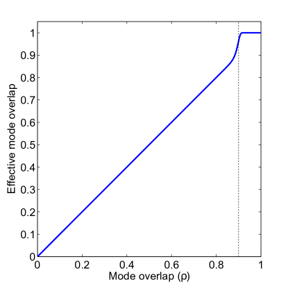
Figure 5: Effective mode overlap. For $\rho>0.9$ the detection system cannot distinguish the states of interest. Data: $a=0.9$ and $n=100$.

Advantages of using weak value amplification (III): enhancement of the Fisher information

Up to now, we have used the concept of trace distance to look for the minimum probability of error achievable in any measurement when using a given quantum state. In doing that, we only considered how the quantum state changes for different values of the variable to be measured, without any consideration of how this quantum state is going to be detected. If we would like to include in the analysis additional characteristics of the detection scheme, one can use the concept of Fisher information, that requires to consider the probability distribution of possible experimental outcomes for a given value of the variable of interest. In this approach, one chooses different probability distributions to describe formally characteristics of specific detection scheme jordan2014 .

Let us assume that to estimate the value of the delay $\tau$, we measure the shift of the centroid ($\Delta f$) of the spectrum $\Phi_{u}(\tau)$, given by Eq. (3). A particular detection scheme will obtain a set of results $\left\{(\Delta f)_{i}\right\}$, $i=1..N$ for a given delay $\tau$. $N$ is the number of photons detected. The Fisher information $I(\tau)$ provides a bound of $\mathrm{Var}\left(\hat{\tau}\right)$ for any unbiased estimator when the probability distribution $p(\left\{(\Delta f)_{i}\right\}|\tau)$ of obtaining the set $\left\{(\Delta f)_{i}\right\}$, for a given $\tau$, is known. If we assume that the probability distribution $p(\left\{(\Delta f)_{i}\right\}|\tau)$ is Gaussian, with mean value $\Delta f$ given by Eq. (4) and variance $\sigma^{2}$, determined by the errors inherent to the detection process, the Fisher information reads fisher1

$$I(\tau)=\frac{N}{\sigma^{2}}\left[\frac{\partial\Delta f}{\partial\tau}\right]^{2}$$ (24)

where

$$\frac{\partial\Delta f}{\partial\tau}=\frac{\gamma B^{2}\left[B^{2}\tau^{2}\sin\phi-\omega_{0}\tau\left(\gamma+\cos\phi\right)-\sin\phi\left(1+\gamma\cos\phi\right)\right]}{2\pi\,\left(1+\gamma\cos\phi\right)^{2}}$$ (25)

and $\phi=\omega_{0}\tau-\Gamma$.

For $\phi=0$, i.e., the angle of post-selection is $\theta=-\pi/2+\omega_{0}\tau$, the Fisher information is

$$I_{0}=\frac{N_{0}}{2}\left(1+\gamma\right)\times\frac{\gamma^{2}B^{4}(\omega_{0}\tau)^{2}}{2\pi\sigma^{2}(1+\gamma)^{2}}=\frac{\gamma^{2}B^{4}(\omega_{0}\tau)^{2}}{4\pi\sigma^{2}(1+\gamma)}$$ (26)

Notice that $\theta=-\pi/2$ corresponds to considering equal input and output polarization state, i.e., no weak value amplification scheme. For $\phi=\pi$, where the angle of post-selection is $\theta=\pi/2+\omega_{0}\tau$, we have

$$I_{\pi}=\frac{N_{0}}{2}\left(1-\gamma\right)\times\frac{\gamma^{2}B^{4}(\omega_{0}\tau)^{2}}{2\pi\sigma^{2}(1-\gamma)^{2}}=\frac{\gamma^{2}B^{4}(\omega_{0}\tau)^{2}}{4\pi\sigma^{2}(1-\gamma)}$$ (27)

$\theta=\pi/2$ corresponds to considering an output polarisation state orthogonal to the input polarisation state i.e., when the effect of weak value amplification is most dramatic, as it can be easily observed in Fig. 2(a). The Fisher bound for $\Phi=\pi$ is a factor $I_{\pi}/I_{0}=(1+\gamma)/(1-\gamma)$ larger than the bound for $\Phi=0$, so WVA achieves enhancement of the Fisher information. This Fisher information enhancement effect, which does not happen always, it has been observed for certain WVA schemes viza2013 ; jordan2014 .

There is no contradiction between the facts that the minimum probability of error, obtained by making use of the concept of trace distance, is not changed by WVA, while at the same time there can be enhancement of the Fisher information. By selecting a particular probability distribution to evaluate the Fisher information, we include information about the detection scheme. In our case, we estimate the value of $\tau$ by measuring the $\tau$-dependent shift of the centroid of the spectrum of the signal in one output port after PBS₂, which is only part of all the information available, given by the full signal in Eqs. (2) and (3). We also assumed a Gaussian probability distribution with a constant variance $\sigma^{2}$ independent of $\tau$. The Cramér-Rao bound we have derived here depends on the full information available (the quantum state) before any particular detection. An unitary transformation, as WVA is, does not modify the bound. On the contrary, the Fisher information, by using a particular probability distribution to describe the possible outcomes in an particular experiment, selects certain aspects of the quantum state to be measured (partial information), and this bound can change in a WVA scheme, although the bound should be always above the Cramér-Rao bound. In this restrictive scenario, the use of certain polarization projections can be preferable.

The existence and nature of these different bounds might possibly explain certain confusion about the capabilities of WVA, whether WVA is considered to provide any metrological advantage or not. On the one hand, if we consider the trace distance, or the quantum Cramér-Rao inequality, without any consideration about how the quantum states are detected, post-selection inherent in WVA does not lower the minimum probability of error achievable, so from this point of view WVA offers no metrological advantage. On the other hand, in certain scenarios, the Fisher information, when it takes into account information about the detection scheme, can be enhanced due to post-selection. In this sense, one can think of WVA as an advantageous way to optimize a particular detection scheme.

Conclusions

WVA schemes makes use of linear optics unitary transformations. Therefore, if the only limitations in a measurement are due to the quantum nature (intrinsic statistics) of the light, for instance, the presence of Shot noise in the case of coherent beams, WVA does not offer any advantage regarding any decrease of the minimum probability of error achievable. This is shown by making use of the trace distance between quantum states or the Cramér-Rao inequality, which set sensitivity bounds that are independent of any particular post-selection. However, notice that this implicitly assume that full information about the quantum states used can be made available, and detectors are ideal, so they can detect any change of the variable of interest, as small as it might be, provided there is enough signal power.

Nevertheless, these assumptions are in many situations of interest far from true. These limitations, sometimes refereed as technical noise, even though not fundamental (one can always imagine using a better detector or a different detection scheme) are nonetheless important, since they limit the accuracy of specific detection systems at hand. In these scenarios, the importance of weak value amplification is that by decreasing the mode overlap associated with the states to be measured and possibly increasing the intensity of the signal, the weak value amplification scheme allows, in principle, to distinguish them with lower probability of error.

We have explored some of these scenarios from an quantum estimation theory point of view. For instance, we have seen that when the number of photons usable in the measurement is limited, the minimum probability of error achievable can be effectively decreased with weak value amplification. We have also analyzed how weak value amplification can differentiate between in practice-indistinguishable states by decreasing the mode overlap between its corresponding mode functions.

Finally we have discussed how the confusion about the usefulness of weak value amplification can possibly derive from considering different bounds related to how much sensitivity can, in principle, be achieved when estimating a certain variable of interest. One might possibly say that the advantages of WVA have nothing to do with fundamental limits and should not be viewed as addressing fundamental questions of quantum mechanics caves2014 . However, from a practical rather than fundamental point of view, the use of WVA can be advantageous in experiments where sensitivity is limited by experimental (technical), rather than fundamental, uncertainties. In any case, if a certain measurement is optimum depends on its capability to effectively reach any bound that might exist.

References

Figure Captions

Figure1

Weak value amplification scheme aimed at detecting extremely small temporal delays. The input pulse polarisation state is selected to be left-circular by using a polariser, a quarter-wave plate (QWP) and a half-wave plate (HWP). A first polarising beam splitter (PBS₁) splits the input into two orthogonal linear polarisations that propagate along different arms of the interferometer. An additional QWP is introduced in each arm to rotate the beam polarisation by $90^{\circ}$ to allow the recombination of both beams, delayed by a temporal delay $\tau$, in a single beam by the same PBS. After PBS₁, the output polarisation state is selected with a liquid crystal variable retarder (LCVR) followed by a second polarising beam splitter (PBS₂). The variable retarder is used to set the parameter $\theta$ experimentally. Finally, the spectrum of each output beam is measured using an optical spectrum analyzer (OSA). ($\hat{x}$,$\hat{y}$) and ($\hat{u}$,$\hat{v}$) correspond to two sets of orthogonal polarisations.

Figure2

Spectrum measured at the output. (a) and (b): Spectral shape of the mode functions for $\tau=0$ (solid blue line) and $\tau=100$ as (dashed green line). In (a) the post-selection angle $\theta$ is $97.2^{\circ}$, so as to fulfil the condition $\omega_{0}\tau-\Gamma=\pi$. In (b) the angle $\theta$ is $96.7^{\circ}$. (c) Shift of the centroid of the spectrum of the output pulse after projection into the polarisation state $\hat{u}$ in PBS₂, as a function of the post-selection angle $\theta$. Green solid line: $\tau=10$ as; Dotted red line: $\tau=50$ as, and dashed blue line: $\tau=100$ as. Label I corresponds to $\theta=96.7^{\circ}$ [mode for $\tau=100$ as shown in (b)]. Label II corresponds to $\theta=97.2^{\circ}$, where the condition $\omega_{0}\tau-\Gamma=\pi$ is fulfiled [mode for $\tau=100$ shown in (a)]. It yields the minimum mode overlap between states with $\tau=0$ and $\tau\neq 0$. Data: $\lambda_{0}=1.5\,\mu$m and $T_{0}=100$ fs.

Figure3

Mode overlap and insertion loss as a function of the post-selection angle. Mode overlap $\rho$ of the mode functions corresponding to the quantum states with $\tau=0$ and $\tau=100$ as, as a function of the post-selection angle $\theta$ (solid blue line). The insertion loss, given by $10\log_{10}\,P_{\mathrm{out}}/P_{\mathrm{in}}$ is indicated by the dotted green line. The minimum mode overlap, and maximum insertion loss, corresponds to the post-selection angle $\theta$ that fulfils the condition $\omega_{0}\tau-\Gamma=\pi$, which corresponds to $\theta=97.2^{\circ}$. Data: $\lambda_{0}=1.5\,\mu$m, $T_{0}=100$ fs.

Figure4

Reduction of the probability of error using a weak value amplification scheme. (a) Minimum probability of error as a function of the photon number $N$ that leaves the interferometer. The two points highlighted corresponds to $N=10^{6}$, which yields $P_{\mathrm{error}}=1.3\times 10^{-1}$, and $N=10^{7}$, which yields $P_{\mathrm{error}}=9.3\times 10^{-5}$. (b) Number of photons ($N_{\mathrm{out}}$) after projection in the polarisation state $\hat{u}=1/\sqrt{2}\left[\hat{x}+\hat{y}\exp(i\theta)\right]$, as a function of the angle $\theta$. The input number of photons is $N=10^{7}$. The dot corresponds to the point $N_{\mathrm{out}}=10^{6}$ and $\theta=53.2^{\circ}$. Pulse width: $T_{0}$=1 ps; temporal delay: $\tau$= 1 as.

Figure5

Effective mode overlap. For $\rho>0.9$ the detection system cannot distinguish the states of interest. Data: $a=0.9$ and $n=100$.

Acknowledgements We acknowledge support from the Severo Ochoa program (Government of Spain), from the ICREA Academia program (ICREA, Generalitat de Catalunya) and from Fundació Privada Cellex, Barcelona.

Author Contributions All authors contribute equally to the paper and reviewed the manuscript.

Additional information Competing financial interests: The authors declare no competing financial interests.

References

- (1) Aharonov, Y., Albert, D. Z. & Vaidman, L. How the result of a measurement of a component of the spin of a spin-1/2 particle can turn out to be 100. Phys. Rev. Lett. 60, 1351–1354 (1988).
- (2) Hosten, O. & Kwiat, P. Observation of the spin Hall effect of light via weak measurements, Science 319, 787–790 (2008).
- (3) Zhou, X., Zhou, Ling, X., Luo H., & Wen, S. Identifying graphene layers via spin Hall effect of light. App. Phys. Lett. 101, 251602 (2012).
- (4) Ben Dixon P., Starling, D. J., Jordan, A. N., & Howell, J. C. Ultrasensitive beam deflection measurement via interferometric weak value amplification. Phys. Rev. Lett. 102, 173601 (2009).
- (5) Pfeifer, M., & Fischer, P. Weak value amplified optical activity measurements. Opt. Express 19, 16508–16517 (2011).
- (6) Howell, J. C., Starling, D. J., Dixon, P. B., Vudyasetu, K. P. & Jordan, A. N. Precision frequency measurements with interferometric weak values. Phys. Rev. A 82, 063822 (2010).
- (7) Egan, P. & Stone, J. A. Weak-value thermostat with 0.2 mK precision. Opt. Lett. 37, 4991–4993 (2012).
- (8) Xu, X. Y. et al. Phase estimation with weak measurement using a white light source. Phys. Rev. Lett. 111, 033604 (2013).
- (9) Dressel, J., Malik, M., Miatto, F. M., Jordan, A. N. & Boyd R. W. Colloquium: Understanding quantum weak values: Basics and applications. Rev. Mod. Phys. 86, 307–316 (2014).
- (10) Jordan, A. N., Martíez-Rincón, J. & Howell, J. C. Technical Advantages for Weak-Value Amplification: When Less Is More. Phys. Rev. X 4, 011031 (2014).
- (11) Knee, G. C., & Gauger, E. M. When Amplification with Weak Values Fails to Suppress Technical Noise. Phys. Rev. X 4, 011032 (2014).
- (12) Ferrie, C. & Combes, J. Weak Value Amplification is Suboptimal for Estimation and Detection. Phys. Rev. Lett. 112, 040406 (2014).
- (13) Vaidman, L. Comment on Weak value amplification is sub-optimal for estimation and detection. Phys. Rev. Lett. 111, 033604 (2013). arXiv:1402.0199v1 [quant-ph] (2014).
- (14) Helstrom, C. W. Quantum Detection and Estimation Theory, Academic press Inc. 1976.
- (15) Nielse, M. A. & Chuang I. L. Quantum computation and quantum information, Cambridge University Press, 2000.
- (16) Zhang, L., Datta, A. & Walsmely, I. A. Precision metrology using weak measurements. Phys. Rev. Lett. 114, 210801 (2015)
- (17) Torres, J. P., Puentes, G., Hermosa, N. & Salazar-Serrano, L. J. Weak interference in the high-signal regime. Opt. Express 20, 18869-18875 (2012).
- (18) Duck, I. M., Stevenson, P. M. & Sudarhshan, E. C. G. The sense in which a weak measurement of a spin-1/2 particles’s spin component yields a value of 100. Phys. Rev. D 40, 2112–2117 (1989).
- (19) Howell, J. C., Starling, D. J., Dixon, P. B., Vudyasetu, K. P. & Jordan, A. N. Interferometric weak value deflections: quantum and classical treatments. Phys. Rev. A 81, 033813 (2010).
- (20) Ritchie, N. W., Story, J. G. & Hulet, R. G. Realization of a measuremernt of a weak value. Phys. Rev. Lett. 66 1107–1110 (1991).
- (21) Brunner, N. & Simon, C. Measuring small longitudinal phase shifts: weak measurements of standard interferometry. Phys. Rev. Lett. 105 010405 (2010).
- (22) Salazar-Serrano, L. J., Janner, D., Brunner, N., Pruneri, V. & Torres, J. P. Measurement of sub-pulse-width temporal delays via spectral interference induced by weak value amplification. Phys. Rev. A 89 012126 (2014).
- (23) Strubi, G. & Bruder, C. Measuring Ultrasmall Time Delays of Light by Joint Weak Measurements. Phys. Rev. Lett. 110 083605 (2012).
- (24) Li, C.-F. et al. Ultrasensitive phase estimation with white light. Phys. Rev. A 83, 044102 (2011).
- (25) Fuchs, C. A., & van de Graaf, J. Cryptographic Distinguishability Measures for Quantum Mechanical States. IEEE T. Inform. Theory 45, 1216–1227 (1999).
- (26) Englert, B.-G. Fringe Visibility and Which-Way Information: An Inequality,” Phys. Rev. Lett. 77, 2154–2157 (1996).
- (27) Ou, Z. Y. Complementarity and Fundamental Limit in Precision Phase Measurement. Phys. Rev. Lett. 77, 2352–2355 (1996).
- (28) Glauber, R. J. Coherent and incoherent states of the radiation field. Phys. Rev. 131, 2766–2788 (1966).
- (29) Let us define . For a coherent product state of the form , where the index refers to different frequency modes, one obtains that , where . If , where is the mean number of photons in frequency mode and only depends on the parameter as , one obtains that , where is the creation operator of the corresponding frequency mode.
- (30) The unknown parameter of interest has value . After repeated measurements to estimate its value, we obtain a distribution of outcomes which can be characterized by a probability distribution that depends on the value of . The Fisher information reads . The variance of any unbiased estimator that makes use of the ensemble is bounded from below by . When the Fisher function can be written as , where is the variable that we measure, the Fisher information can be written as .
- (31) Viza, G. I. et al. Weak-values technique for velocity measurements. Opt. Lett. 38, 2949-2952 (2013).
- (32) Combes, J. & Ferrie, C. & Zhang, J., and Carlton M. Caves, C. M. Quantum limits on postselected, probabilistic quantum metrology, Phys. Rev. A 89, 052117 (2014).