Rank-1 accelerated illumination recovery in scanning diffractive imaging by transparency estimation.

Abstract

We consider the problem of blind ptychography, that is the joint estimation of an unknown object and an illumination function from diffraction intensity measurements. In ptychography, diffraction measurements from neighboring regions of the same object are related to each other by a pairwise relationship between overlapping frames. When the illumination is well known, the relationship among frames is given by a linear projection operator. We propose a power iteration-projection algorithm that minimizes the global pairwise discrepancy among frames. We accelerate the convergence of power method by subtracting the estimated localized average transparency of the unknown object. The method is effective for weakly scattering and low contrast objects or piecewise smooth specimens.

Ptychography is an increasingly popular technique to achieve diffraction limited imaging over a large field of view without the need for high quality optics Hoppe:1969 ; Hegerl_Hoppe:1970 ; batesptycho ; spence:book ; Chapman1996 ; Thibault2008 ; Thibault2009 ; pie2 ; Kewish2010 ; Honig:11 ; guizar-mirror ; Maiden:2012 ; axel ; Thibault-Guizar ; Godard:12 ; clark:2011 ; fourierptycho ; batey2014information ; dong2014spectral ; marrison2013ptychography ; tian2014multiplexed ; vine2009ptychographic ; stockmar2013near . Since the reconstruction of ptychographic data is a non-linear problem, there are still many open problemssynchroAP , nevertheless the phase retrieval problem is made tractable by recording multiple diffraction patterns from the same region of the object, compensating phase-less information with a redundant set of measurements. Data redundancy enables to handle experimental uncertainties as well. Methods to work with unknown illuminations or “lens” were proposedChapman1996 ; Thibault2008 ; Thibault2009 ; pie2 ; hesse2015proximal . They are now used to calibrate high quality x-ray optics Kewish2010 ; Honig:11 ; guizar-mirror , EUV lithography toolswojdyla:2014 , x-ray lasers ptychoxfel and space telescopes spacetelescopes . More recently, position errorsfienup ; Maiden:2012 ; axel , backgroundthurman2009 ; guizar:bias , noise statistics Thibault-Guizar ; Godard:12 and partially coherent illuminationclark:2011 ; Fienup:93 ; Abbey2008 ; CDIpartialcoherence . Situations when sample, illumination function, incoherent multiplexing effects, as well as positions, vibrations, binning, multiplexing, fluctuating background are unknown parameters in high dimensions have been added to the nonlinear optimization to fit the data using projections, gradient, conjugate gradient, Newton chao , and spectral methods marchesini2013augmented ; synchroAP ; batey2014information . Here we focus on the illumination retrieval problem. We utilize the notation described in marchesini2013augmented ; synchroAP , which is summarized below.

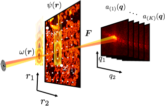
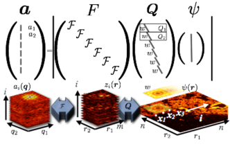
Figure 1: The measured amplitudes $\bm{\mathsf{a}}$ and the relationship with an an unknown object $\psi$ in standard “Far Field” ptychography. Geometric representation of the operators involved in simulating a ptychographic imaging experiment synchroAP ; marchesini2013augmented .

I Background

The relationship between an unknown discretized object $\psi$ , and the diffraction measurements $\bm{\mathsf{a}}_{(i)}$ collected in a ptychography experiment (see figure 1) can be represented compactly as:

$$\bm{\mathsf{a}}=|\bm{\mathsf{FQ}}\psi^{\vee}|\text{, or }\begin{cases}\bm{\mathsf{a}}=|\bm{\mathsf{F}}\bm{z}|,\\ \bm{z}=\bm{\mathsf{Q}}\psi^{\vee},\end{cases}$$ (1)

where $\psi^{\vee}$ is the object $\psi$ in vector form. Eq. (1) can be expressed as:

$$\overbracket{\left[\begin{array}[]{c}\bm{\mathsf{a}}_{(1)}\\ \vdots\\ \bm{\mathsf{a}}_{(K)}\end{array}\right]}^{\bm{\mathsf{a}}\in\mathbb{R}^{Km^{2}}}=\left|\overbracket{\left[\begin{array}[]{ccc}F&\ldots&0\\ \vdots&\ddots&\vdots\\ 0&\ldots&F\end{array}\right]}^{\bm{\mathsf{F}}\in\mathbb{C}^{Km^{2}\times Km^{2}}}\overbracket{\left[\begin{array}[]{c}\bm{z}_{(1)}\\ \vdots\\ \bm{z}_{(K)}\end{array}\right]}^{\bm{z}\in\mathbb{C}^{Km^{2}}}\right|,\quad\overbracket{\left[\begin{array}[]{c}\bm{z}_{(1)}\\ \vdots\\ \bm{z}_{(K)}\end{array}\right]}^{\bm{z}\in\mathbb{C}^{Km^{2}}}=\overbracket{\left[\begin{array}[]{c}\text{diag}(w)\bm{\mathsf{T}}_{(1)}\\ \vdots\\ \text{diag}(w)\bm{\mathsf{T}}_{(K)}\end{array}\right]}^{\bm{\mathsf{Q}}\in\mathbb{C}^{Km^{2}\times n^{2}},}\overbracket{\left[\begin{array}[]{c}\psi_{1}\\ \vdots\\ \psi_{n^{2}}\end{array}\right]}^{\psi\in\mathbb{C}^{n^{2}}}$$

where $\bm{z}$ are $K$ frames extracted from the object $\psi$ and multiplied by the illumination function $w$, $\bm{\mathsf{F}}$ is the associated 2D DFT matrix when we write everything in the stacked form, that is, $F$ is a $m^{2}\times m^{2}$ matrix satisfying $F_{lk}=\bm{e}_{l}^{T}F\bm{e}_{k}=e^{i\mathsf{q}_{m}^{-1}(l-1)\cdot\mathsf{r}_{m}^{-1}(k-1)}$. For experimental geometries related to what has been described above, such as Near Field, “Fresnel”, Fourier ptychography, through-focus dong2014spectral ; vine2009ptychographic ; stockmar2013near ; tian2014multiplexed one can substitute the simple Fourier transform with the appropriate propagator.

The illumination matrix $\bm{\mathsf{Q}}$ encodes information about illumination $w\in\mathbb{C}^{m^{2}}$, and the $K$ relative translations between the probe $w$ and the object $\psi$. In particular, the $(i)$ block denoted as $\bm{\mathsf{Q}}_{(i)}\in\mathbb{C}^{m^{2}\times n^{2}}$ extracts one frame from the object and multiplies by the illumination $w$:

$$\bm{\mathsf{Q}}_{(i)}= \overbracket{{\text{diag}}(w^{\vee})}^{\boxed{\bcancel{\quad}}}\overbracket{\bm{\mathsf{T}}_{(i)}\in\mathbb{C}^{m^{2}\times n^{2}}}^{\boxed{\quad\bcancel{\quad}\quad\quad}},\quad\bm{\mathsf{Q}}=\left(\begin{array}[]{c}{\text{diag}}(w^{\vee})\bm{\mathsf{T}}_{(1)}\\ {\text{diag}}(w^{\vee})\bm{\mathsf{T}}_{(2)}\\ \vdots\\ {\text{diag}}(w^{\vee})\bm{\mathsf{T}}_{(K)}\end{array}\right)\quad$$ (6)

where the matrix $\bm{\mathsf{T}}_{(i)}$ extract an $m\times m$ frame out of an $n\times n$ image. The matrix $T_{(i)}$ can be expressed in terms of a translation matrix $\bm{C}_{\bm{x}}$ which circularly translates by $\bm{x}$ in $D^{n\times n}$ and the restriction matrix $\bm{\mathsf{R}}$, which is of size $m^{2}\times n^{2}$ so that $\bm{\mathsf{R}}(i,i)=1$ for all $i=1,\ldots,m^{2}$ and $0$ otherwise:

$$\bm{\mathsf{T}}_{(i)}= \bm{\mathsf{R}}\bm{C}_{\bm{x}_{(i)}},\quad\bm{\mathsf{T}}=\left(\begin{array}[]{c}\bm{\mathsf{T}}_{(1)}\\ \bm{\mathsf{T}}_{(2)}\\ \vdots\\ \bm{\mathsf{T}}_{(K)}\end{array}\right)$$ (11)

In the following, to simplify the notation, we will not distinguish between $w$ (resp. $\psi$) and its vector form $w^{\vee}$ (resp. $\psi^{\vee}$) and use the same notation $w$ (resp. $\psi$). We simplify Eq (6) as

$$\bm{\mathsf{Q}}=\text{diag}(\bm{\mathsf{S}}w)\bm{\mathsf{T}}.$$ (12)

Where we define $\bm{\mathsf{S}}\in\mathbb{R}^{Km^{2}\times m^{2}}$ to be the matrix that replicates the illumination probe $w$ into $k$ stack of frames, that is, $\bm{\mathsf{S}}$ is a $K\times 1$ block matrix with the $m^{2}\times m^{2}$ identity matrix as the block. There is a relationship between $\psi$,$w$ and $\bm{z}$:

$$\bm{z}=\bm{\mathsf{Q}}\psi=\text{diag}(\bm{\mathsf{S}}w)\bm{\mathsf{T}}\psi=\text{diag}(\bm{\mathsf{T}}\psi)\bm{\mathsf{S}}w$$ (13)

due to the fact that $\text{diag}(\bm{\mathsf{S}}w)\bm{\mathsf{T}}\psi$ is the entry-wise product of $\bm{\mathsf{S}}w$ and $\bm{\mathsf{T}}\psi$.

In the notation used in this paper, projection operators are expressed as:

$$P_{\bm{\mathsf{Q}}}=\bm{\mathsf{Q}}(\bm{\mathsf{Q}}^{*}\bm{\mathsf{Q}})^{-1}\bm{\mathsf{Q}}^{*}$$

$$P_{\bm{\mathsf{a}}}=\bm{\mathsf{F}}^{*}\frac{\bm{\mathsf{F}}\bm{z}}{|\bm{\mathsf{F}}\bm{z}|}\bm{\mathsf{a}}$$

II Alternating projections probe, frames, image

The standard updateThibault2009 ; pie2 proceeds in three steps updating the estimate of the illumination $w$, estimate of the specimen $\psi$, and the frames $\bm{z}$ based on experimental geometry and data. First update the image $\psi$ by (13):

$$\psi\leftarrow (\bm{\mathsf{Q}}^{\ast}\bm{\mathsf{Q}})^{-1}\bm{\mathsf{Q}}^{\ast}\bm{z}=\frac{\bm{\mathsf{T}}^{\ast}\text{diag}(\bm{\mathsf{S}}\bar{w})\bm{z}}{\bm{\mathsf{T}}^{\ast}(\bm{\mathsf{S}}|w|^{2})},$$ (14)

where the second equality holds due to (12); that is, $\bm{\mathsf{Q}}^{\ast}\bm{\mathsf{Q}}=\text{diag}(\bm{\mathsf{T}}^{\ast}(\bm{\mathsf{S}}|w|^{2}))$. Note that for the sake of simplifying notation, we represent $\text{diag}(v)^{-1}B=:\frac{B}{v}$ when $\text{diag}(v)$ is invertible diagonal matrix. Second, by (13), update the probe $w$:

$$w\leftarrow \frac{\bm{\mathsf{S}}^{\ast}\text{diag}(\bm{\mathsf{T}}\bar{\psi})\bm{z}}{\bm{\mathsf{S}}^{\ast}\bm{\mathsf{T}}|\psi|^{2}},$$ (15)

Third update the frames using the new probe embedded in $\bm{\mathsf{Q}}$, and the $P_{\bm{\mathsf{a}}}$ operator:

$$\bm{z}\leftarrow P_{\bm{\mathsf{a}}}\text{diag}(\bm{\mathsf{S}}w)\bm{\mathsf{T}}\psi$$ (16)

Note that Equation (15) is motivated by (13). In fact, we have ${\text{diag}(\bm{\mathsf{T}}\bar{\psi})\bm{z}=\text{diag}(|\bm{\mathsf{T}}\psi|^{2})}\bm{\mathsf{S}}w$. And note that by a direct calculation, $\bm{\mathsf{S}}^{*}\text{diag}(|\bm{\mathsf{T}}\psi|^{2})\bm{\mathsf{S}}=\text{diag}(\sum_{i}\bm{\mathsf{T}}_{(i)}|\psi|^{2})$, which leads to (15) when all entries of $\bm{\mathsf{S}}^{\ast}\bm{\mathsf{T}}|\psi|^{2}$ are not zero. When there is zero entry in $\bm{\mathsf{S}}^{\ast}|\bm{\mathsf{T}}\psi|^{2}$, we may consider $\max\{\bm{\mathsf{S}}^{\ast}|\bm{\mathsf{T}}\psi|^{2},\epsilon\}$, where $\epsilon>0$ is a small positive number determined by the user. Note that $\bm{\mathsf{S}}^{*}$ plays the role of averaging.

III The relationship between probes (illumination ) and frames

We now analyze here the symmetry between $\bm{\mathsf{Q}}$ and $\bm{z}$, that is, we look at the frame-wise relationship. We note that $T_{(i)}^{\ast}Q_{(i)}=T_{(i)}^{\ast}\text{diag}(w)T_{(i)},\,\forall(i)$ is a diagonal matrix. Hence we can write the following relationship between two frames:

$$T_{(i)}^{\ast}Q_{(i)}T_{(j)}^{\ast}z_{(j)}=T_{(i)}^{\ast}Q_{(i)}T_{(j)}^{\ast}Q_{(j)}\psi =T_{(j)}^{\ast}Q_{(j)}T_{(i)}^{\ast}Q_{(i)}\psi=T_{(j)}^{\ast}Q_{(j)}T_{(i)}^{\ast}z_{(i)}$$

i.e. the i-th frame multiplied by the j-th illumination is equal to the j-th frame multiplied by the i-th illumination, after putting the results back to the right position. In other words, we have a pairwise relationship

$$\sum_{i,j}\|T_{(j)}^{\ast}Q_{(j)}T_{(i)}^{\ast}z_{(i)}-T_{(i)}^{\ast}Q_{(i)}T_{(j)}^{\ast}z_{(j)}\|=0.$$ (17)

By swapping diagonal matrices $T_{(i)}^{\ast}Q_{(i)}$ and using $T_{(i)}T_{(i)}^{\ast}=I$, we can write out the pairwise discrepancy between all frames:

$$\frac{1}{2}\sum_{i,j}\|T_{(j)}^{\ast}Q_{(j)}T_{(i)}^{\ast}z_{(i)}-T_{(i)}^{\ast}Q_{(i)}T_{(j)}^{\ast}z_{(j)}\|^{2}= \sum_{i,j}z^{\ast}_{(i)}\left[\mathbb{Q}_{(i)}^{2}\delta_{i,j}-Q_{(i)}Q_{(j)}^{\ast}\right]z_{(j)}=\bm{z}^{\ast}[\mathbb{Q}^{2}-\mathbb{P}]\bm{z}$$

where ${\mathbb{Q}}^{2}_{(i)}\equiv T_{(i)}\bm{\mathsf{Q}}^{\ast}\bm{\mathsf{Q}}T_{(i)}^{\ast}$, ${\mathbb{Q}}^{2}\equiv\text{diag}({\mathbb{Q}}^{2}_{(i=1\dots k)})$, $\mathbb{P}\equiv\bm{\mathsf{Q}}\bm{\mathsf{Q}}^{\ast}$. Indeed, note that $\sum_{ij}z_{(i)}^{*}\bm{\mathsf{T}}_{(i)}\bm{\mathsf{Q}}_{(j)}^{*}\bm{\mathsf{Q}}_{(j)}\bm{\mathsf{T}}_{(i)}^{*}z_{(i)}=\sum_{i}z_{(i)}^{*}\bm{\mathsf{T}}_{(i)}\big{[}\sum_{j}\bm{\mathsf{Q}}_{(j)}^{*}\bm{\mathsf{Q}}_{(j)}\big{]}\bm{\mathsf{T}}_{(i)}^{*}z_{(i)}$ and $\bm{\mathsf{Q}}^{*}\bm{\mathsf{Q}}=\sum_{j}\bm{\mathsf{Q}}_{(j)}^{*}\bm{\mathsf{Q}}_{(j)}$. Note that $\bm{\mathsf{Q}}^{*}\bm{\mathsf{Q}}$ is a diagonal matrix with non-negative diagonal entries describing how a pixel of the object of interest is illuminated by different windows. Thus we can define $\mathbb{Q}$ by taking square root of $\mathbb{Q}^{2}$ entry-wisely. We may assume that the diagonal is positive, otherwise some information of the object is missed in the experiment. Thus we may define $\mathbb{Q}^{-1}$. Also note that by a direct calculation, we obtain

$$\mathbb{Q}^{2}=\text{diag}(\bm{\mathsf{T}}\bm{\mathsf{T}}^{*}\bm{\mathsf{S}}|w|^{2}).$$ (18)

Intuitively, $\bm{\mathsf{T}}^{*}\bm{\mathsf{S}}|w|^{2}$ describes how pixels of the whole $\psi$ is illuminated, and $\bm{\mathsf{T}}_{(i)}\bm{\mathsf{T}}^{*}\bm{\mathsf{S}}|w|^{2}$ is how the pixels of the $i$-th patch of $\psi$ is illuminated, which is the same as $T_{(i)}\bm{\mathsf{Q}}^{\ast}\bm{\mathsf{Q}}T_{(i)}^{\ast}$.

We can minimize this functional by first renormalizing, making a change of variable $\hat{\bm{z}}=\mathbb{Q}\bm{z}$, then applying the power iteration:

$$\bm{z}^{\ast}[\mathbb{Q}^{2}-\mathbb{P}]\bm{z}=\hat{\bm{z}}^{\ast}[I-\mathbb{Q}^{-1}\mathbb{P}\mathbb{Q}^{-1}]\hat{\bm{z}}=\hat{\bm{z}}^{\ast}[I-P_{Q}]\hat{\bm{z}}$$ (19)

$$\bm{z}\leftarrow\mathbb{Q}^{-1}P_{Q}{\hat{\bm{z}}}=\mathbb{Q}^{-1}P_{Q}\mathbb{Q}{\bm{z}}=P_{Q}{\bm{z}}$$ (20)

which holds by the way $\mathbb{Q}$ is defined. The reason for the above formulation is to establish a relationship between $Q$ and $z$. As we have seen in Sec. II, the relationship between $w$ and $\psi$ in (Eq. (15)) is used to recover both $w$ and $\psi$.

Interestingly, the relationship (Eq. 17) is symmetric w.r.t. $Q$ (i.e. $w$) and $z$. In other words, we can update the probe based on the frames $z$ by solving the symmetric counterpart:

$$\frac{1}{2}\sum_{i,j}\|T_{(j)}^{\ast}Q_{(j)}T_{(i)}^{\ast}z_{(i)}-T_{(i)}^{\ast}Q_{(i)}T_{(j)}^{\ast}z_{(j)}\|^{2}= \bm{z}^{\ast}[\mathbb{Q}^{2}-\mathbb{P}]\bm{z}=\bm{z}^{\ast}[\text{diag}(\bm{\mathsf{T}}\bm{\mathsf{T}}^{\ast}\bm{\mathsf{S}}|w|^{2})-\text{diag}(\bm{\mathsf{S}}w)\bm{\mathsf{T}}\bm{\mathsf{T}}^{\ast}\text{diag}(\bm{\mathsf{S}}\bar{w})]\bm{z}$$

$$= w^{\ast}\bm{\mathsf{S}}^{\ast}[\text{diag}(\bm{\mathsf{T}}\bm{\mathsf{T}}^{\ast}|\bm{z}|^{2})-\text{diag}(\bm{z})\bm{\mathsf{T}}\bm{\mathsf{T}}^{\ast}\text{diag}(\bar{\bm{z}})]\bm{\mathsf{S}}w,$$

where the second equality holds due to (18) and (12), and the last equality holds due to the equality $\bm{z}^{*}\text{diag}(\bm{\mathsf{T}}\bm{\mathsf{T}}^{\ast}\bm{\mathsf{S}}|w|^{2})\bm{z}=w^{\ast}\bm{\mathsf{S}}^{\ast}\text{diag}(\bm{\mathsf{T}}\bm{\mathsf{T}}^{\ast}|\bm{z}|^{2})\bm{\mathsf{S}}w$ by a direct calculation. Note that

1. we may view $\bm{z}^{*}\text{diag}(\bm{\mathsf{T}}\bm{\mathsf{T}}^{\ast}\bm{\mathsf{S}}|w|^{2})\bm{z}$ as a weighted inner product in $\mathbb{C}^{Km^{2}}$;

2. when $z\in\mathbb{C}^{Km^{2}}$ is the vectorized version of all illuminated images, geometrically $\bm{\mathsf{S}}^{*}\text{diag}(z)\bm{\mathsf{S}}$ means averaging over all illuminated images; that is $\bm{\mathsf{S}}^{*}\text{diag}(z)\bm{\mathsf{S}}=\text{diag}(\sum_{i=1}^{K}{z_{(i)}})$. By a directly calculation, we have $\bm{\mathsf{S}}^{*}\text{diag}(z)\bm{\mathsf{S}}=\text{diag}(\bm{\mathsf{S}}^{*}z)$.

With the above preparation, we wish to solve:

$$\arg\min_{w}w^{\ast}\bm{\mathsf{S}}^{\ast}[\text{diag}(\bm{\mathsf{T}}\bm{\mathsf{T}}^{\ast}|\bm{z}|^{2})-\text{diag}(\bar{\bm{z}}^{\ast})\bm{\mathsf{T}}\bm{\mathsf{T}}^{\ast}\text{diag}(\bar{\bm{z}})]\bm{\mathsf{S}}w,$$ (21)

which can be expressed as (in a similar form as Eq. (19))

$$\arg\min_{w}w^{\ast}[D-A]w,$$ (22)

where $$\left\{\begin{array}[]{rl}D=&\bm{\mathsf{S}}^{\ast}\text{diag}(\bm{\mathsf{T}}\bm{\mathsf{T}}^{\ast}|\bm{z}|^{2})\bm{\mathsf{S}}=\text{diag}(\bm{\mathsf{S}}^{\ast}(\bm{\mathsf{T}}\bm{\mathsf{T}}^{\ast}|\bm{z}|^{2}))\\ A=&\bm{\mathsf{S}}^{\ast}[\text{diag}(\bar{\bm{z}}^{\ast})\bm{\mathsf{T}}\bm{\mathsf{T}}^{\ast}\text{diag}(\bar{\bm{z}})]\bm{\mathsf{S}}.\end{array}\right.$$ (25)

Note that $A$ is Hermitian but not a diagonal matrix since $\text{diag}(\bar{\bm{z}}^{\ast})\bm{\mathsf{T}}\bm{\mathsf{T}}^{\ast}\text{diag}(\bar{\bm{z}})$ is not diagonal. Thus, (22) yields - by power method, starting from an initial estimate $w$:

$$w\leftarrow D^{-1}Aw=\frac{\bm{\mathsf{S}}^{\ast}\text{diag}(\bar{\bm{z}}^{\ast})\bm{\mathsf{T}}\bm{\mathsf{T}}^{\ast}\text{diag}(\bar{\bm{z}})\bm{\mathsf{S}}w}{\bm{\mathsf{S}}^{\ast}\bm{\mathsf{T}}\bm{\mathsf{T}}^{\ast}|\bm{z}|^{2}}=\frac{\bm{\mathsf{S}}^{\ast}\text{diag}(\bm{z})\bm{\mathsf{T}}\bm{\mathsf{T}}^{\ast}\text{diag}(\bm{\mathsf{S}}w)\bar{\bm{z}}}{\bm{\mathsf{S}}^{\ast}\bm{\mathsf{T}}\bm{\mathsf{T}}^{\ast}|\bm{z}|^{2}}=\frac{\bm{\mathsf{S}}^{\ast}\text{diag}(\bm{z})\bm{\mathsf{T}}\bm{\mathsf{Q}}^{\ast}\bar{\bm{z}}}{\bm{\mathsf{S}}^{\ast}\bm{\mathsf{T}}\bm{\mathsf{T}}^{\ast}|\bm{z}|^{2}},$$ (26)

where the last equality holds due to (12). Note the projection update (20) can be expressed in a similar way by swapping the order of $\bm{\mathsf{S}}$ with $\bm{\mathsf{T}}\bm{\mathsf{T}}^{\ast}$:

$$\bm{z}\leftarrow P_{\bm{\mathsf{Q}}}\bm{z}=\frac{\bm{\mathsf{Q}}\bm{\mathsf{Q}}^{\ast}\bm{z}}{\mathbb{Q}^{2}}=\frac{\text{diag}(\bm{\mathsf{S}}w)\bm{\mathsf{T}}\bm{\mathsf{T}}^{\ast}\text{diag}(\bm{\mathsf{S}}w)^{\ast}\bm{z}}{\bm{\mathsf{T}}\bm{\mathsf{T}}^{\ast}\bm{\mathsf{S}}|w|^{2}}$$

How does this update relate to the standard update in (15) blueIf we insert $\mathbb{Q}^{2}$ inside the averaging matrices $\bm{\mathsf{S}}^{\ast}()\bm{\mathsf{S}}$ and when $z=\bm{\mathsf{Q}}\psi$, we obtain

$$w=\frac{\bm{\mathsf{S}}^{\ast}{\mathbb{Q}^{-2}}\text{diag}(\bm{z})\bm{\mathsf{T}}\bm{\mathsf{T}}^{\ast}\text{diag}(\bar{\bm{z}})\bm{\mathsf{S}}w}{\bm{\mathsf{S}}^{\ast}{\mathbb{Q}^{-2}}\bm{\mathsf{T}}\bm{\mathsf{T}}^{\ast}|\bm{z}|^{2}}=\frac{\bm{\mathsf{S}}^{\ast}\text{diag}(\bm{z})\bm{\mathsf{T}}\left[\frac{1}{\bm{\mathsf{Q}}^{\ast}\bm{\mathsf{Q}}}\bm{\mathsf{T}}^{\ast}\text{diag}(\bar{\bm{z}})\bm{\mathsf{S}}w\right]}{\bm{\mathsf{S}}^{\ast}\bm{\mathsf{T}}\left[\frac{1}{\bm{\mathsf{Q}}^{\ast}\bm{\mathsf{Q}}}\bm{\mathsf{T}}^{\ast}|\bm{z}|^{2}\right]}=\frac{\bm{\mathsf{S}}^{\ast}\text{diag}(\bm{\mathsf{T}}\bar{\psi})\bm{z}}{\bm{\mathsf{S}}^{\ast}\bm{\mathsf{T}}|\psi^{\prime}|^{2}};$$

where the third equality holds since $\bm{\mathsf{T}}^{\ast}\text{diag}(\bar{\bm{z}})\bm{\mathsf{S}}w=\bm{\mathsf{T}}^{\ast}\text{diag}(\bm{\mathsf{S}}w)\bar{\bm{z}}=\overline{\bm{\mathsf{T}}^{\ast}\text{diag}(\bm{\mathsf{S}}\bar{w})\bm{z}}=\overline{\bm{\mathsf{Q}}^{*}z}$ and $\psi=(\bm{\mathsf{Q}}^{*}\bm{\mathsf{Q}})^{-1}\bm{\mathsf{Q}}^{*}z$, and we define $|\psi^{\prime}|^{2}\equiv\frac{1}{\bm{\mathsf{Q}}^{\ast}\bm{\mathsf{Q}}}\bm{\mathsf{T}}^{\ast}|\bm{z}|^{2}$. Note that $\frac{1}{\bm{\mathsf{Q}}^{\ast}\bm{\mathsf{Q}}}\bm{\mathsf{T}}^{\ast}|\bm{z}|^{2}$ is different from $|\psi|^{2}=|\frac{1}{\bm{\mathsf{Q}}^{\ast}\bm{\mathsf{Q}}}\bm{\mathsf{Q}}^{\ast}\bm{z}|^{2}$ in (15). However $\bm{\mathsf{S}}^{\ast}\bm{\mathsf{T}}$ in (26) smears out the normalization factor, and the two results are similar.

IV Rank-1 speedup for weakly scattering and piecewise smooth objects

A simple way to speed up is to simply remove one constant term (DC) on the fly, that is we estimate the transparency factor $\nu\in\mathbb{C}^{1}$

$$\nu=\frac{\|\bm{\mathsf{Q}}^{\ast}\bm{\mathsf{Q}}\psi\|}{\|\bm{\mathsf{Q}}^{\ast}\bm{\mathsf{Q}}\|}=\frac{(\bm{\mathsf{S}}w)^{\ast}\bm{z}}{\|\bm{\mathsf{S}}w\|^{2}}$$

where $\bm{z}^{\ell}=\bm{z}$ and subtract the average transmitted intensity $\bm{z}\leftarrow\bm{z}-\nu\bm{\mathsf{S}}w$ in Eqs. (22, 26)

we get the following update:

$$,\quad w\leftarrow\frac{\bm{\mathsf{S}}^{\ast}\left(\text{diag}(\bm{z}-\nu\bm{\mathsf{S}}w)\bm{\mathsf{T}}\bar{\bm{\mathsf{Q}}}^{\ast}(\bar{z}-\bar{\nu}\bm{\mathsf{S}}\bar{w})\right)}{\bm{\mathsf{S}}^{\ast}(\bm{\mathsf{T}}\bm{\mathsf{T}}^{\ast}|\bm{z}-\nu\bm{\mathsf{S}}w|^{2})}=\frac{\bm{\mathsf{S}}^{\ast}\left(\text{diag}(\bm{z}-\nu w)(\bm{\mathsf{T}}\bar{\bm{\mathsf{Q}}}^{\ast}\bar{z}-\bar{\nu}\mathbb{Q}^{2}\right)}{\bm{\mathsf{S}}^{\ast}(\bm{\mathsf{T}}\bm{\mathsf{T}}^{\ast}|\bm{z}|^{2}-2\Re(\bar{\nu}\bm{\mathsf{T}}\bm{\mathsf{Q}}^{\ast}\bm{z})+\mathbb{Q}^{2}|\nu|^{2})},$$ (27)

where the last equality holds by (18).

This is useful when an object has a strong DC term (weak contrast). Moreover, we can remove the frame-wise DC term for piecewise objects, which is useful since any constant region within the object does not provide any information about the probe. The second formulation enables us to compute $\nu$ frame-wise.

We simply average the frames that overlap together, that is we apply the operator that sums all the frames that overlap with a given frame. Consider the $K\times K$ matrix $\bm{X}$, with entries $\bm{X}{(i,j)}=1$ if $(i)$ overlaps with $(j)$, or 0 otherwise. Compute the $\upsilon\in\mathbb{C}^{K}$ vector:

$$\upsilon_{i}=\frac{\sum_{j}\bm{X}_{i,j}(w^{\ast}\bm{z}_{(j)})}{\sum_{j}\bm{X}_{i,j}(\|w\|^{2})}=\frac{\sum_{j}\bm{X}_{i,j}(w^{\ast}\bm{z}_{(j)})}{\|w\|^{2}\sum_{j}\bm{X}_{i,j}}$$

Then do the following update, which we write with some abuse of notation:

$$w \leftarrow\frac{\bm{\mathsf{S}}^{\ast}\left(\text{diag}(\bm{z}-\upsilon\bm{\mathsf{S}}w)(\bm{\mathsf{T}}\bar{\bm{\mathsf{Q}}}^{\ast}\bar{z}-\bar{\upsilon}\mathbb{Q}^{2}\right)}{\bm{\mathsf{S}}^{\ast}(\bm{\mathsf{T}}\bm{\mathsf{T}}^{\ast}|\bm{z}|^{2}-2\Re(\bar{\upsilon}\bm{\mathsf{T}}\bm{\mathsf{Q}}^{\ast}\bm{z})+\mathbb{Q}^{2}|\upsilon|^{2})}$$

the abuse of notation is that $(\bm{\mathsf{S}}w)\upsilon$ , $\mathbb{Q}\bar{\upsilon}$ and others, are intended as $(\bm{\mathsf{S}}w)\bm{B}\upsilon$ where $\bm{B}$ is the matrix that replicates $\upsilon_{i}$ onto the frame of dimension $n^{2}$.

Numerical tests are shown in Fig. 2 with $n=223$, $m=128$, $K=20\times 20$, 5 pixels steps. Significant speedup is observer using the update in Eq. (27), vs Eq. (15), the speedup is accentuated when there is a strong average constant transmission factor.

(a) True illumination

(b) Initial estimate of the illumination

(c) Final estimate of the illumination

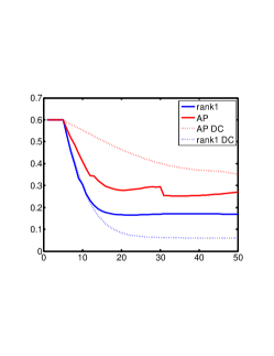
(d) NRMSE $\min_{c^{\ell}}\|c^{\ell}w^{(\ell)}-w_{0}\|/\|w_{0}\|$

(e) True specimen

(f) Recovered specimen

Figure 2: Initial probe, true illumination, final illumination. Convergence with strong DC term (99%) or with DC term removed. test object, reconstruction. Residual disparities are ascribed to global translations between the “true” illumination and image used for simulations. At every illumination update, the center of mass of the illuminations is centered within one neighboring pixel. Further analysis of fractional shifts and aberrations can be performed using the prescription given in marchesiniXRM .

V Acknowledgements

This work is partially supported by the Center for Applied Mathematics for Energy Research Applications (CAMERA), which is a partnership between Basic Energy Sciences (BES) and Advanced Scientific Computing Research (ASRC) at the U.S Department of Energy under contract DE-AC02-05CH11231 (SM).

References

• [1] Brian Abbey, Keith A. Nugent, Garth J. Williams, Jesse N. Clark, Andrew G. Peele, Mark A. Pfeifer, Martin de Jonge, and Ian McNulty. Keyhole coherent diffractive imaging. Nature Physics, 4:394–398, 03 2008.
• [2] D J Batey, D Claus, and J M Rodenburg. Information multiplexing in ptychography. Ultramicroscopy, 138:13–21, 2014.
• [3] Mike Beckers, Tobias Senkbeil, Thomas Gorniak, Klaus Giewekemeyer, Tim Salditt, and Axel Rosenhahn. Drift correction in ptychographic diffractive imaging. Ultramicroscopy, 126(0):44 – 47, 2013.
• [4] H. N. Chapman. Phase-retrieval x-ray microscopy by wigner -distribution deconvolution. Ultramicroscopy, 66:153–172, 1996.
• [5] Siyuan Dong, Radhika Shiradkar, Pariksheet Nanda, and Guoan Zheng. Spectral multiplexing and coherent-state decomposition in fourier ptychographic imaging. Biomedical Optics Express, 5(6):1757–1767, 2014.
• [6] J. R. Fienup, J. C. Marron, T. J. Schulz, and J. H. Seldin. Hubble space telescope characterized by using phase-retrieval algorithms. Appl. Opt., 32(10):1747–1767, Apr 1993.
• [7] James R Fienup. Phase retrieval: Hubble and the James Webb Space Telescope, 2003. Center for Adaptive Optics, 2003 Spring Retreat, San Jose, CA.
• [8] Pierre Godard, Marc Allain, Virginie Chamard, and John Rodenburg. Noise models for low counting rate coherent diffraction imaging. Opt. Express, 20(23):25914–25934, Nov 2012.
• [9] M. Guizar-Sicairos and J. R. Fienup. Phase retrieval with transverse translation diversity: a nonlinear optimization approach. Opt. Express, 16:7264–7278, 2008.
• [10] Manuel Guizar-Sicairos and James R. Fienup. Measurement of coherent x-ray focusedbeams by phase retrieval with transversetranslation diversity. Opt. Express, 17(4):2670–2685, Feb 2009.
• [11] Manuel Guizar-Sicairos, Suresh Narayanan, Aaron Stein, Meredith Metzler, Alec R. Sandy, James R. Fienup, and Kenneth Evans-Lutterodt. Measurement of hard x-ray lens wavefront aberrations using phase retrieval. Applied Physics Letters, 98(11):111108, 2011.
• [12] R. Hegerl and W. Hoppe. Dynamic theory of crystalline structure analysis by electron diffraction in inhomogeneous primary wave field. Berichte Der Bunsen-Gesellschaft Fur Physikalische Chemie, 74:1148, 1970.
• [13] Robert Hesse, D Russell Luke, Shoham Sabach, and Matthew K Tam. Proximal heterogeneous block implicit-explicit method and application to blind ptychographic diffraction imaging. SIAM Journal on Imaging Sciences, 8(1):426–457, 2015.
• [14] Susanne Hönig, Robert Hoppe, Jens Patommel, Andreas Schropp, Sandra Stephan, Sebastian Schöder, Manfred Burghammer, and Christian G. Schroer. Full optical characterization of coherent x-ray nanobeams by ptychographic imaging. Opt. Express, 19(17):16324–16329, Aug 2011.
• [15] W. Hoppe. Beugung im inhomogenen Primärstrahlwellenfeld. I. Prinzip einer Phasenmessung von Elektronenbeungungsinterferenzen. Acta Crystallographica Section A, 25(4):495–501, 1969.
• [16] N. C. Jesse and G. P. Andrew. Simultaneous sample and spatial coherence characterisation using diffractive imaging. Applied Physics Letters, 99(15):154103, 2011.
• [17] C.M. Kewish, P. Thibault, M. Dierolf, O. Bunk, A. Menzel, J. Vila-Comamala, K. Jefimovs, and F. Pfeiffer. Ptychographic characterization of the wavefield in the focus of reflective hard x-ray optics. Ultramicroscopy, 110:325–9, Mar 2010.
• [18] A.M. Maiden, M.J. Humphry, M.C. Sarahan, B. Kraus, and J.M. Rodenburg. An annealing algorithm to correct positioning errors in ptychography. Ultramicroscopy, 120(0):64 – 72, 2012.
• [19] S Marchesini, HN Chapman, A Barty, C Cui, MR Howells, JCH Spence, U Weierstall, and AM Minor. Phase aberrations in diffraction microscopy. IPAP Conf. Series 7 pp.380-382, 2006, arXiv preprint physics/0510033, 2006.
• [20] Stefano Marchesini, Andre Schirotzek, Chao Yang, Hau-tieng Wu, and Filipe Maia. Augmented projections for ptychographic imaging. Inverse Problems, 29(11):115009, 2013.
• [21] Stefano Marchesini, Yu-Chao Tu, and Hau-tieng Wu. Alternating projection, ptychographic imaging and phase synchronization. arXiv preprint arXiv:1402.0550, 2014.
• [22] Joanne Marrison, Lotta Räty, Poppy Marriott, and Peter O’Toole. Ptychography-a label free, high-contrast imaging technique for live cells using quantitative phase information. Scientific reports, 3, 2013.
• [23] J. M. Rodenburg and R. H. T. Bates. The theory of super-resolution electron microscopy via wigner-distribution deconvolution. Phil. Trans. R. Soc. Lond. A, 339:521–553, 1992.
• [24] J. M. Rodenburg and H. M. L. Faulkner. A phase retrieval algorithm for shifting illumination. Appl. Phy. Lett., 85:4795–4797, 2004.
• [25] Andreas Schropp, Robert Hoppe, Vivienne Meier, Jens Patommel, Frank Seiboth, Hae Ja Lee, Bob Nagler, Eric C Galtier, Brice Arnold, Ulf Zastrau, et al. Full spatial characterization of a nanofocused x-ray free-electron laser beam by ptychographic imaging. Scientific reports, 3, 2013.
• [26] John CH Spence. High-resolution electron microscopy, volume 60. Clarendon Press, 2003.
• [27] Marco Stockmar, Peter Cloetens, Irene Zanette, Bjoern Enders, Martin Dierolf, Franz Pfeiffer, and Pierre Thibault. Near-field ptychography: phase retrieval for inline holography using a structured illumination. Scientific reports, 3, 2013.
• [28] P. Thibault, M. Dierolf, O. Bunk, A. Menzel, and F. Pfeiffer. Probe retrieval in ptychographic coherent diffractive imaging. Ultramicroscopy, 109:338–43, Mar 2009.
• [29] P. Thibault, M. Dierolf, A. Menzel, O. Bunk, C. David, and F. Pfeiffer. High-Resolution scanning x-ray diffraction microscopy. Science, 321(5887):379–382, 2008.
• [30] P. Thibault and M. Guizar-Sicairos. Maximum-likelihood refinement for coherent diffractive imaging. New Journal of Physics, 14(6):063004, 2012.
• [31] Samuel T Thurman and James R Fienup. Phase retrieval with signal bias. JOSA A, 26(4):1008–1014, 2009.
• [32] Lei Tian, Xiao Li, Kannan Ramchandran, and Laura Waller. Multiplexed coded illumination for fourier ptychography with an led array microscope. Biomedical Optics Express, 5(7):2376–2389, 2014.
• [33] DJ Vine, GJ Williams, B Abbey, MA Pfeifer, JN Clark, MD De Jonge, I McNulty, AG Peele, and KA Nugent. Ptychographic fresnel coherent diffractive imaging. Physical Review A, 80(6):063823, 2009.
• [34] L. W. Whitehead, G. J. Williams, H. M. Quiney, D. J. Vine, R. A. Dilanian, S. Flewett, K. A. Nugent, A. G. Peele, E. Balaur, and I. McNulty. Diffractive imaging using partially coherent x rays. Phys. Rev. Lett., 103:243902, Dec 2009.
• [35] Antoine Wojdyla, MP Benk, DG Johnson, A Donoghue, and KA Goldberg. Fourier ptychography microscopy with the sharp euv microscope for increased imaging resolution based on illumination diversity. In 2014 International Symposium on Extreme Ultraviolet Lithography, Washington DC, 2014.
• [36] C. Yang, J. Qian, A. Schirotzek, F. Maia, and S. Marchesini. Iterative algorithms for ptychographic phase retrieval. Technical Report 4598E, arXiv:1105.5628, Lawrence Berkeley National Laboratory, 2011.
• [37] Guoan Zheng, Roarke Horstmeyer, and Changhuei Yang. Wide-field, high-resolution fourier ptychographic microscopy. Nature Photonics, 7(9):739–745, 2013.