Abstract

We study the effects of Lepton Flavor Violation (LFV) in the scalar lepton sector of the MSSM on precision observables such as the $W$-boson mass and the effective weak leptonic mixing angle, and on the Higgs-boson mass predictions. The slepton mass matrices are parameterized in a model-independent way by a complete set of dimensionless parameters which we constrain through LFV decay processes and the precision observables. We find regions where both conditions are similarly constraining. The necessary prerequisites for the calculation have been added to FeynArts and FormCalc and are thus publicly available for further studies. The obtained results are available in FeynHiggs.

1 Introduction

Lepton Flavor Violating (LFV) processes provide one of the most interesting probes to physics beyond the Standard Model (SM) of particle physics. All SM interactions preserve lepton flavor number and therefore a measurement of any (charged) LFV process would be an unambiguous signal of physics beyond the SM and provide interesting information on the involved flavor mixing, as well as on the underlying origin for this mixing (for a review see Ref. [1], for instance).

The data from past and ongoing neutrino oscillation experiments, as well as from cosmology and astrophysics, have confirmed that neutrinos have different non-zero masses and that the three neutrino flavors $\nu_{e}$, $\nu_{\mu}$, $\nu_{\tau}$ mix to form three mass eigenstates. This implies non-conservation of lepton flavor, clearly beyond the SM. Thus, lepton-flavor-violating processes are expected in the lepton sector just as quark-flavor-violating processes arise in the quark sector.

Within the Minimal Supersymetric Standard Model (MSSM) [2], LFV can occur in the scalar lepton sector. The most general way to introduce slepton flavor mixing within the MSSM is through the off-diagonal soft-SUSY-breaking parameters (both mass parameters and trilinear couplings) in the slepton sector. The off-diagonality in the slepton mass matrix reflects the misalignment (in flavor space) between lepton and slepton mass matrices, which cannot be diagonalized simultaneously. This misalignment can have various origins; for instance, off-diagonal slepton mass matrix entries can be generated by Renormalization Group Equations running from high energies, where heavy right-handed neutrinos are assumed to be active, down to low energies where LFV processes can occur [3, 4].

In this work we do not investigate the possible dynamical origin of this lepton–slepton misalignment, nor particular predictions for off-diagonal slepton soft-SUSY-breaking mass terms in specific SUSY models, but instead parameterize the slepton mass matrix and explore the phenomenological implications of LFV on various observables.

Specifically, we write the off-diagonal slepton mass matrix elements in terms of a complete set of generic dimensionless parameters $\delta_{\{12,13,23\}}^{\{LL,LR,RL,RR\}}$, where $L,R$ refers to the left-/right-handed SUSY partner of the corresponding leptonic degree of freedom and $1,2,3$ are the involved generation indices, and explore the sensitivity of several precision observables to the $\delta^{AB}_{ij}$’s, extending a program carried out for flavor violation in the scalar quark sector [5].

Besides direct searches, which have not turned up evidence for any additional particles so far, SUSY can also be probed through its effects on precision observables via virtual particles, see Ref. [6] for a review. Electroweak precision observables (EWPO) like the $W$-boson mass or the effective weak leptonic mixing angle have been measured to a very high precision, and the anticipated improved precision in current and future experiments for these observables makes them very sensitive to physics beyond the SM.

Besides EWPO we also explore the effects of LFV on the MSSM Higgs sector, again extending existing analyses on flavor violation in the scalar quark sector [7, 5]. The MSSM Higgs sector consist of two Higgs doublets and predicts five physical Higgs bosons, the light and heavy ${\cal CP}$-even $h$ and $H$, the ${\cal CP}$-odd $A$, and the charged Higgs boson $H^{\pm}$. At tree level the Higgs sector is described with the help of two parameters: the mass of the $A$ boson, $M_{A}$, and $\tan\beta:=v_{2}/v_{1}$, the ratio of the two vacuum expectation values. After the spectacular discovery of a Higgs particle at the LHC, the precision of the measured mass value is already below the GeV level [8, 9], and at a future ILC, a precision even below $\sim 50\,\,\mathrm{MeV}$ is anticipated [10]. We evaluate the effects of LFV on the predictions of the masses of the light and heavy ${\cal CP}$-even Higgs bosons, $M_{h}$ and $M_{H}$, as well as on the charged Higgs-boson mass $M_{H^{\pm}}$. Based on the evaluations in the scalar quark sector [5], theoretical uncertainties from LFV effects on the evaluation of the Higgs-boson masses are substantially larger than the future experimental accuracy could be expected, motivating the analytical calculation of these corrections.

For our calculations we prepared (and thoroughly tested) an add-on model file for FeynArts [11, 12] which adds LFV effects to the existing MSSM model file. No renormalization as in Ref. [13] is included yet (and also not necessary for the present work since the SM is lepton-flavor conserving and hence there is no tree-level contribution). The FormCalc [14] driver files were also modified accordingly. We checked that the LFV Feynman rules yield finite results for all our calculations. The results derived with this setup, the Higgs-boson masses as well as the EWPO, were added to FeynHiggs 2.10.2.

This paper is organized as follows: First we review the main features of the MSSM with general slepton flavor mixing and set the relevant notation for the $\delta^{AB}_{ij}$’s in  Sect. 2. The selection of specific MSSM scenarios as well as their experimental restrictions from LFV processes is presented in Sect. 3. The numerical analysis is given in Sect. 4, showing for the first time the LFV effects on the MSSM Higgs boson masses and on the EWPO. Sect. 5 summarizes our conclusions.

2 Calculational Basis

We work in MSSM scenarios with general flavor mixing in the sleptons. Within these MSSM-FV scenarios, lepton flavor violation is induced by the PMNS matrix of the neutrino sector and transmitted by the small neutrino Yukawa couplings which we ignore here. Flavor mixing in the slepton mass matrix is the main generator of LFV. In the following we give a brief overview about the relevant sectors of the MSSM with LFV.

2.1 Scalar lepton sector with LFV

For the slepton sector of the MSSM including LFV contributions we use the same notation as Ref. [20]. The most general hypothesis for flavor mixing in the slepton sector assumes a non-diagonal mass matrix for both charged sleptons and sneutrinos. For the charged sleptons this is a $6\times 6$ mass matrix since there are six electroweak interaction eigenstates, $\tilde{\ell}_{L,R}$ with $\ell=e,\mu,\tau$, while for the sneutrinos the matrix is only $3\times 3$ corresponding to the three states $\tilde{\nu}_{L}$ with $\nu=\nu_{e},\nu_{\mu},\nu_{\tau}$.

The non-diagonal entries in the $6\times 6$ general matrix for charged sleptons can be described in a model-independent way in terms of a set of dimensionless parameters $\delta^{AB}_{ij}$ ($A,B=L,R$; $i,j=1,2,3$, $i\neq j$), where $L,R$ refer to the left-/right-handed SUSY partners of the corresponding leptonic degrees of freedom, and the indices $i,j$ run over the three generations. These scenarios with general sfermion flavor mixing lead generally to larger LFV rates than in the so-called Minimal Flavor Violation Scenarios, where the mixing is induced exclusively by the Yukawa coupling of the corresponding fermion sector. This is true for both squarks and sleptons but it is obviously of special interest in the slepton case due to the extremely small size of the lepton Yukawa couplings, suppressing LFV processes from this origin. Hence in the present case of slepton mixing we assume that the $\delta^{AB}_{ij}$’s provide the sole source of LFV processes with potentially measurable rates.

The non-diagonal $6\times 6$ slepton mass matrix, which we order here as $(\tilde{e}_{L},\tilde{\mu}_{L},\tilde{\tau}_{L},\tilde{e}_{R},\tilde{\mu}_{R},\tilde{\tau}_{R})$, is usually decomposed into left- and right-handed $3\times 3$ blocks $M^{2}_{\tilde{\ell},AB}$ as

$$\mathcal{M}_{\tilde{\ell}}^{2}=\begin{pmatrix}M^{2}_{\tilde{\ell},LL}&M^{2}_{\tilde{\ell},LR}\\[3.00003pt] M_{\tilde{\ell},LR}^{2\,\dagger}&M^{2}_{\tilde{\ell},RR}\end{pmatrix},$$ (1)

where

$$(M^{2}_{\tilde{\ell},LL})_{ij} =(m^{2}_{\tilde{L}})_{ij}+\left(m_{\ell_{i}}^{2}+(-\tfrac{1}{2}+s_{\mathrm{w}}^{2})M_{Z}^{2}\cos 2\beta\right)\delta_{ij}\,,$$ (2)

$$(M^{2}_{\tilde{\ell},RR})_{ij} =(m^{2}_{\tilde{E}})_{ij}+\left(m_{\ell_{i}}^{2}-s_{\mathrm{w}}^{2}M_{Z}^{2}\cos 2\beta\right)\delta_{ij}\,,$$

$$(M^{2}_{\tilde{\ell},LR})_{ij} =v_{1}\mathcal{A}_{ij}^{\ell}-m_{\ell_{i}}\mu\tan\beta\,\delta_{ij}\,,$$

with flavor indexes $i,j=1,2,3$, $s_{\mathrm{w}}=\sqrt{1-c_{\mathrm{w}}^{2}}$ with $c_{\mathrm{w}}=M_{W}/M_{Z}$, lepton masses $(m_{\ell_{i}})=(m_{e},m_{\mu},m_{\tau})$, and Higgsino mass parameter $\mu$. The off-diagonal elements arise exclusively from the soft SUSY-breaking parameters: the doublet mass parameters $m^{2}_{\tilde{L}}$, the singlet mass parameters $m^{2}_{\tilde{E}}$, and the trilinear couplings $\mathcal{A}^{\ell}$, which are all $3\times 3$ matrices in flavor space.

The sneutrino mass matrix contains only a single $3\times 3$ block (ordered as $(\tilde{\nu}_{eL},\tilde{\nu}_{\mu L},\tilde{\nu}_{\tau L})$) to start with since the singlet components are absent:

$$(\mathcal{M}^{2}_{\tilde{\nu}})_{ij}=(M^{2}_{\tilde{\nu},LL})_{ij}=(m^{2}_{\tilde{L}})_{ij}+\tfrac{1}{2}M_{Z}^{2}\cos 2\beta\delta_{ij}\,.$$ (3)

Note that, due to $SU(2)_{L}$ gauge invariance, the same doublet mass parameters $m^{2}_{\tilde{L}}$ enter the slepton and sneutrino $LL$ mass matrices.

If neutrino masses and neutrino flavor mixings (oscillations) were taken into account, the soft-SUSY-breaking parameters for the sneutrinos would differ from the ones for charged sleptons by a rotation with the PMNS matrix. Taking the neutrino masses and oscillations into account in the SM leads to LFV effects that are extremelly small; for instance, in $\mu\to e\gamma$ they are of ${\cal O}(10^{-47})$ in case of Dirac neutrinos with mass around 1 eV and maximal mixing [1, 21, 22], and of ${\cal O}(10^{-40})$ in case of Majorana neutrinos [1, 22]. Consequently we do not expect large effects from the inclusion of neutrino mass effects here.

The dimensionless parameters $\delta^{AB}_{ij}$ allow for a unified description of the off-diagonal soft-SUSY-breaking parameters to which they are related as follows:

$$m^{2}_{\tilde{L}} =\begin{pmatrix}\vrule width=0.0pt,height=10.76385pt,depth=6.45831ptm^{2}_{\tilde{L}_{1}}&\delta_{12}^{LL}m_{\tilde{L}_{1}}m_{\tilde{L}_{2}}&\delta_{13}^{LL}m_{\tilde{L}_{1}}m_{\tilde{L}_{3}}\\ \vrule width=0.0pt,height=10.76385pt,depth=6.45831pt\delta_{21}^{LL}m_{\tilde{L}_{2}}m_{\tilde{L}_{1}}&m^{2}_{\tilde{L}_{2}}&\delta_{23}^{LL}m_{\tilde{L}_{2}}m_{\tilde{L}_{3}}\\ \vrule width=0.0pt,height=10.76385pt,depth=6.45831pt\delta_{31}^{LL}m_{\tilde{L}_{3}}m_{\tilde{L}_{1}}&\delta_{32}^{LL}m_{\tilde{L}_{3}}m_{\tilde{L}_{2}}&m^{2}_{\tilde{L}_{3}}\end{pmatrix},$$ (4)

$$m^{2}_{\tilde{E}} =\begin{pmatrix}\vrule width=0.0pt,height=10.76385pt,depth=6.45831ptm^{2}_{\tilde{E}_{1}}&\delta_{12}^{RR}m_{\tilde{E}_{1}}m_{\tilde{E}_{2}}&\delta_{13}^{RR}m_{\tilde{E}_{1}}m_{\tilde{E}_{3}}\\ \vrule width=0.0pt,height=10.76385pt,depth=6.45831pt\delta_{21}^{RR}m_{\tilde{E}_{2}}m_{\tilde{E}_{1}}&m^{2}_{\tilde{E}_{2}}&\delta_{23}^{RR}m_{\tilde{E}_{2}}m_{\tilde{E}_{3}}\\ \vrule width=0.0pt,height=10.76385pt,depth=6.45831pt\delta_{31}^{RR}m_{\tilde{E}_{3}}m_{\tilde{E}_{1}}&\delta_{32}^{RR}m_{\tilde{E}_{3}}m_{\tilde{E}_{2}}&m^{2}_{\tilde{E}_{3}}\end{pmatrix},$$ (5)

$$v_{1}\mathcal{A}^{\ell} =\begin{pmatrix}\vrule width=0.0pt,height=10.76385pt,depth=6.45831ptm_{e}A_{e}&\delta_{12}^{LR}m_{\tilde{L}_{1}}m_{\tilde{E}_{2}}&\delta_{13}^{LR}m_{\tilde{L}_{1}}m_{\tilde{E}_{3}}\\ \vrule width=0.0pt,height=10.76385pt,depth=6.45831pt\delta_{21}^{LR}m_{\tilde{L}_{2}}m_{\tilde{E}_{1}}&m_{\mu}A_{\mu}&\delta_{23}^{LR}m_{\tilde{L}_{2}}m_{\tilde{E}_{3}}\\ \vrule width=0.0pt,height=10.76385pt,depth=6.45831pt\delta_{31}^{LR}m_{\tilde{L}_{3}}m_{\tilde{E}_{1}}&\delta_{32}^{LR}m_{\tilde{L}_{3}}m_{\tilde{E}_{2}}&m_{\tau}A_{\tau}\end{pmatrix}.$$ (6)

This parameterization is purely phenomenological and does not rely on any specific assumptions on the origin of the soft-SUSY-breaking parameters.

The next step is to rotate the sleptons and sneutrinos from the electroweak interaction basis into the physical mass eigenstate basis,

$$\begin{pmatrix}\tilde{\ell}_{1}\\ \tilde{\ell}_{2}\\ \tilde{\ell}_{3}\\ \tilde{\ell}_{4}\\ \tilde{\ell}_{5}\\ \tilde{\ell}_{6}\end{pmatrix}=R^{\tilde{\ell}}\begin{pmatrix}\tilde{e}_{L}\\ \tilde{\mu}_{L}\\ \tilde{\tau}_{L}\\ \tilde{e}_{R}\\ \tilde{\mu}_{R}\\ \tilde{\tau}_{R}\end{pmatrix},\qquad\begin{pmatrix}\tilde{\nu}_{1}\\ \tilde{\nu}_{2}\\ \tilde{\nu}_{3}\end{pmatrix}=R^{\tilde{\nu}}\begin{pmatrix}\tilde{\nu}_{eL}\\ \tilde{\nu}_{\mu L}\\ \tilde{\nu}_{\tau L}\end{pmatrix},$$ (7)

where $R^{\tilde{\ell}}$ and $R^{\tilde{\nu}}$ are the unitary matrices resulting from diagonalizing the mass matrices,

$$R^{\tilde{\ell}}\,\mathcal{M}^{2}_{\tilde{\ell}}\,R^{\tilde{\ell}\dagger} =\mathop{\mathrm{diag}}\{m_{\tilde{\ell}_{1}}^{2},m_{\tilde{\ell}_{2}}^{2},m_{\tilde{\ell}_{3}}^{2},m_{\tilde{\ell}_{4}}^{2},m_{\tilde{\ell}_{5}}^{2},m_{\tilde{\ell}_{6}}^{2}\}\,,$$ (8)

$$R^{\tilde{\nu}}\,\mathcal{M}^{2}_{\tilde{\nu}}\,R^{\tilde{\nu}\dagger} =\mathop{\mathrm{diag}}\{m_{\tilde{\nu}_{1}}^{2},m_{\tilde{\nu}_{2}}^{2},m_{\tilde{\nu}_{3}}^{2}\}\,.$$

2.2 Higgs masses and mixing

In this section we shortly review the relevant features of the MSSM Higgs sector at tree-level. Unlike the SM, the MSSM requires two Higgs doublets. The Higgs potential [25]

$$V =m_{1}^{2}|{\cal H}_{1}|^{2}+m_{2}^{2}|{\cal H}_{2}|^{2}-m_{12}^{2}(\epsilon_{ab}{\cal H}_{1}^{a}{\cal H}_{2}^{b}+\mbox{h.c.})+{}$$ (9)

$$\qquad\frac{1}{8}(g_{1}^{2}+g_{2}^{2})\left[|{\cal H}_{1}|^{2}-|{\cal H}_{2}|^{2}\right]^{2}+\frac{1}{2}g_{2}^{2}|{\cal H}_{1}^{{\dagger}}{\cal H}_{2}|^{2}\,,$$

contains $m_{1}$, $m_{2}$, $m_{12}$ as soft-SUSY-breaking parameters; $g_{2},g_{1}$ are the $SU(2)$ and $U(1)$ gauge couplings, and $\epsilon$ is the spinor metric with $\epsilon_{12}=-1$.

The doublet fields $H_{1}$ and $H_{2}$ are decomposed as

$${\cal H}_{1} =\begin{pmatrix}{\cal H}_{1}^{0}\\[2.15277pt] {\cal H}_{1}^{-}\end{pmatrix}=\begin{pmatrix}v_{1}+\frac{1}{\sqrt{2}}(\phi_{1}^{0}-i\chi_{1}^{0})\\[2.15277pt] -\phi_{1}^{-}\end{pmatrix},$$ (10)

$${\cal H}_{2} =\begin{pmatrix}{\cal H}_{2}^{+}\\[2.15277pt] {\cal H}_{2}^{0}\end{pmatrix}=\begin{pmatrix}\phi_{2}^{+}\\[2.15277pt] v_{2}+\frac{1}{\sqrt{2}}(\phi_{2}^{0}+i\chi_{2}^{0})\end{pmatrix}.$$

The Higgs potential is thus characterized at tree level by only two independent parameters: $\tan\beta=v_{2}/v_{1}$ and $M_{A}^{2}=-m_{12}^{2}(\tan\beta+\cot\beta)$, where $M_{A}$ is the mass of the ${\cal CP}$-odd Higgs boson $A$.

The bilinear part of the Higgs potential is diagonalized by orthogonal transformations

$$\begin{pmatrix}H\\[2.15277pt] h\end{pmatrix} =\begin{pmatrix}\cos\alpha&\sin\alpha\\[2.15277pt] -\sin\alpha&\cos\alpha\end{pmatrix}\begin{pmatrix}\phi_{1}^{0}\\[2.15277pt] \phi_{2}^{0}\end{pmatrix},$$ (11)

$$\begin{pmatrix}G\\[2.15277pt] A\end{pmatrix} =\begin{pmatrix}\cos\beta&\sin\beta\\[2.15277pt] -\sin\beta&\cos\beta\end{pmatrix}\begin{pmatrix}\chi_{1}^{0}\\[2.15277pt] \chi_{2}^{0}\end{pmatrix},$$ (12)

$$\begin{pmatrix}G^{\pm}\\[2.15277pt] H^{\pm}\end{pmatrix} =\begin{pmatrix}\cos\beta&\sin\beta\\[2.15277pt] -\sin\beta&\cos\beta\end{pmatrix}\begin{pmatrix}\phi_{1}^{\pm}\\[2.15277pt] \phi_{2}^{\pm}\end{pmatrix}.$$ (13)

where the tree-level mixing angle $\alpha$ is given by

$$\alpha=\arctan\left[\frac{-(M_{A}^{2}+M_{Z}^{2})\sin\beta\cos\beta}{M_{Z}^{2}\cos^{2}\beta+M_{A}^{2}\sin^{2}\beta-m^{2}_{h,{\rm tree}}}\right],\quad-\frac{\pi}{2}<\alpha<0\,.$$ (14)

The Higgs spectrum is thus:

$$\mbox{2 neutral bosons},\,{\cal CP}=+1 :\quad h,\ H,$$

$$\mbox{1 neutral boson},\,{\cal CP}=-1 :\quad A,$$

2 charged bosons $$:\quad H^{+},\ H^{-},$$

3 unphysical Goldstone bosons $$:\quad G,\ G^{+},\ G^{-}.$$

At tree level the neutral ${\cal CP}$-even Higgs-boson masses are determined from

$$M_{\text{Higgs}}^{2,\text{tree}}=\begin{pmatrix}M_{A}^{2}\sin^{2}\beta+M_{Z}^{2}\cos^{2}\beta&-(M_{A}^{2}+M_{Z}^{2})\sin\beta\cos\beta\\ -(M_{A}^{2}+M_{Z}^{2})\sin\beta\cos\beta&M_{A}^{2}\cos^{2}\beta+M_{Z}^{2}\sin^{2}\beta\end{pmatrix}\overset{\hbox to0.0pt{\large$\circlearrowleft$\hss}\,\,\raise 1.20448pt\hbox{\scriptsize$\alpha$}~{}}{\longrightarrow}\begin{pmatrix}m_{H,\text{tree}}^{2}&0\\ 0&m_{h,\text{tree}}^{2}\end{pmatrix}.$$ (15)

which yields

$$(m_{H,h}^{2})_{\text{tree}}=\frac{1}{2}\left[M_{A}^{2}+M_{Z}^{2}\pm\sqrt{(M_{A}^{2}+M_{Z}^{2})^{2}-4M_{Z}^{2}M_{A}^{2}\cos^{2}2\beta}\right]$$ (16)

and the charged Higgs-boson mass is given by

$$m^{2}_{H^{\pm},\text{tree}}=M_{A}^{2}+M_{W}^{2}\,.$$ (17)

2.3 Calculation of higher-order corrections in the Higgs sector

We briefly review the procedure of Refs. [18, 26] for the computation of one-loop corrections to the Higgs-boson masses. The parameters appearing in the Higgs potential, Eq. (9), are renormalized as follows:

$$M_{Z}^{2} \to M_{Z}^{2}+\delta M_{Z}^{2}\,, T_{h} \to T_{h}+\delta T_{h}\,,$$ (18)

$$M_{W}^{2} \to M_{W}^{2}+\delta M_{W}^{2}\,, T_{H} \to T_{H}+\delta T_{H}\,,$$

$$M_{\text{Higgs}}^{2} \to M_{\text{Higgs}}^{2}+\delta M_{\text{Higgs}}^{2}\,,\quad \tan\beta \to\tan\beta\,(1+\delta\!\tan\!\beta\,)\,.$$

$M_{\text{Higgs}}^{2}$ denotes the tree-level Higgs-boson mass matrix of Eq. (15), and $T_{h}$ and $T_{H}$ are the tree-level tadpoles, i.e. the terms linear in $h$ and $H$ in the Higgs potential.

In the ${\cal CP}$-even sector the mass and field renormalization can be set up symmetrically,

$$\delta M_{\rm Higgs}^{2}=\begin{pmatrix}\delta m_{h}^{2}&\delta m_{hH}^{2}\\[5.0pt] \delta m_{hH}^{2}&\delta m_{H}^{2}\end{pmatrix},\qquad\begin{pmatrix}h\\[5.0pt] H\end{pmatrix}\to\begin{pmatrix}1+\tfrac{1}{2}\delta Z_{hh}&\tfrac{1}{2}\delta Z_{hH}\\[5.0pt] \tfrac{1}{2}\delta Z_{hH}&1+\tfrac{1}{2}\delta Z_{HH}\end{pmatrix}\begin{pmatrix}h\\[5.0pt] H\end{pmatrix}.$$ (19)

The renormalized self-energies $\hat{\Sigma}(p^{2})$ are expressed through the unrenormalized self-energies $\Sigma(p^{2})$, the field renormalization constants, and the mass counter-terms as follows:

$$\hat{\Sigma}_{hh}(p^{2}) =\Sigma_{hh}(p^{2})+\delta Z_{hh}(p^{2}-m_{h,{\rm tree}}^{2})-\delta m_{h}^{2}\,,$$ (20)

$$\hat{\Sigma}_{hH}(p^{2}) =\Sigma_{hH}(p^{2})+\delta Z_{hH}(p^{2}-\tfrac{1}{2}(m_{h,{\rm tree}}^{2}+m_{H,{\rm tree}}^{2}))-\delta m_{hH}^{2}\,,$$

$$\hat{\Sigma}_{HH}(p^{2}) =\Sigma_{HH}(p^{2})+\delta Z_{HH}(p^{2}-m_{H,{\rm tree}}^{2})-\delta m_{H}^{2}\,.$$

Inserting the renormalization transformation into the Higgs mass terms gives the following Higgs-mass counter-terms:

$$\delta m_{h}^{2} =\delta M_{A}^{2}\cos^{2}(\alpha-\beta)+\delta M_{Z}^{2}\sin^{2}(\alpha+\beta)+{}$$ (21)

$$\qquad\tfrac{e}{2M_{Z}s_{\mathrm{w}}c_{\mathrm{w}}}(\delta T_{H}\cos(\alpha-\beta)\sin^{2}(\alpha-\beta)+\delta T_{h}\sin(\alpha-\beta)(1+\cos^{2}(\alpha-\beta)))+{}$$

$$\qquad\delta\!\tan\!\beta\,\sin\beta\,\cos\beta\,(M_{A}^{2}\sin 2(\alpha-\beta)+M_{Z}^{2}\sin 2(\alpha+\beta))\,,$$

$$\delta m_{hH}^{2} =\tfrac{1}{2}(\delta M_{A}^{2}\sin 2(\alpha-\beta)-\delta M_{Z}^{2}\sin 2(\alpha+\beta))+{}$$

$$\qquad\tfrac{e}{2M_{Z}s_{\mathrm{w}}c_{\mathrm{w}}}(\delta T_{H}\sin^{3}(\alpha-\beta)-\delta T_{h}\cos^{3}(\alpha-\beta))-{}$$

$$\qquad\delta\!\tan\!\beta\,\sin\beta\,\cos\beta\,(M_{A}^{2}\cos 2(\alpha-\beta)+M_{Z}^{2}\cos 2(\alpha+\beta))\,,$$

$$\delta m_{H}^{2} =\delta M_{A}^{2}\sin^{2}(\alpha-\beta)+\delta M_{Z}^{2}\cos^{2}(\alpha+\beta)-{}$$

$$\qquad\tfrac{e}{2M_{Z}s_{\mathrm{w}}c_{\mathrm{w}}}(\delta T_{H}\cos(\alpha-\beta)(1+\sin^{2}(\alpha-\beta))+\delta T_{h}\sin(\alpha-\beta)\cos^{2}(\alpha-\beta))-{}$$

$$\qquad\delta\!\tan\!\beta\,\sin\beta\,\cos\beta\,(M_{A}^{2}\sin 2(\alpha-\beta)+M_{Z}^{2}\sin 2(\alpha+\beta))\,.$$

We give the Higgs doublets one renormalization constant each,

$${\cal H}_{1}\to(1+\tfrac{1}{2}\delta Z_{{\cal H}_{1}}){\cal H}_{1}\,,\quad{\cal H}_{2}\to(1+\tfrac{1}{2}\delta Z_{{\cal H}_{2}}){\cal H}_{2}\,,$$ (22)

which leads to the field renormalization constants

$$\delta Z_{hh} =\sin^{2}\!\alpha\,\delta Z_{{\cal H}_{1}}+\cos^{2}\!\alpha\,\delta Z_{{\cal H}_{2}}\,,$$ (23)

$$\delta Z_{hH} =\sin\alpha\,\cos\alpha\,(\delta Z_{{\cal H}_{2}}-\delta Z_{{\cal H}_{1}})\,,$$

$$\delta Z_{HH} =\cos^{2}\!\alpha\,\delta Z_{{\cal H}_{1}}+\sin^{2}\!\alpha\,\delta Z_{{\cal H}_{2}}\,.$$

The counter-term for $\tan\beta$ can be expressed in terms of the vacuum expectation values as

$$\delta\tan\beta=\frac{1}{2}\left(\delta Z_{{\cal H}_{2}}-\delta Z_{{\cal H}_{1}}\right)+\frac{\delta v_{2}}{v_{2}}-\frac{\delta v_{1}}{v_{1}}\,,$$ (24)

where the $\delta v_{i}$ are the renormalization constants of the $v_{i}$:

$$v_{1}\to\left(1+\delta Z_{{\cal H}_{1}}\right)\left(v_{1}+\delta v_{1}\right),\quad v_{2}\to\left(1+\delta Z_{{\cal H}_{2}}\right)\left(v_{2}+\delta v_{2}\right).$$ (25)

It can be shown that the divergent parts of $\delta v_{1}/v_{1}$ and $\delta v_{2}/v_{2}$ are equal [27, 26], thus we set $\delta v_{2}/v_{2}-\delta v_{1}/v_{1}$ to zero.

In the charged Higgs sector, the renormalized self-energy is written similarly as

$$\hat{\Sigma}_{H^{-}H^{+}}(p^{2})=\Sigma_{H^{-}H^{+}}(p^{2})+\delta Z_{H^{-}H^{+}}(p^{2}-m^{2}_{H^{\pm},\text{tree}})-\delta m_{H^{\pm}}^{2},$$ (26)

where

$$\delta m_{H^{\pm}}^{2} =\delta M_{A}^{2}+\delta M_{W}^{2}\,,$$ (27)

$$\delta Z_{H^{-}H^{+}} =\sin^{2}\beta\,\delta Z_{{\cal H}_{1}}+\cos^{2}\beta\,\delta Z_{{\cal H}_{2}}\,.$$ (28)

We apply on-shell conditions for the masses

$$\delta M_{Z}^{2}=\mathop{\mathrm{Re}}\Sigma_{ZZ}^{T}(M_{Z}^{2})\,,\quad\delta M_{W}^{2}=\mathop{\mathrm{Re}}\Sigma_{WW}^{T}(M_{W}^{2})\,,\quad\delta M_{A}^{2}=\mathop{\mathrm{Re}}\Sigma_{AA}(M_{A}^{2})\,.$$ (29)

Since the tadpole coefficients are chosen to vanish in all orders, their counter-terms follow from $T_{\{h,H\}}+\delta T_{\{h,H\}}=0$:

$$\delta T_{h}=-T_{h},\quad\delta T_{H}=-T_{H}\,.$$ (30)

$\overline{\rm{DR}}$ renormalization is the most convenient choice for the remaining renormalization constants

$$\delta Z_{{\cal H}_{1}} =\delta Z_{{\cal H}_{1}}^{\overline{\rm{DR}}}=-\left[\mathop{\mathrm{Re}}\Sigma^{\prime}_{HH\;|\alpha=0}\right]^{\rm div},$$ (31)

$$\delta Z_{{\cal H}_{2}} =\delta Z_{{\cal H}_{2}}^{\overline{\rm{DR}}}=-\left[\mathop{\mathrm{Re}}\Sigma^{\prime}_{hh\;|\alpha=0}\right]^{\text{div}},$$

$$\delta\!\tan\!\beta =\frac{1}{2}(\delta Z_{{\cal H}_{2}}-\delta Z_{{\cal H}_{1}})=\delta\!\tan\!\beta\,^{\overline{\rm{DR}}}\,.$$

We choose a renormalization scale of $\mu_{\overline{\mathrm{DR}}}=m_{t}$ in all numerical evaluations.

Finally, in the Feynman-diagrammatic approach we are following here, the higher-order-corrected ${\cal CP}$-even Higgs-boson masses are derived by finding the poles of the $(h,H)$-propagator matrix. The inverse of this matrix is

$$\bigl{(}\Delta_{\text{Higgs}}\bigr{)}^{-1}=-\mathrm{i}\begin{pmatrix}p^{2}-m_{H,{\rm tree}}^{2}+\hat{\Sigma}_{HH}(p^{2})&\hat{\Sigma}_{hH}(p^{2})\\ \hat{\Sigma}_{hH}(p^{2})&p^{2}-m_{h,{\rm tree}}^{2}+\hat{\Sigma}_{hh}(p^{2})\end{pmatrix}.$$ (32)

Determining its poles is thus equivalent to solving the equation

$$\left[p^{2}-m_{h,{\rm tree}}^{2}+\hat{\Sigma}_{hh}(p^{2})\right]\left[p^{2}-m_{H,{\rm tree}}^{2}+\hat{\Sigma}_{HH}(p^{2})\right]-\left[\hat{\Sigma}_{hH}(p^{2})\right]^{2}=0\,.$$ (33)

The corrected charged Higgs mass is analogously derived as the position of the pole of the charged-Higgs propagator,

$$p^{2}-m^{2}_{H^{\pm},\text{tree}}+\hat{\Sigma}_{H^{-}H^{+}}(p^{2})=0\,.$$ (34)

We calculated the LFV contribution originating from the mixing in the slepton sector in a model-independent approach to the Higgs-boson masses. The present experimental uncertainty at the LHC for $M_{h}$, the mass of the light neutral Higgs boson, is about $350\,\,\mathrm{MeV}$ [8, 9]. This can possibly be reduced by about 50% at the LHC and below the level of $\sim 50\,\,\mathrm{MeV}$ at the ILC [10]. Similarly, for the masses of the heavy neutral Higgs $M_{H}$ and charged Higgs boson $M_{H^{\pm}}$, an uncertainity at the $1\%$ level could be expected at the LHC [28]. This sets the goal for the theoretical uncertainty, which should be reduced to the same (or higher) level of accuracy.

The generic Feynman diagrams for the one-loop Higgs-boson self-energies relevant for our work are shown in Fig. 1. The diagrams were generated with FeynArts and further evaluated using FormCalc, see Sect. 2.5.

Figure 1: Generic Feynman diagrams for the Higgs-boson self-energies and tadpoles. $\phi$ denotes any of the Higgs bosons, $h$, $H$, $A$ or $H^{\pm}$; $\ell$ stands for $e,\mu,\tau$; $\tilde{\ell}_{x}$ are the six mass eigenstates of charged sleptons, and $\tilde{\nu}_{x}$ are the three sneutrino states $\tilde{\nu}_{e}$, $\tilde{\nu}_{\mu}$, $\tilde{\nu}_{\tau}$.

2.4 Calculation of EWPO

EWPO that are known with an accuracy at the per-mille level or better have the potential to allow a discrimination between quantum effects of the SM and SUSY models, see Ref. [6] for a review. Examples are the $W$-boson mass $M_{W}$ and the $Z$-boson observables, such as the effective leptonic weak mixing angle $\sin^{2}\theta_{\mathrm{eff}}$, whose present experimental uncertainities are [29]

$$\delta M_{W}^{\text{exp,today}}\sim 15\,\,\mathrm{MeV},\quad\delta\sin^{2}\theta_{\mathrm{eff}}^{\text{exp,today}}\sim 15\times 10^{-5}\,,$$ (35)

The experimental uncertanity will further be reduced [30] to

$$\delta M_{W}^{\text{exp,future}}\sim 4\,\,\mathrm{MeV},\quad\delta\sin^{2}\theta_{\mathrm{eff}}^{\text{exp,future}}\sim 1.3\times 10^{-5}\,,$$ (36)

at the ILC and at the GigaZ option of the ILC, respectively.

The $W$-boson mass can be evaluated from

$$M_{W}^{2}\left(1-\frac{M_{W}^{2}}{M_{Z}^{2}}\right)=\frac{\pi\alpha}{\sqrt{2}G_{\mu}}(1+\Delta r)$$ (37)

where $\alpha$ is the fine-structure constant and $G_{\mu}$ the Fermi constant. This relation arises from comparing the prediction for muon decay with the experimentally precisely known Fermi constant. The one-loop contributions to $\Delta r$ can be written as

$$\Delta r=\Delta\alpha-\frac{c_{\mathrm{w}}^{2}}{s_{\mathrm{w}}^{2}}\Delta\rho+(\Delta r)_{\text{rem}},$$ (38)

where $\Delta\alpha$ is the shift in the fine-structure constant due to the light fermions of the SM, $\Delta\alpha\propto\log(M_{Z}/m_{f})$, and $\Delta\rho$ is the leading contribution to the $\rho$ parameter [31] from (certain) fermion and sfermion loops. The remainder part $(\Delta r)_{\text{rem}}$ contains in particular the contributions from the Higgs sector.

The effective leptonic weak mixing angle at the $Z$-boson resonance, $\sin^{2}\theta_{\mathrm{eff}}$, is defined through the vector and axial-vector couplings ($g_{\text{V}}^{\ell}$ and $g_{\text{A}}^{\ell}$) of leptons ($\ell$) to the $Z$ boson, measured at the $Z$-boson pole. If this vertex is written as $i\bar{\ell}\gamma^{\mu}(g_{\text{V}}^{\ell}-g_{\text{A}}^{\ell}\gamma_{5})\ell Z_{\mu}$ then

$$\sin^{2}\theta_{\mathrm{eff}}=\frac{1}{4}\left(1-\mathop{\mathrm{Re}}\frac{g_{\text{V}}^{\ell}}{g_{\text{A}}^{\ell}}\right)\,.$$ (39)

At tree level this coincides with the sine of the weak mixing angle, $\sin^{2}\theta_{\text{W}}=1-M_{W}^{2}/M_{Z}^{2}$, in the on-shell scheme. Loop corrections enter through higher-order contributions to $g_{\text{V}}^{\ell}$ and $g_{\text{A}}^{\ell}$.

Both of these (pseudo-)observables are affected by shifts in the quantity $\Delta\rho$ according to

$$\Delta M_{W}\approx\frac{M_{W}}{2}\frac{c_{\mathrm{w}}^{2}}{c_{\mathrm{w}}^{2}-s_{\mathrm{w}}^{2}}\Delta\rho\,,\quad\Delta\sin^{2}\theta_{\mathrm{eff}}\approx-\frac{c_{\mathrm{w}}^{2}s_{\mathrm{w}}^{2}}{c_{\mathrm{w}}^{2}-s_{\mathrm{w}}^{2}}\Delta\rho\,.$$ (40)

The quantity $\Delta\rho$ is defined by the relation

$$\Delta\rho=\frac{\Sigma_{Z}^{\text{T}}(0)}{M_{Z}^{2}}-\frac{\Sigma_{W}^{\text{T}}(0)}{M_{W}^{2}}$$ (41)

with the unrenormalized transverse parts of the $Z$- and $W$-boson self-energies at zero momentum, $\Sigma_{Z,W}^{\text{T}}(0)$. It represents the leading universal corrections to the electroweak precision observables induced by mass splitting between partners in isospin doublets [31]. Consequently, it is sensitive to the mass-splitting effects induced by non-minimal flavour mixing.

Beyond the $\Delta\rho$ approximation, the shifts in $M_{W}$ and $\sin^{2}\theta_{\mathrm{eff}}$ originate from the complete sfermion contributions to the quantity $\Delta r$ and to other combinations of the various vector-boson self-energies. It has been numerically verified that $\Delta\rho$ yields an excellent approximation for the full calculation in the case of NMFV effects [6, 7], however.

We calculated the LFV contribution to the above-mentioned observables entering the $Z$- and $W$-boson self-energies at the one-loop level through the $\rho$-parameter. The generic Feynman diagrams contributing to our calculation are shown in Fig. 2. The diagrams were generated with FeynArts and further evaluated using FormCalc, see Sect. 2.5. The resulting evaluation of $\Delta\rho$ has been made publicly available in FeynHiggs. Using Eq. (40) the shifts in $M_{W}$ and $\sin^{2}\theta_{\mathrm{eff}}$ induced by LFV have been evaluated, see Sect. 4.

Figure 2: Generic Feynman diagrams for the $W$- and $Z$-boson self-energies containing sleptons in loops. The six mass eigenstates of charged sleptons are denoted by $\tilde{\ell}_{x}$, and $\tilde{\nu}_{x}$ stands for the three sneutrino states $\tilde{\nu}_{e}$, $\tilde{\nu}_{\mu}$, $\tilde{\nu}_{\tau}$.

2.5 Changes in FeynArts, FormCalc, and FeynHiggs

FeynArts[11] and FormCalc[14] provide a high level of automation for perturbative calculations up to one loop. This is particularly important for models with a large particle content such as the MSSM [12]. Here we briefly describe the recent extension of the implementation of the MSSM in these packages to include LFV. Details on the previous inclusion of NMFV can be found in Refs. [11, 37]. This involves firstly the modification of the slepton couplings in the existing FeynArts model file for the MSSM and secondly the corresponding initialization routines for the slepton masses and mixings, i.e. the $6\times 6$ and $3\times 3$ diagonalization of the mass matrices in FormCalc.

2.5.1 FeynArts Model File

FeynArts’ add-on model file FV.mod applies algebraic substitutions to the Feynman rules of MSSM.mod to upgrade minimal to non-minimal flavor mixing in the sfermion sector. The original version modified only the squark sector, i.e. NMFV, and needed to be generalized to include LFV. We solved this by allowing the user to choose which sfermion types to introduce non-minimal mixing for through the variable $FV (set before model initialization, of course). For example,

  $FV = {11, 12, 13, 14};
  InsertFields[..., Model -> {MSSM, FV}]

sets non-minimal mixing for all four sfermion types, with 11 = $\tilde{\nu}$, 12 = $\tilde{\ell}$, 13 = $\tilde{u}$, and 14 = $\tilde{d}$ as usual in MSSM.mod. For compatibility with the old NMFV-only version, the default is $FV = {13, 14}.

FV.mod introduces the following new quantities:

UASf[$s_{1}$,$s_{2}$,$t$]	the slepton mixing matrix $R$, where
	$s_{1},s_{2}=1\dots 6$,
	$t=1\,(\tilde{\nu}\/),2\,(\tilde{\ell}\/),3\,(\tilde{u}\/),4\,(\tilde{d}\/)$,
MASf[$s$,$t$]	the slepton masses, where
	$s=1\dots 6$,
	$t=1\,(\tilde{\nu}\/),2\,(\tilde{\ell}\/),3\,(\tilde{u}\/),4\,(\tilde{d}\/)$.

Entries $4\dots 6$ are unused for the sneutrino.

2.5.2 Model Initialization in FormCalc

The initialization of the generalized slepton-mixing parameters MASf and UASf is already built into FormCalc’s regular MSSM model-initialization file model_mssm.F but not turned on by default. It must be enabled by adjusting the FV preprocessor flag in run.F:

   #define FV 2

where 2 is the lowest sfermion type $t$ for which flavor violation is enabled, i.e. $\tilde{\ell}$.

The flavor-violating parameters $\delta^{AB}_{ij}$ are represented in FormCalc by the deltaSf matrix:

double complex deltaSf($s_{1}$,$s_{2}$,$t$)	the matrix $(\delta_{t})_{s_{1}s_{2}}$, where
	$s_{1},s_{2}=1\dots 6$ ($1\dots 3$ for $\tilde{\nu}$),
	$t=2\,(\tilde{\ell}\/),3\,(\tilde{u}\/),4\,(\tilde{d}\/)$.

Since $\delta$ is an Hermitian matrix, only the entries above the diagonal are considered. The $\delta^{AB}_{ij}$ are located at the following places in the matrix $\delta$:

$$\left(\begin{array}[]{ccc|ccc}\vrule width=0.0pt,height=10.76385pt,depth=6.45831pt~{}\cdot{}&\delta^{LL}_{12}&\delta^{LL}_{13}&\vrule width=0.0pt,height=10.76385pt,depth=6.45831pt~{}\cdot{}&\delta^{LR}_{12}&\delta^{LR}_{13}\\ \vrule width=0.0pt,height=10.76385pt,depth=6.45831pt~{}\cdot{}&\vrule width=0.0pt,height=10.76385pt,depth=6.45831pt~{}\cdot{}&\delta^{LL}_{23}&\delta^{RL*}_{12}&\vrule width=0.0pt,height=10.76385pt,depth=6.45831pt~{}\cdot{}&\delta^{LR}_{23}\\ \vrule width=0.0pt,height=10.76385pt,depth=6.45831pt~{}\cdot{}&\vrule width=0.0pt,height=10.76385pt,depth=6.45831pt~{}\cdot{}&\vrule width=0.0pt,height=10.76385pt,depth=6.45831pt~{}\cdot{}&\delta^{RL*}_{13}&\delta^{RL*}_{23}&\vrule width=0.0pt,height=10.76385pt,depth=6.45831pt~{}\cdot{}\\ \hline\cr\vrule width=0.0pt,height=10.76385pt,depth=6.45831pt~{}\cdot{}&\vrule width=0.0pt,height=10.76385pt,depth=6.45831pt~{}\cdot{}&\vrule width=0.0pt,height=10.76385pt,depth=6.45831pt~{}\cdot{}&\vrule width=0.0pt,height=10.76385pt,depth=6.45831pt~{}\cdot{}&\delta^{RR}_{12}&\delta^{RR}_{13}\\ \vrule width=0.0pt,height=10.76385pt,depth=6.45831pt~{}\cdot{}&\vrule width=0.0pt,height=10.76385pt,depth=6.45831pt~{}\cdot{}&\vrule width=0.0pt,height=10.76385pt,depth=6.45831pt~{}\cdot{}&\vrule width=0.0pt,height=10.76385pt,depth=6.45831pt~{}\cdot{}&\vrule width=0.0pt,height=10.76385pt,depth=6.45831pt~{}\cdot{}&\delta^{RR}_{23}\\ \vrule width=0.0pt,height=10.76385pt,depth=6.45831pt~{}\cdot{}&\vrule width=0.0pt,height=10.76385pt,depth=6.45831pt~{}\cdot{}&\vrule width=0.0pt,height=10.76385pt,depth=6.45831pt~{}\cdot{}&\vrule width=0.0pt,height=10.76385pt,depth=6.45831pt~{}\cdot{}&\vrule width=0.0pt,height=10.76385pt,depth=6.45831pt~{}\cdot{}&\vrule width=0.0pt,height=10.76385pt,depth=6.45831pt~{}\cdot{}\end{array}\right)$$

The trilinear couplings $A_{f}$ acquire non-zero off-diagonal entries in the presence of LFV through the relations

$$m_{f,i}(A_{f})_{ij}=(M_{\tilde{f},LR}^{2})_{ij}\,,\quad i,j=1\dots 3\,,$$ (42)

see Eq. (2). These off-diagonal trilinear couplings (and hence the $\delta$’s) appear directly in the Higgs–slepton–slepton couplings, whereas all other effects are mediated through the masses and mixings.

The described changes are contained in FeynArts 3.9 and FormCalc 8.4, which are publicly available from feynarts.de.

2.5.3 Inclusion of LFV into FeynHiggs

As discussed above, the new corrections to the (renormalized) Higgs-boson self-energies (and thus to the Higgs-boson masses), as well as to $\Delta\rho$ (and thus to $M_{W}$ and $\sin^{2}\theta_{\mathrm{eff}}$) have been included in FeynHiggs [15, 16, 17, 18, 19].

The corrections are activated by setting one or more of the $\delta^{AB}_{ij}$ to non-zero values. All $\delta^{AB}_{ij}$ that are not set are assumed to be zero. The non-zero value can be set in three ways:

• by including them in the input file, e.g.

  deltaLLL23    0.1

  where the general format of the identifier is

  delta$F$$XY$$ij$, $F$ = L,E,Q,U,D, $XY$ = LL,LR,RL,RR, $ij$ = 12,23,13

• by calling the subroutine FHSetLFV(…) from your Fortran/C/C++ code.

• by calling the routine FHSetLFV[…] from your Mathematica code.

The detailed invocation of FHSetLFV is given in the corresponding man page included in the FeynHiggs distribution. The LFV corrections are included starting from FeynHiggs version 2.10.2, available from feynhiggs.de.

3 Selection of Input Parameters

3.1 MSSM scenarios

For the following numerical analysis we chose the MSSM parameter sets of Ref. [20]. This framework contains six specific points S1…S6 in the MSSM parameter space, all of which are well compatible with present data, including recent LHC searches and the measurements of the muon anomalous magnetic moment. The values of the various MSSM parameters as well as the values of the predicted MSSM mass spectra are summarized in Tab. 1. They were evaluated with the program FeynHiggs [15, 16, 17, 18, 19].

For simplicity, and to reduce the number of independent MSSM input parameters, we assume equal soft masses for the sleptons of the first and second generations (similarly for the squarks), and for the left and right slepton sectors (similarly for the squarks). We choose equal trilinear couplings for the stop and sbottom squarks and for the sleptons consider only the stau trilinear coupling; the others are set to zero. We assume an approximate GUT relation for the gaugino soft-SUSY-breaking parameters. The pseudoscalar Higgs mass $M_{A}$ and the $\mu$ parameter are taken as independent input parameters. In summary, the six points S1…S6 are defined in terms of the following subset of ten input MSSM parameters:

$$m_{\tilde{L}_{1}}=m_{\tilde{L}_{2}}\,, m_{\tilde{L}_{3}}\,, (\text{with~{}}m_{\tilde{L}_{i}}=m_{\tilde{E}_{i}},\ i=1,2,3)$$

$$m_{\tilde{Q}_{1}}=m_{\tilde{Q}_{2}} m_{\tilde{Q}_{3}}\,, (\text{with~{}}m_{\tilde{Q}_{i}}=m_{\tilde{U}_{i}}=m_{\tilde{D}_{i}},\ i=1,2,3)$$

$$A_{t}=A_{b}\,, A_{\tau}\,,$$

$$M_{2}=2M_{1}=M_{3}/4\,, \mu\,,$$

$$M_{A}\,, \tan\beta\,.$$

Table 1: Selected points in the MSSM parameter space (upper part) and their corresponding spectra (lower part). All dimensionful quantities are in GeV.

S1 S2 S3 S4 S5 S6 $m_{\tilde{L}_{1,2}}$ 500 750 1000 800 500 1500 $m_{\tilde{L}_{3}}$ 500 750 1000 500 500 1500 $M_{2}$ 500 500 500 500 750 300 $A_{\tau}$ 500 750 1000 500 0 1500 $\mu$ 400 400 400 400 800 300 $\tan\beta$ 20 30 50 40 10 40 $M_{A}$ 500 1000 1000 1000 1000 1500 $m_{\tilde{Q}_{1,2}}$ 2000 2000 2000 2000 2500 1500 $m_{\tilde{Q}_{3}}$ 2000 2000 2000 500 2500 1500 $A_{t}$ 2300 2300 2300 1000 2500 1500 $m_{\tilde{\ell}_{1\dots 6}}$ 489–515 738–765 984–1018 474–802 488–516 1494–1507 $m_{\tilde{\nu}_{1\dots 3}}$ 496 747 998 496–797 496 1499 $m_{{\tilde{\chi}}_{1,2}^{\pm}}$ 375–531 376–530 377–530 377–530 710–844 247–363 $m_{{\tilde{\chi}}^{0}_{1\dots 4}}$ 244–531 245–531 245–530 245–530 373–844 145–363 $M_{h}$ 126.6 127.0 127.3 123.1 123.8 125.1 $M_{H}$ 500 1000 999 1001 1000 1499 $M_{A}$ 500 1000 1000 1000 1000 1500 $M_{H^{\pm}}$ 507 1003 1003 1005 1003 1502 $m_{\tilde{u}_{1\dots 6}}$ 1909–2100 1909–2100 1908–2100 336–2000 2423–2585 1423–1589 $m_{\tilde{d}_{1\dots 6}}$ 1997–2004 1994–2007 1990–2011 474–2001 2498–2503 1492–1509 $m_{\tilde{g}}$ 2000 2000 2000 2000 3000 1200

The specific values of these ten MSSM parameters in Tab. 1 are chosen to provide different patterns in the various sparticle masses, but all leading to rather heavy spectra and thus naturally in agreement with the absence of SUSY signals at the LHC. In particular, all points lead to rather heavy squarks and gluinos above $1200\,\,\mathrm{GeV}$ and heavy sleptons above $500\,\,\mathrm{GeV}$ (where the LHC limits would also permit substantially lighter sleptons). The values of $M_{A}$ within the interval $(500,1500)\,\,\mathrm{GeV}$, $\tan\beta$ within the interval $(10,50)$ and a large $A_{t}$ within $(1000,2500)\,\,\mathrm{GeV}$ are fixed such that a light Higgs boson $h$ within the LHC-favoured range $(123,127)\,\,\mathrm{GeV}$ is obtained.

The large values of $M_{A}\geqslant 500$ GeV place the Higgs sector of our scenarios in the so-called decoupling regime[32], where the couplings of $h$ to gauge bosons and fermions are close to the SM Higgs couplings, and the heavy $H$ couples like the pseudoscalar $A$, and all heavy Higgs bosons are close in mass. With increasing $M_{A}$, the heavy Higgs bosons tend to decouple from low-energy physics and the light $h$ behaves like $H_{\text{SM}}$. This type of MSSM Higgs sector seems to be in good agreement with recent LHC data[33]. We checked with the code HiggsBounds [34] that this is indeed the case (although S3 is right ‘at the border’).

Particularly, the absence of gluinos at the LHC so far forbids too low $M_{3}$ and, through the assumed GUT relation, also a too low $M_{2}$. This is reflected by our choice of $M_{2}$ and $\mu$ which give gaugino masses compatible with present LHC bounds. Finally, we required that all our points lead to a prediction of the anomalous magnetic moment of the muon in the MSSM that can fill the present discrepancy between the Standard Model prediction and the experimental value.

3.2 Selection of $\delta^{AB}_{ij}$ mixings

Finally, we need to set the range of values for the explored $\delta^{AB}_{ij}$’s. We use the constraints of Ref. [20], calculated from the following LFV processes:

1. Radiative LFV decays: $\mu\to e\gamma$, $\tau\to e\gamma$, and $\tau\to\mu\gamma$. These are sensitive to the $\delta^{AB}_{ij}$’s via the $(\ell_{i}\ell_{j}\gamma)_{\text{1-loop}}$ vertices with a real photon.

2. Leptonic LFV decays: $\mu\to 3e$, $\tau\to 3e$, and $\tau\to 3\mu$. These are sensitive to the $\delta^{AB}_{ij}$’s via the $(\ell_{i}\ell_{j}\gamma)_{\text{1-loop}}$ vertices with a virtual photon, via the $(\ell_{i}\ell_{j}Z)_{\text{1-loop}}$ vertices with a virtual $Z$, and via the $(\ell_{i}\ell_{j}h)_{\text{1-loop}}$, $(\ell_{i}\ell_{j}H)_{\text{1-loop}}$ and $(\ell_{i}\ell_{j}A)_{\text{1-loop}}$ vertices with virtual Higgs bosons.

3. Semileptonic LFV tau decays: $\tau\to\mu\eta$ and $\tau\to e\eta$. These are sensitive to the $\delta^{AB}_{ij}$’s via the $(\tau\ell A)_{\text{1-loop}}$ vertex with a virtual $A$ and the $(\tau\ell Z)_{\text{1-loop}}$ vertex with a virtual $Z$, where $\ell=\mu,e$, respectively.

4. Conversion of $\mu$ into $e$ in heavy nuclei: These are sensitive to the $\delta^{AB}_{ij}$’s via the $(\mu e\gamma)_{\text{1-loop}}$ vertex with a virtual photon, the $(\mu eZ)_{\text{1-loop}}$ vertex with a virtual $Z$, and the $(\mu eh)_{\text{1-loop}}$ and $(\mu eH)_{\text{1-loop}}$ vertices with a virtual Higgs boson.

Table 2: Present upper bounds on the slepton mixing parameters $|\delta^{AB}_{ij}|$ for the MSSM points S1…S6 defined in Tab. 1. The bounds for $|\delta^{RL}_{ij}|$ are similar to those of $|\delta^{LR}_{ij}|$.

S1 S2 S3 S4 S5 S6 $|\delta^{LL}_{12}|_{\rm max}$ $10\times 10^{-5}$ $7.5\times 10^{-5}$ $5\times 10^{-5}$ $6\times 10^{-5}$ $42\times 10^{-5}$ $8\times 10^{-5}$ $|\delta^{LR}_{12}|_{\rm max}$ $2\times 10^{-6}$ $3\times 10^{-6}$ $4\times 10^{-6}$ $3\times 10^{-6}$ $2\times 10^{-6}$ $1.2\times 10^{-5}$ $|\delta^{RR}_{12}|_{\rm max}$ $1.5\times 10^{-3}$ $1.2\times 10^{-3}$ $1.1\times 10^{-3}$ $1\times 10^{-3}$ $2\times 10^{-3}$ $5.2\times 10^{-3}$ $|\delta^{LL}_{13}|_{\rm max}$ $5\times 10^{-2}$ $5\times 10^{-2}$ $3\times 10^{-2}$ $3\times 10^{-2}$ $23\times 10^{-2}$ $5\times 10^{-2}$ $|\delta^{LR}_{13}|_{\rm max}$ $2\times 10^{-2}$ $3\times 10^{-2}$ $4\times 10^{-2}$ $2.5\times 10^{-2}$ $2\times 10^{-2}$ $11\times 10^{-2}$ $|\delta^{RR}_{13}|_{\rm max}$ $5.4\times 10^{-1}$ $5\times 10^{-1}$ $4.8\times 10^{-1}$ $5.3\times 10^{-1}$ $7.7\times 10^{-1}$ $7.7\times 10^{-1}$ $|\delta^{LL}_{23}|_{\rm max}$ $6\times 10^{-2}$ $6\times 10^{-2}$ $4\times 10^{-2}$ $4\times 10^{-2}$ $27\times 10^{-2}$ $6\times 10^{-2}$ $|\delta^{LR}_{23}|_{\rm max}$ $2\times 10^{-2}$ $3\times 10^{-2}$ $4\times 10^{-2}$ $3\times 10^{-2}$ $2\times 10^{-2}$ $12\times 10^{-2}$ $|\delta^{RR}_{23}|_{\rm max}$ $5.7\times 10^{-1}$ $5.2\times 10^{-1}$ $5\times 10^{-1}$ $5.6\times 10^{-1}$ $8.3\times 10^{-1}$ $8\times 10^{-1}$

Applying the most recent constraints from the LFV processes listed above yields up-to-date limits on the $\delta^{AB}_{ij}$ [20]. Using these upper bounds on $\delta^{AB}_{ij}$ given in Tab. 2, we calculate the corrections to the Higgs boson masses and the EWPO. For each explored non-vanishing delta, the corresponding physical sfermion masses and mixings, as well as the EWPO and Higgs masses were numerically computed with FeynHiggs 2.10.2, which includes the analytical results of our calculations.

4 Results and discussion

We implemented the full one-loop results including all LFV mixing terms for the $W$-, $Z$-, and Higgs-boson self-energies in FeynHiggs 2.10.2. The analytical results are lengthy and not shown here. For the numerical study we analyzed all 12 $\delta^{AB}_{ij}$ for the MSSM scenarios defined in Tab. 1. For a better view of the LFV effects we shall plot only the differences

$$\Delta\rho^{\text{LFV}} =\Delta\rho-\Delta\rho^{\text{MSSM}}\,,$$ (43)

$$\delta M_{W}^{\text{LFV}} =M_{W}-M_{W}^{\text{MSSM}}\,,$$ (44)

$$\delta\sin^{2}\theta_{\mathrm{eff}}^{\text{LFV}} =\sin^{2}\theta_{\mathrm{eff}}-\sin^{2}\theta_{\mathrm{eff}}^{\text{MSSM}}\,,$$ (45)

where $\Delta\rho^{\text{MSSM}}$, $M_{W}^{\text{MSSM}}$, and $\sin^{2}\theta_{\mathrm{eff}}^{\text{MSSM}}$ are the values with $\delta^{AB}_{ij}=0$ (the latter two evaluated with the help of Eq. (40)). Furthermore we use

$$\Delta M_{h}^{\text{LFV}} =M_{h}-M_{h}^{\text{MSSM}}\,,$$ (46)

$$\Delta M_{H}^{\text{LFV}} =M_{H}-M_{H}^{\text{MSSM}}\,,$$ (47)

$$\Delta M_{H^{\pm}}^{\text{LFV}} =M_{H^{\pm}}-M_{H^{\pm}}^{\text{MSSM}}\,,$$ (48)

where again $M_{h}^{\text{MSSM}}$, $M_{H}^{\text{MSSM}}$ and $M_{H^{\pm}}^{\text{MSSM}}$ are the values for $\delta^{AB}_{ij}=0$. The SM results for $M_{W}$ and $\sin^{2}\theta_{\mathrm{eff}}$ are $M_{W}=80.361\,\,\mathrm{GeV}$ and $\sin^{2}\theta_{\mathrm{eff}}=0.23152$ as evaluated with FeynHiggs (using the approximation formulas given in Refs. [35, 36]. The numerical values of $\Delta\rho$, $M_{W}$, $\sin^{2}\theta_{\mathrm{eff}}$, $M_{h}$, $M_{H}$ and $M_{H^{\pm}}$ in the MSSM with all $\delta^{AB}_{ij}=0$ are summarized in Tab. 3.

	S1	S2	S3	S4	S5	S6
$\Delta\rho$	$2.66\times 10^{-5}$	$1.72\times 10^{-5}$	$1.39\times 10^{-5}$	$2.35\times 10^{-4}$	$2.36\times 10^{-5}$	$2.14\times 10^{-5}$
$M_{W}$	$80.362$	$80.362$	$80.361$	$80.375$	$80.364$	$80.363$
$\sin^{2}\theta_{\mathrm{eff}}$	$0.23151$	$0.23152$	$0.23152$	$0.23143$	$0.23150$	$0.23151$
$M_{h}$	$126.257$	$126.629$	$126.916$	$123.205$	$123.220$	$124.695$
$M_{H}$	$500.187$	$999.580$	$999.206$	$1001.428$	$1000.239$	$1499.365$
$M_{H^{\pm}}$	$506.888$	$1003.182$	$1003.005$	$1005.605$	$1003.454$	$1501.553$

Table 3: The values of $\Delta\rho$, $M_{W}$, $\sin^{2}\theta_{\mathrm{eff}}$, $M_{h}$, $M_{H}$ and $M_{H^{\pm}}$ for the selected S1-S6 MSSM points defined in Tab. 1 (i.e. with all $\delta^{AB}_{ij}=0$). Mass values are in GeV.

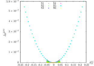
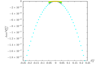
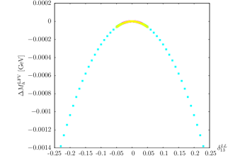
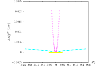
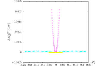
Figure 3: EWPO and Higgs masses as a function of slepton mixing $\delta^{LL}_{13}$ for the six points defined in the Tab. 1.

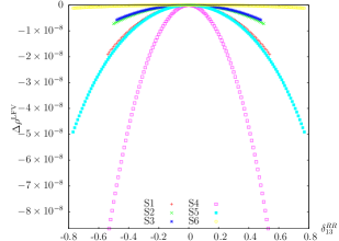
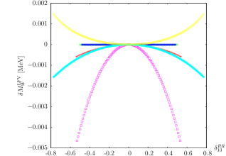
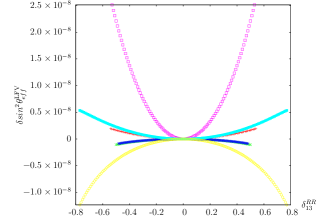
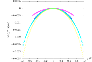
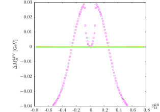
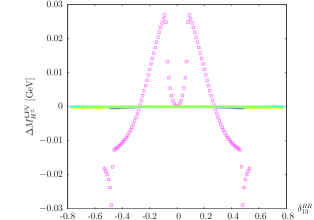
Figure 9: EWPO and Higgs masses as a function of slepton mixing $\delta^{RR}_{13}$ for the six points defined in the Tab. 1.

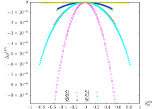
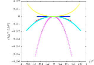
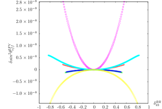
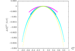
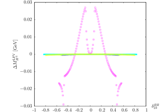
Figure 10: EWPO and Higgs masses as a function of slepton mixing $\delta^{RR}_{23}$ for the six points defined in the Tab. 1.

Our numerical results are shown in Figs. 3–10. The six plots in each figure are ordered as follows. Upper left: $\Delta\rho^{\text{LFV}}$, upper right: $\delta M_{W}^{\text{LFV}}$, middle left: $\delta\sin^{2}\theta_{\mathrm{eff}}^{\text{LFV}}$, middle right: $\Delta M_{h}^{\text{LFV}}$, lower left: $\Delta M_{H}^{\text{LFV}}$, and lower right: $\Delta M_{H^{\pm}}^{\text{LFV}}$, as a function of $\delta^{LL}_{13}$ (Fig. 3), $\delta^{LL}_{23}$ (Fig. 4), $\delta^{LR}_{13}$ (Fig. 5), $\delta^{LR}_{23}$ (Fig. 6), $\delta^{RL}_{13}$ (Fig. 7), $\delta^{RL}_{23}$ (Fig. 8), $\delta^{RR}_{13}$ (Fig. 9) and $\delta^{RR}_{23}$ (Fig.10). The legends are shown only in the first plot of each figure. We do not show results for LFV effects involving only the first and second generation. While they are included for completeness in our analytical results, they are expected to have a negligible effect on the observables considered here. The latter is confirmed by the numerical analysis presented in the next subsections.

4.1 EWPO

We start with the investigation of the LFV effects on the electroweak precision observables. Experimental bounds on the $\delta^{AB}_{12}$ are very strict (see Tab. 2) and hence it does not contribute sizably. The bounds on the other $\delta^{AB}_{ij}$’s are less strict but in most cases we still do not get appreciable contributions to the EWPO (but now can quantify their corresponding sizes). The only significant contribution comes from $\delta^{LL}_{23}$. The upper left plot in Fig. 4 shows our results for $\Delta\rho$ as functions of $\delta^{LL}_{23}$ under the presently allowed experimental range given in Tab. 2. Depending on the choice of scenario (S1…S6), values of ${\cal O}(10^{-3})$ can be reached. The largest values are found in S5, where the values of $\delta^{LL}_{23}$ of up to $\pm 0.3$ are permitted. For the same value of $\delta^{LL}_{23}$ we find the largest contributions in S6, which possesses the relatively largest values of soft-SUSY-breaking parameters in the slepton sector. This indicates that in general large contributions to the EWPO are possible as soon as heavy sleptons are involved. Conversely, while such heavy sleptons are in general difficult to detect directly at the LHC or the ILC, their presence could be visible in case of large LFV contributions via a shift in the EWPO.

Turning to the (pseudo-)observables $M_{W}$ and $\sin^{2}\theta_{\mathrm{eff}}$, respectively shown in the upper right and middle left plot of Fig. 4, we can compare the size of the LFV contributions to the current and future anticipated accuracies in these observables. The black line in both plots indicates the result for $\delta^{LL}_{23}=0$. The red line shows the current level of accuracy, Eq. (35), while the blue line indicates the future ILC/GigaZ precision, Eq. (36). We refrain from putting the absolute values of these observables since their values strongly depend on the choice of the stop/sbottom sector (see Ref. [6] and references therein), which is independent on the slepton sector under investigation here. While the current level of accuracy only has the potential to restrict $\delta^{LL}_{23}$ in S5 and S6, the future accuracy (particularly in $\sin^{2}\theta_{\mathrm{eff}}$) can set stringent bounds in all six scenarios.

The overall conclusion for the EWPO is that, while $\delta^{LL}_{23}$ is the most difficult one to restrict using ‘conventional’ LFV observables (see Sect. 3.2), it has (by far) the strongest impact on EWPO. Depending on the stop/sbottom sector, new bounds beyond the ‘conventional’ LFV observables can be obtained even with the current precision, and still better with the (anticipated) future accuracies.

4.2 Higgs masses

We now turn to the effects of the LFV contribtions on the prediction of the neutral ${\cal CP}$-even and the charged MSSM Higgs-boson masses. As discussed in Sect. 2.3, the theoretical accuracy should reach a precision of $\sim 50\,\,\mathrm{MeV}$ in the case of $M_{h}$ and about $\sim 1\%$ in the case of the heavy Higgs bosons. The calculation of $M_{h}$ in the presence of non-minimal flavor violation (NMFV) in the squark sector [5] indicated that corrections as large as ${\cal O}(10\,\,\mathrm{GeV})$ are possible (for the NMFV $\delta^{AB}_{ij}$ in agreement with all other precision data). Similar or even larger corrections were found for the heavy Higgs bosons, in particular for the charged Higgs boson. Large corrections were associated especially with non-zero values of $\delta^{LR,RL}_{23}$.

Even though the corrections from the slepton sector are naturally much smaller than from the squark sector, the LFV contributions could be expected to exceed future and possibly even current experimental uncertainties. Indeed, the estimated theoretical uncertainties for the LFV contributions of at least ${\cal O}(100\,\,\mathrm{MeV})$ for $M_{h}$ and ${\cal O}(10\,\,\mathrm{GeV})$ for $M_{H^{\pm}}$ were at the level of or exceeding the future anticipated accuracies. Thus, the LFV had to be evaluated and analyzed in order to reach the required level of precision.

The Higgs-boson masses are shown in the middle right plot ($M_{h}$), the lower left ($M_{H}$) and the lower right plot ($M_{H^{\pm}}$) of each figure. As expected from the NMFV analysis in the squark sector [5], the largest effects are found for $\delta^{LR,RL}_{23}$, but similarly for $\delta^{LR,RL}_{13}$, indicating that only the electroweak, not the Yukawa couplings, play a relevant role in these corrections. Contrary to expectations, the corrections to $M_{h}$ always stay below the level of a few MeV. Though this result obviates the above-mentioned uncertainty of ${\cal O}(100\,\,\mathrm{MeV})$, these contributions are too small to yield a sizable numerical effect.

Turning to the heavy Higgs bosons, the contributions to $M_{H}$ (most sizable again for $\delta^{LR,RL}_{23,13}$) do not exceed ${\cal O}(100\,\,\mathrm{MeV})$ and are thus effectively negligible. Substantially larger corrections are found, in agreement with the expectations from Ref. [5] for the charged Higgs-boson mass. They can reach the level of nearly $-2\,\,\mathrm{GeV}$, see Figs. 5–8. For the chosen values of $M_{A}$ (or $M_{H^{\pm}}$) this stays below the level of 1%. The absolute size of the corrections is not connected to the value of $M_{H^{\pm}}$ in S1…S6, however. Choosing starting values of $M_{A}$ somewhat smaller (requiring a new evaluation of the corresponding bounds on the LFV $\delta^{AB}_{ij}$), could yield relative corrections to $M_{H^{\pm}}$ at the level of 1%. Furthermore, as in the case of the light Higgs-boson mass, the explicit calculation of the LFV effects eliminates the theory uncertainty associated to these effects, thus improving the theoretical accuracy.

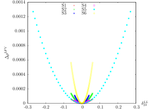
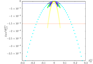
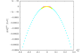
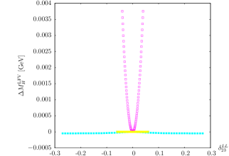
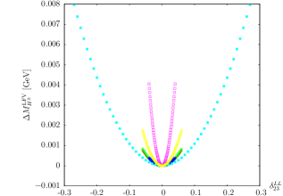
Figure 4: EWPO and Higgs masses as a function of slepton mixing $\delta^{LL}_{23}$ for the six points defined in the Tab. 1. Solid red (blue) line shows the present (future) experimental uncertainty.

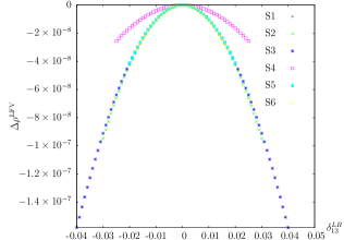
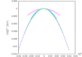
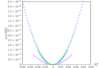
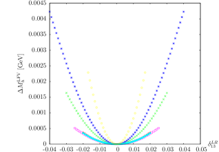
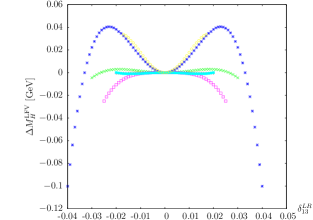
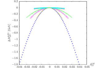
Figure 5: EWPO and Higgs masses as a function of slepton mixing $\delta^{LR}_{13}$ for the six points defined in the Tab. 1.

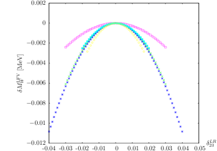
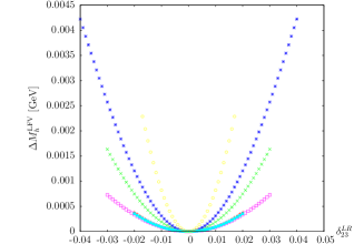
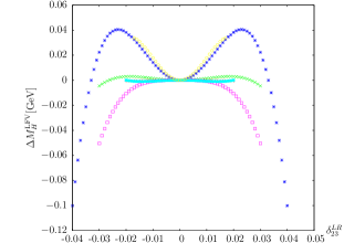
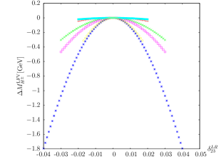
Figure 6: EWPO and Higgs masses as a function of slepton mixing $\delta^{LR}_{23}$ for the six points defined in the Tab. 1.

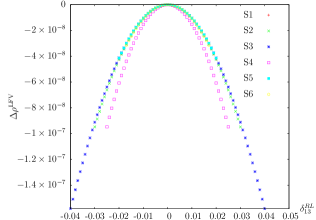
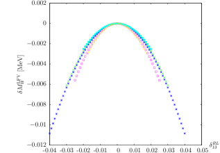
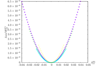
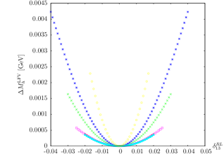
Figure 7: EWPO and Higgs masses as a function of slepton mixing $\delta^{RL}_{13}$ for the six points defined in the Tab. 1.

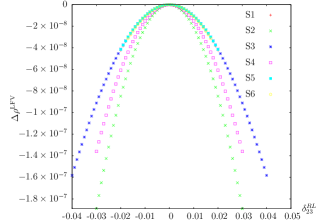
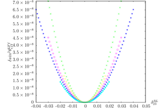
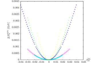
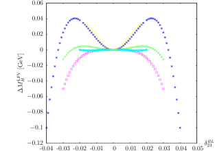
Figure 8: EWPO and Higgs masses as a function of slepton mixing $\delta^{RL}_{23}$ for the six points defined in the Tab. 1.

5 Conclusions

We extended Lepton Flavor Violation in the MSSM into the setup of FeynArts and FormCalc; the corresponding model file is part of the latest release of these programs.

The LFV effects are parameterized in a complete set of $\delta^{AB}_{ij}$ ($A,B=L,R$; $i,j=1,2,3$) without any assumption on the physics at the GUT scale. The inclusion of LFV into FeynArts/FormCalc allowed us to calculate the one-loop LFV effects on electroweak precision observables (via the calculation of gauge-boson self-energies) as well on the Higgs-boson masses of the MSSM (via the calculation of the Higgs-boson self-energies). The corresponding results have been included in the code FeynHiggs and are publicly available from version 2.10.2 on.

The numerical analysis was performed on the basis of six benchmark points defined in Ref. [20]. These benchmark points represent different combinations of parameters in the sfermion sector. The restrictions on the various $\delta^{AB}_{ij}$ in these six scenarios, provided by experimental limits on LFV processes (such as $\mu\to e\gamma$) have been taken from Ref. [20], and the effects on EWPO and Higgs-boson masses have been evaluated in the experimentally allowed ranges. In this way we provide a general overview about the possible size of LFV effects and potential new restrictions on the $\delta^{AB}_{ij}$ from EWPO and Higgs-boson masses.

The LFV effects in the EWPO turned out to be sizable for $\delta^{LL}_{23}$ but (at least in the scenarios under investigation) negligible for the other $\delta^{AB}_{ij}$. The effects of varying $\delta^{LL}_{23}$ in the experimentally allowed ranges turned out to exceed the current experimental uncertainties of $M_{W}$ and $\sin^{2}\theta_{\mathrm{eff}}$ in the case of heavy sleptons. No new general bounds could be set on $\delta^{LL}_{23}$, however, since the absolute values of $M_{W}$ and $\sin^{2}\theta_{\mathrm{eff}}$ strongly depend on the choices in the stop/sbottom sector, which is disconnected from the slepton sector presently under investigation. Such bounds could be set on a point-by-point basis in the LFV MSSM parameter space, however. Looking at the future anticipated accuracies, also lighter sleptons yielded contributions exceeding that precision. It may therefore be possible in the future to set bounds on $\delta^{LL}_{23}$ from EWPO that are stronger than from direct LFV processes.

In the Higgs sector, based on evaluations for flavor violation in the squark sector, non-negligible corrections to the light ${\cal CP}$-even Higgs mass as well as to the charged Higgs-boson mass could be expected. The associated theoretical uncertainties exceeded the anticipated future precision for $M_{h}$ and $M_{H^{\pm}}$. Taking the existing limits on the $\delta^{AB}_{ij}$ from LFV processes into account, however, the corrections mostly turned out to be small. For the light ${\cal CP}$-even Higgs mass they stay at the few-MeV level. For the charged Higgs mass they can reach ${\cal O}(2\,\,\mathrm{GeV})$, which, depending on the choice of the heavy Higgs-boson mass scale, could be at the level of the future experimental precision. More importantly, the theoretical uncertainty from LFV effects that previously existed for the evaluation of the MSSM Higgs-boson masses, has been reduced below the level of future experimental accuracy.

Acknowledgments

We thank M. Arana-Catania and M.J. Herrero for helpful discussions. The work of S.H. was partially supported by CICYT (grant FPA 2010–22163-C02-01). S.H. and M.R. were supported by the Spanish MICINN’s Consolider-Ingenio 2010 Programme under grant MultiDark CSD2009-00064.

References

• [1] Y. Kuno and Y. Okada, Rev. Mod. Phys. 73 (2001) 151 [arXiv:hep-ph/9909265].
• [2] H. Nilles, Phys. Rept. 110 (1984) 1;
H. Haber and G. Kane, Phys. Rept. 117 (1985) 75;
R. Barbieri, Riv. Nuovo Cim. 11 (1988) 1.
• [3] L. Hall, V. Kostelecky amd S. Raby, Nucl. Phys. B 267, 415 (1986).
• [4] F. Borzumati and A. Masiero, Phys. Rev. Lett. 57 (1986) 961.
• [5] M. Arana-Catania, S. Heinemeyer, M. Herrero and S. Penaranda, JHEP 1205 (2012) 015 [arXiv:1109.6232 [hep-ph]]; arXiv:1201.6345 [hep-ph]; arXiv:1405.6960 [hep-ph].
• [6] S. Heinemeyer, W. Hollik and G. Weiglein, Phys. Rept. 425 (2006) 265. hep-ph/0412214.
• [7] S. Heinemeyer, W. Hollik, F. Merz, S. Peñaranda, Eur. Phys. J. C 37 (2004) 481, hep-ph/0403228.
• [8] ATLAS Collaboration, ATLAS-CONF-2013-014, ATLAS-CONF-2013-025.
• [9] CMS Collaboration, CMS-PAS-HIG-13-005.
• [10] H. Baer et al., arXiv:1306.6352 [hep-ph].
• [11] J. Küblbeck, M. Böhm and A. Denner, Comput. Phys. Commun. 60 (1990) 165;
T. Hahn, Comput. Phys. Commun. 140 (2001) 418 [arXiv:hep-ph/0012260].
• [12] T. Hahn and C. Schappacher, Comput. Phys. Commun. 143 (2002) 54 [arXiv:hep-ph/0105349].
The program and the user’s guide are available via www.feynarts.de .
• [13] T. Fritzsche, T. Hahn, S. Heinemeyer, F. von der Pahlen, H. Rzehak and C. Schappacher, to appear in Comput. Phys. Commun., arXiv:1309.1692 [hep-ph].
• [14] T. Hahn and M. Pérez-Victoria, Comput. Phys. Commun. 118 (1999) 153 [arXiv:hep-ph/9807565].
• [15] S. Heinemeyer, W. Hollik and G. Weiglein, Comput. Phys. Commun. 124 (2000) 76 [arXiv:hep-ph/9812320];
T. Hahn, S. Heinemeyer, W. Hollik, H. Rzehak and G. Weiglein, Comput. Phys. Commun. 180 (2009) 1426; see www.feynhiggs.de .
• [16] S. Heinemeyer, W. Hollik and G. Weiglein, Eur. Phys. J. C 9 (1999) 343 [arXiv:hep-ph/9812472].
• [17] G. Degrassi, S. Heinemeyer, W. Hollik, P. Slavich and G. Weiglein, Eur. Phys. J. C 28 (2003) 133 [arXiv:hep-ph/0212020].
• [18] M. Frank, T. Hahn, S. Heinemeyer, W. Hollik, R. Rzehak and G. Weiglein, JHEP 0702 (2007) 047 [arXiv:hep-ph/0611326].
• [19] T. Hahn, S. Heinemeyer, W. Hollik, H. Rzehak and G. Weiglein, to appear in Phys. Rev. Lett., arXiv:1312.4937 [hep-ph].
• [20] M. Arana-Catania, S. Heinemeyer and M. Herrero, Phys. Rev. D 88 (2013) 015026 [arXiv:1304.2783 [hep-ph]].
• [21] S. Bilenky, S. Petcov and B. Pontecorvo, Phys. Lett. B 67 (1977) 309;
W. Marciano and A. Sanda, Phys. Lett. B 67 (1977) 303.
• [22] T. Cheng, L.-F. Li, Phys. Rev. Lett. 45 (1980) 1908.
• [23] A. Crivellin, L. Hofer and J. Rosiek, JHEP 1107 (2011) 017 [arXiv:1103.4272 [hep-ph]].
• [24] S. Heinemeyer, W. Hollik, H. Rzehak and G. Weiglein, Phys. Lett. B 652 (2007) 300 [arXiv:0705.0746 [hep-ph]].
• [25] J. Gunion, H. Haber, G. Kane and S. Dawson, The Higgs Hunter’s Guide, Addison-Wesley, 1990.
• [26] A. Dabelstein, Nucl. Phys. B 456 (1995) 25 [arXiv:hep-ph/9503443]; Z. Phys. C 67 (1995) 495 [arXiv:hep-ph/9409375].
• [27] A. Brignole, Phys. Lett. B 281 (1992) 284;
P. Chankowski, S. Pokorski and J. Rosiek, Phys. Lett. B 286 (1992) 307.
• [28] S. Gennai et al. Eur. Phys. J. C 52 (2007) 383 [arXiv:0704.0619 [hep-ph]].
• [29] The LEP Collaborations, the LEP Electroweak Working Group, the Tevatron Electroweak Working Group, the SLD Electroweak and Heavy Flavour Working Groups, Precision electroweak measurements and constraints on the Standard Model, CERN-PH-EP/2009-023; see http://www.cern.ch/LEPEWWG .
• [30] M. Baak et al., [arXiv:1310.6708[hep-ph]].
• [31] M. Veltman, Nucl. Phys. B 123 (1977) 89.
• [32] H. Haber and Y. Nir, Nucl. Phys. B 335 (1990) 363.
• [33] S. Chatrchyan et al. [CMS Collaboration], arXiv:1303.4571 [hep-ex];
Pedrame Bargassa, talk given at “Rencontres de Moriond EW 2014”,
https://indico.in2p3.fr/getFile.py/access?contribId=189&sessionId=0
&resId=1&materialId=slides&confId=9116
;
Mike Flowerdew, talk given at “Rencontres de Moriond EW 2014”,
https://indico.in2p3.fr/getFile.py/access?contribId=169&sessionId=0
&resId=0&materialId=slides&confId=9116
;
Paul Thompson, talk given at “Rencontres de Moriond EW 2014”,
https://indico.in2p3.fr/getFile.py/access?contribId=220&sessionId=8
&resId=0&materialId=slides&confId=9116
;
Kevin Einsweiler, talk given at “Rencontres de Moriond EW 2014”,
https://indico.in2p3.fr/getFile.py/access?contribId=227&sessionId=1
&resId=1&materialId=slides&confId=9116
.
• [34] P. Bechtle, O. Brein, S. Heinemeyer, G. Weiglein and K. Williams, Comput. Phys. Commun. 181 (2010) 138 [arXiv:0811.4169 [hep-ph]]; Comput. Phys. Commun. 182 (2011) 2605 [arXiv:1102.1898 [hep-ph]];
P. Bechtle, O. Brein, S. Heinemeyer, O. Stål, T. Stefaniak, G. Weiglein and K. Williams, Eur. Phys. J. C 74 (2014) 2693 [arXiv:1311.0055 [hep-ph]].
• [35] M. Awramik, M. Czakon, A. Freitas and G. Weiglein, Phys. Rev. D 69 (2004) 053006 [arXiv:hep-ph/0311148].
• [36] M. Awramik, M. Czakon, A. Freitas and G. Weiglein, Phys. Rev. Lett. 93 (2004) 201805 [arXiv:hep-ph/0407317].
• [37] T. Hahn, W. Hollik, J.I. Illana, S. Peñaranda, arXiv:hep-ph/0512315.