Dynamical preparation of laser-excited anisotropic Rydberg crystals in 2D optical lattices

Abstract

We describe the dynamical preparation of anisotropic crystalline phases obtained by laser-exciting ultracold Alkali atoms to Rydberg p-states where they interact via anisotropic van der Waals interactions. We develop a time-dependent variational mean field ansatz to model large, but finite two-dimensional systems in experimentally accessible parameter regimes, and we present numerical simulations to illustrate the dynamical formation of anisotropic Rydberg crystals.

Keywords: Rydberg atoms, Driven Rydberg gas, Anisotropic interactions, Dynamical crystallization, Dynamical state preparation

1 Introduction

Highly excited Rydberg states of atoms have unique properties. This includes the size of the Rydberg orbitals scaling as $n^{2}$, the polarizabilities as $n^{7}$ and a long lifetime as $n^{3}$ with $n$ the principal quantum number. These properties are also manifest in interactions between Rydberg states, e.g. in van der Waals (vdW) interactions $\propto n^{11}/r^{6}$, which can be controlled and tuned via external fields. Exciting ground state atoms with a laser to Rydberg states thus provides a means to study many body systems with strong, long-range interactions [1, 2]. With the atomic ground state and the Rydberg state defining an effective spin-$1/2$, we can describe the many body dynamics in terms of a model of interacting spins [3, 4, 5], reflecting the competition between the laser excitation and vdW interactions, at least in the short time limit where the motion of the atoms can be neglected (the so-called frozen gas regime).

The study of quantum phases of a laser excited Rydberg gas of alkali atoms, including its dynamical preparation, has so far focused on isotropic vdW interactions, corresponding to Rydberg s-states excited in a two-photon process. This includes theoretical studies [6, 7, 8, 9, 10, 11] and experimental observations [12, 13] of Rydberg crystals due to the Rydberg blockade mechanism [14, 15, 16, 17, 18, 19, 20], and their melting with increasing laser intensity to a quantum-disordered phase [21, 22]. The steady state of the system has also been studied in presence of dissipation [23, 24, 25, 26]. With the availability of UV laser sources also Rydberg p-states can be excited in a single photon transition, leading to anisotropic vdW interactions [27, 28]. The goal of this paper is to investigate the quantum phases and their dynamical preparation with a laser pulse protocol for these anisotropic interactions. We are interested in 2D systems with a relatively high density of excitations involving a larger number of atoms, and in particular in the dynamical formation of anisotropic Rydberg crystals. Our studies are performed within a time-dependent variational mean field ansatz, beyond what can be accessed by exact diagonalization techniques.

2 Model and Method

2.1 Laser excited interacting Rydberg atoms as an anisotropic spin model

We are interested in the quantum dynamics and the quantum phases of a gas of laser excited Rydberg atoms, interacting via anisotropic vdW interactions. The setup we have in mind is represented in figure 1. We assume that the atoms are trapped in a 2D square lattice with exactly one atom per lattice site, as obtained in a Mott insulator phase. The atoms are initially prepared in the ground state, denoted by $\mid\downarrow\rangle$, and coherently excited by a laser to a Rydberg state $\mid\uparrow\rangle$ with Rabi frequency $\Omega$ and laser detuning $\Delta$ [see figure 1(a)]. Two atoms $i$ and $k$ both excited to the Rydberg state $\mid\uparrow\rangle$ and located at positions $\mathbf{r}_{i}$ and $\mathbf{r}_{k}$, respectively, interact via vdW interactions $V(\mathbf{r}_{i}-\mathbf{r}_{k})=C_{6}(\theta_{i,k})/|\mathbf{r}_{i}-\mathbf{r}_{k}|^{6}$. These vdW interactions exceed typical ground state interactions of cold atoms by several orders of magnitude. We are interested in a situation where the vdW interaction has a non-trivial angular dependence $C_{6}(\theta_{i,k})$. Such an angular dependence arises, for example, in laser excitation to higher angular momentum states, e.g. to Rydberg $p$-states, as opposed to excitation of $s$-states where the interactions are isotropic [27]. In the remainder of this paper we will illustrate the anisotropic interactions by explicitly considering the stretched state $|n^{2}P_{3/2},m_{j}=3/2\rangle$ of Rubidium for which the $C_{6}(\theta_{i,k})$ is dominated by a term proportional to $\sin^{4}\theta_{i,k}$ [28]. Interactions are therefore much stronger along the $x$ direction compared to the $z$ direction [see figure 1(b)]. The atomic physics underlying this interaction will be discussed in detail in section 3 below.

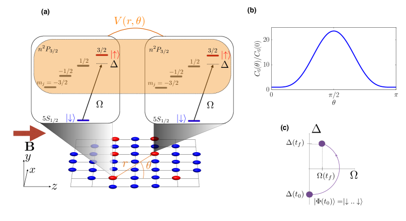
Figure 1: (a) Setup: The ground state atoms $\mid\downarrow\rangle$ are placed in a square optical lattice and are excited to a Rydberg state $\mid\uparrow\rangle$ via a homogeneous laser beam with Rabi frequency $\Omega$ and detuning $\Delta$. The vdW interaction $V$ between two Rydberg atoms $i$ and $k$ is a function of their relative distance $|\mathbf{r}_{i}-\mathbf{r}_{k}|$ but also of the angle $\theta_{i,k}$ between their relative vector and the magnetic field $B$ which is set along the $z$ direction of the lattice. The details of these interactions in the fine structure manifold $n^{2}P_{3/2}$, in the presence of the magnetic field are discussed in section 3. (b) Example of angular dependence of the $C_{6}$ coefficient obtained for a Rydberg state of Rubidium $|25P_{3/2},m_{j}=3/2\rangle$. (c) Example of sweep path: initially the atoms are prepared in the ground state $\mid\downarrow\rangle$ with a negative detuning $\Delta(t_{0})<0$. The Rabi frequency $\Omega$ and the laser detuning $\Delta$ are then slowly varied to reach the final state of the preparation at time $t_{f}$.

In its simplest form the dynamics of the driven Rydberg gas can be described by an interacting system of pseudospin-1/2 particles

$${H}=\frac{\hbar}{2}\sum_{i=1}^{N}\left(\Omega\sigma^{(i)}_{x}-\Delta\sigma^{(i)}_{z}\right)+\frac{1}{2}\sum_{i=1}^{N}\sum_{\substack{k=1,k\neq i}}^{N}\frac{C_{6}(\theta_{i,k})P_{i}P_{k}}{\mid\mathbf{r}_{i}-\mathbf{r}_{k}\mid^{6}}$$ (1)

where $\sigma^{(i)}_{x}=\mid\uparrow\rangle_{i}\langle\downarrow\mid+\mid\downarrow\rangle_{i}\langle\uparrow\mid$ and $\sigma^{(i)}_{z}=\mid\uparrow\rangle_{i}\langle\uparrow\mid-\mid\downarrow\rangle_{i}\langle\downarrow\mid$ correspond to the local Pauli matrices and $P_{i}=\mid\uparrow\rangle_{i}\langle\uparrow\mid$ is the projection operator on the Rydberg level. We note that in this model atoms are assumed to be pinned to the lattice sites, which is referred to as the frozen gas approximation [2]. For isotropic interactions spin models of this type have been discussed in previous theoretical work [6, 7, 9, 8, 10, 11], and have been the basis for interpreting experiments [12, 13].

The modeling of the laser excited Rydberg gas as a coherent spin dynamics governed by the Hamiltonian (1) is valid for sufficiently short times. First, as we noted above, the model (1) ignores the motion of the atoms: laser excited Rydberg atoms are typically not trapped by the optical lattice for the ground state atoms, and there will be (large) mechanical forces associated with the vdW interactions. In addition, Rydberg states have a finite life time, scaling as $\tau\sim n^{3}$ $(\tau\sim n^{5})$ for low (high) angular momentum states with $n$ the principal quantum number, and black body radiation can drive transitions between different Rydberg states, further decreasing the lifetime by approximately a factor of two [29]. The regime of validity has been analyzed in detail in [30]: there the long time dynamics of laser excited Rydberg gas including motion and dissipation was treated, including the validity of the frozen gas approximation and the cross over regime.

We emphasize that the various quantum phases predicted by the spin model (1) as a function of the laser parameters and interactions, and their preparation in an experiment, can only be understood in a dynamical way. In an experiment all atoms are initially prepared in their atomic ground state, $|\Phi(t_{0})\rangle=|G\rangle\equiv\mid\downarrow\rangle_{1}\ldots\mid\downarrow\rangle_{N}$, which is the ground state of the many-body Hamiltonian (1) for $\Omega=0$ and $\Delta<0$. Preparation of the ground state of the spin Hamiltonian (1) for a given $\Omega$ and $\Delta$ can thus be understood in the sense of adiabatic state preparation, where starting from an initial time $t_{0}$ with laser parameters $\Omega(t_{0})=0$ and $\Delta(t_{0})<0$ we follow the evolution of the many body state for a parameter trajectory to the final time $t_{f}$ with $\Omega(t_{f})=\Omega$ and $\Delta(t_{f})=\Delta$, see figure 1(c). This dynamical preparation of many-body states and quantum phases of the spin-model (1) in a time-dependent mean field ansatz, in particular in the anisotropic case, will be a central question to be addressed below.

While our focus below will be on the anisotropic model, we find it worthwhile to summarize the basic properties and signatures of the quantum phases (ground states) of the spin model (1) for isotropic interactions. Even for this case, the ground-state phase diagram of the Hamiltonian (1) is rather complicated. In the so-called classical limit, $\Omega\rightarrow 0$, where all terms in the Hamiltonian (1) commute, the ground-state corresponds to the minimum energy configuration of classical charges on a square lattice interacting via a $1/r^{6}$ potential, and $\Delta$ serves as a chemical potential [31]. As noted above, for $\Delta<0$ this corresponds to the state $|G\rangle$ with all atoms in the ground state. For $\Delta>0$ a finite density of excited Rydberg atoms is energetically favorable and the competition between the laser detuning and the vdW interactions results in a complex crystalline arrangement with a typical distance between excited atoms set by the length scale $\ell\equiv[C_{6}/(\hbar\Delta)]^{1/6}$. In two dimensions the Rydberg atoms ideally want to form a triangular lattice to maximize their distance, which will compete with the square optical lattice for the setup of figure 1. An exact solution of this classical commensurability problem is not known except in one dimension, where all possible commensurate crystalline phases form a complete devil’s staircase [32]. In analogy to the 1D case we expect a plethora of different crystalline phases in two dimensions, which are stable over some part of the phase diagram and which break the lattice symmetries in different ways [33, 34, 31].

Away from the classical limit, $\Omega\neq 0$, the crystalline states of Rydberg atoms are expected to be stable for sufficiently small $\Omega$. By increasing $\Omega$ quantum fluctuations will eventually melt the crystalline phases and we reach a quantum disordered phase. The nature of the corresponding quantum phase-transition has been studied in one dimension [21, 22] and remains an open issue in higher dimensions.

Concerning anisotropic interactions, it is natural to expect that the angular dependence of the vdW coefficient, $C_{6}(\theta_{i,k})$, is responsible for the presence of an anisotropic crystalline phase at small $\Omega$. In summary, our goal below is to describe the dynamical formation of such crystals in large but finite systems similar to realistic experimental situations, where finite size effects still play an important role, and to compare the final state to the ground state of the system in order to assess the fidelity of the dynamical preparation. To this end, we developed an approach based on a time-dependent variational principle which proved very useful to describe the crystalline states for isotropic as well as anisotropic interactions with a large number of excitations, i.e. in a parameter regime where an exact solution cannot be applied.

2.2 Time dependent variational ansatz for many-body systems

In the following we present our variational ansatz and the corresponding equations of motion which we use to describe the dynamical preparation of Rydberg crystals governed by (1). The simplest variational ansatz which is able to describe crystalline states of Rydberg atoms takes the most general product state form

$$|\Phi(t)\rangle = \bigotimes_{i=1}^{N}\left[\alpha_{i}(t)\mid\downarrow\rangle_{i}+\beta_{i}(t)\mid\uparrow\rangle_{i}\right],$$ (2)

where $N$ denotes the number of atoms and the coefficients $\alpha_{i}$ and $\beta_{i}$ obey the normalization condition $|\alpha_{i}|^{2}+|\beta_{i}|^{2}=1$. Crystalline phases correspond to states where the probability $|\beta_{i}|^{2}$ to find an atom in the Rydberg state at lattice site $i$ is spatially modulated and its Fourier components serve as an infinite set of order parameters. In contrast, in the quantum disordered phase the Rydberg density is homogeneous and $|\beta_{i}|^{2}$ is equal on all lattice sites $i$.

2.2.1 Equilibrium properties of the variational ansatz

Before deriving equations of motion for the time dependent variational parameters $\alpha_{i}(t)$ and $\beta_{i}(t)$ we discuss equilibrium properties of our variational ansatz. Note that the ansatz (2) captures the exact ground- and excited states of our model Hamiltonian [equation (1)] in the classical limit $\Omega\to 0$, where all eigenstates are product states. In the general case $\Omega>0$, it is an approximation and its validity will be discussed at the end of this subsection. In principle we find the variational ground-state by minimizing the expectation value of the Hamiltonian with respect to the variational parameters $\alpha_{i}$ and $\beta_{i}$. In the ground-state these parameters can be chosen to be real and the variational ground-state energy, $E=\langle\Phi|H|\Phi\rangle$, can be expressed as function of the probabilities $p_{i}=|\beta_{i}|^{2}$ as

$$E(p_{i}) = -\hbar\Omega\sum_{i}\sqrt{p_{i}(1-p_{i})}-\hbar\Delta\sum_{i}(p_{i}-\frac{1}{2})$$ (3)

$$+\frac{1}{2}\sum_{k\neq i}V(\mathbf{r}_{i}-\mathbf{r}_{k})p_{i}p_{k}$$

with $V(\mathbf{r}_{i}-\mathbf{r}_{k})=C_{6}(\theta_{i,k})/|\mathbf{r}_{i}-\mathbf{r}_{k}|^{6}$. Finding all solutions of the corresponding mean-field equations $\partial E(p_{i})/\partial p_{i}=0$ in the thermodynamic limit is an impossible task, however. For this reason we do not attempt to make predictions about the phase diagram of (1) in the thermodynamic limit and rather focus on experimentally relevant systems with a finite but large number of atoms instead.

There is one notable exception, however: we can make a statement about the melting transition between the quantum disordered phase at large $\Omega$ and the adjacent crystalline phase within our variational (mean-field) approach. In the thermodynamic limit, the quantum disordered phase has a homogeneous Rydberg density $f_{R}:=p_{i}\equiv p$ and we can determine at which point the homogeneous solution becomes unstable to density modulations. Linearizing the mean-field equations in small perturbations around the homogeneous solution we find the condition

$$1+\frac{\hbar^{2}\Omega^{2}}{\big{[}(V_{0}f_{R}-\hbar\Delta)^{2}+\hbar^{2}\Omega^{2})\big{]}^{3/2}}\ \min_{\mathbf{k}}(V_{\mathbf{k}})=0\ ,$$ (4)

where $V_{\mathbf{k}}=\sum_{i}e^{{\mathrm{i}}\mathbf{k}\cdot\mathbf{R}_{i}}V(\mathbf{R}_{i})$ are Fourier components of the interaction potential (note that the density $f_{R}$ of Rydberg excitations depends on $\Omega$ and $\Delta$). We note that an expansion in small density modulations around the homogeneous solution implicitly assumes that the melting transition is continuous. It is possible that this transition could be first order, however. In order to rule out a discontinuous melting transition we minimized the variational energy (3) numerically on a lattice with $N=441$ sites and found that the melting transition is indeed continuous.

The momentum $\mathbf{k}_{0}$ at which the interaction potential $V_{\mathbf{k}}$ is minimal determines the wave-vector at which density modulations form in the crystalline phase. In the isotropic case this minimum is at $\mathbf{k}_{0}=(k_{0}^{x},k_{0}^{z})=(\pi/a,\pi/a)$, where $a$ is the lattice constant of the optical lattice. If one approaches the crystalline phase from the quantum disordered phase, the leading instability is thus always towards a crystalline state with Neel-type order, which breaks a $Z_{2}$ lattice symmetry. Only at smaller $\Omega$ more complicated crystalline states appear, which are most likely separated by first order phase transitions. Consequently, within our variational approach the quantum phase transition between the disordered and the crystalline phase is always in the Ising universality class for isotropic interactions, independent of $\Omega$ and $\Delta$.

For an anisotropic interaction potential with angular dependence $C_{6}(\theta_{i,k})$, present for example between $\mid\uparrow\rangle=|n^{2}P_{3/2},m_{j}=3/2\rangle$ states of Rubidium as discussed in section 3, the minimum is at a wave-vector $\mathbf{k}_{0}=(\pi/a,0)$. Again, if we approach the crystalline phase from the quantum-disordered regime, crystalline order will form only in $x$-direction with a period of two lattice spacings, whereas no crystalline order is present in $z$-direction. This transition is again continuous. The system thus decouples into an array of quasi one dimensional Rydberg gases. Upon further decreasing $\Omega$, we expect a transition to a state with incommensurate, floating crystalline order in $z$-direction, in analogy to one-dimensional systems [21, 22]. The system remains long-range ordered in $x$-direction, however, and finally settles into a commensurate, genuinely two-dimensional crystalline state at sufficiently small $\Omega$. We leave a detailed investigation of this two-step directional melting transition open for future study.

The phase boundary obtained from (4) is shown in figure 2 for both isotropic as well as anisotropic interactions with the angular dependence represented in figure 1(b). As in the anisotropic case the interactions are much stronger in the $x$ direction compared to the $z$-direction, the corresponding phase-boundary significantly differs from the isotropic curve and is very close to the one obtained for a one-dimensional system. Note that the mean-field phase boundary has an unphysical re-entrance behavior at negative detunings. This is because our variational ansatz vastly overestimates the ground-state energy in the quantum disordered phase at finite $\Omega$, where pair-correlations are important.

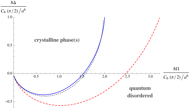
Figure 2: Mean-field phase boundary between the quantum-disordered and crystalline phase(s) obtained from (4). The blue solid line represents the case of anisotropic interactions with the angular dependence $C_{6}(\theta)$ of Rubidium $|nP_{3/2},m_{j}=3/2\rangle$ atoms [see figure 1(c)]. The red dashed line shows the phase boundary for isotropic interactions. For comparison, the black dotted line represents the mean-field phase boundary of a one-dimensional system.

Indeed, our product ansatz of (2) does not describe correlations between local density fluctuations of Rydberg atoms

$$\langle\delta P_{i}\delta P_{k}\rangle=\langle P_{i}P_{k}\rangle-\langle P_{i}\rangle\langle P_{k}\rangle\ ,$$ (5)

and thus $\langle\delta P_{i}\delta P_{k}\rangle_{\Phi}\equiv 0$ for our variational wave-function. Deep in the crystalline phase these correlations are weak and decay exponentially with distance, however. We can give an upper bound on the strength of such density density correlations and consequently make a statement about the validity of our ansatz by estimating the strength of local density fluctuations

$$\langle{\delta P_{i}}^{2}\rangle=\langle P_{i}\rangle(1-\langle P_{i}\rangle)\ .$$ (6)

Accordingly, density-density correlations are negligible deep in the crystal, where $\langle P_{i}\rangle$ is either close to zero or one. As a consequence we expect our ansatz to be valid also at finite $\Omega$ as long as we are deep in the crystalline phase. At sufficiently large $\Omega$, where the system enters the quantum disordered phase and quantum correlations become predominant, our ansatz is not a good approximation for the exact ground-state wave function.

2.2.2 Time-dependent variational ansatz and Euler-Lagrange equations

One of the main goals of our paper is to describe the dynamical formation of crystalline states of Rydberg excitations in a large but finite system during a slow change of the laser parameters. For this reason we incorporate our ansatz into a time-dependent variational approach, where the formation of Rydberg excitations is described by the time evolution of the variational coefficients $\alpha_{i}(t)$ and $\beta_{i}(t)$ and governed by the Hamiltonian (1). Considering an initial condition where all atoms are in the ground state $|G\rangle$, i.e. $\alpha_{i}(t_{0})=1\ (\forall i\in\{1,\dots,N\})$ and $\Omega(t_{0})=0$, $\Delta(t_{0})<0$, we use the time-dependent variational principle (TDVP) [35] to derive the equations of motion for the variational coefficients during a slow change of $\Omega$ and $\Delta$ as in typical dynamical state preparation schemes [8, 9, 13]. The TDVP states that the time-evolution of the variational coefficients satisfy the least action principle which means that they can be derived using the Euler-Lagrange equations:

$$\frac{d}{dt}\left(\frac{\partial L}{\partial\dot{\alpha}_{i}^{*}}\right) = \frac{\partial L}{\partial\alpha_{i}^{*}}$$

$$\frac{d}{dt}\left(\frac{\partial L}{\partial\dot{\beta}_{i}^{*}}\right) = \frac{\partial L}{\partial\beta_{i}^{*}}$$

where $L$ is the Lagrangian

$$L = \frac{{\mathrm{i}}\hbar}{2}\langle\Phi|d_{t}\Phi\rangle-\frac{{\mathrm{i}}\hbar}{2}\langle d_{t}\Phi|\Phi\rangle-\langle\Phi|H|\Phi\rangle.$$

leading to a set of $2N$ non-linear coupled equations

$${\mathrm{i}}\hbar\dot{\alpha_{i}} = \frac{\hbar\Omega}{2}\beta_{i}+\frac{\hbar\Delta}{2}\alpha_{i}$$

$${\mathrm{i}}\hbar\dot{\beta_{i}} = \frac{\hbar\Omega}{2}\alpha_{i}-\frac{\hbar\Delta}{2}\beta_{i}+\sum_{k\neq i}\frac{C_{6}(\theta_{i,k})}{|\mathbf{r}_{i}-\mathbf{r}_{k}|^{6}}|\beta_{k}|^{2}\beta_{i}.$$ (7)

We note that these equations conserve the norm of the wavefunction for all times, i.e. $|\alpha_{i}(t)|^{2}+|\beta_{i}(t)|^{2}=1$. If $\Omega$ and $\Delta$ do not evolve in time, the expectation value of the energy $E=\langle\Phi|H|\Phi\rangle$ is also a conserved quantity. However, this is not the case for a dynamical state preparation and the final energy depends crucially on the parameter trajectory.

In a perfectly adiabatic situation we would obtain the variational ground-state for $\Omega(t_{f})$ and $\Delta(t_{f})$ at the end of the time evolution. Since our sweep protocols are limited to timescales smaller than the lifetime of the Rydberg state, the preparation will not be perfectly adiabatic and we discuss deviations from adiabaticity in subsection 4.1. We note that given the phase diagram shown in figure 2 and the typical parameter sweep we consider [figure 1(b)], the system has to undergo a quantum phase transition from the quantum disordered phase to the crystalline phase at some point in the preparation which may reduce the adiabaticity of the preparation significantly. In the finite systems that we consider in the rest of this work, a finite-size gap is always present which reduces this problem, however.

Finally, we note that our ansatz (2) is particularly suited to study the experimentally relevant situation where the Rydberg laser is switched off at the end of the parameter sweep $\Omega(t_{f})=0$, because it captures the exact ground- and excited states of the Hamiltonian (1) in the classical limit $\Omega=0$, as discussed above. In subsection 4.1 we also estimate the typical Rabi frequency $\Omega$ at which our ansatz fails by comparing our approach to the exact solution of the Schrödinger equation.

In the next section, we explain in detail the implementation of the model Hamiltonian (1) with Rydberg atoms excited to $\mid\uparrow\rangle=|n^{2}P_{3/2},m_{j}=3/2\rangle$ Rydberg states in order to provide realistic parameters for our numerical section 4.

3 Anisotropic interactions for Rydberg atoms in p-states

In the following we discuss the derivation of our model Hamiltonian [equation (1)] from a microscopic Hamiltonian,

$$H_{\rm mic}=\sum_{i=1}^{N}\left[H_{A}^{(i)}+H_{L}^{(i)}\right]+\frac{1}{2}\sum_{i=1}^{N}\sum_{\substack{k=1,k\neq i}}^{N}H_{V}^{(i,k)}.$$ (8)

describing vdW interactions between $N$ alkali atoms laser excited to the $\mid\uparrow\rangle\equiv|nP_{3/2},m_{j}=3/2\rangle$ Rydberg state. We first focus on the Rydberg manifold and their interactions and then discuss the laser excitations. The first term of (8),

$$H_{A}^{(i)}=\sum_{m_{j}}\left[\hbar\omega_{nP_{3/2}}+\mu_{B}g_{j}B_{z}m_{j}\right]|m_{j}\rangle\langle m_{j}|,$$ (9)

accounts for the energies of the Zeeman sublevels $|m_{j}\rangle\equiv|nP_{3/2},m_{j}\rangle$ with $m_{j}\in\{-3/2,\ldots,3/2\}$ as illustrated in figure 1. Here, $\hbar\omega_{nP_{3/2}}$ is the energy difference between the atomic ground state, $5S_{1/2}$, and the $nP_{3/2}$ Rydberg manifold in the absence of external fields. The second term of $H_{A}^{(i)}$ describes the lifting of the energy degeneracy of the $nP_{3/2}$ Rydberg manifold due to a magnetic field $\mathbf{B}=B\mathbf{e}_{z}$ (see figure 1), with $\mu_{B}/h=1.4$ MHz/G the Bohr magneton and $g_{j}$ the Lande factor for $j=3/2$. Note, that the quantization axis of the corresponding eigenstates is given by the direction of the magnetic field, $\mathbf{B}$, and is aligned in plane along the $z$-axis, see figure 1. In order to neglect higher order shifts and to prevent mixing between different fine-structure manifolds the energy shifts $\Delta E_{m_{j}}=\mu_{B}g_{j}B_{z}m_{j}$ have to be much smaller than the fine-structure splitting $E_{nP_{3/2}}-E_{nP_{1/2}}$ of the Rydberg manifolds. Typically, the fine structure splitting is of the order of tens of GHz, e.g. 7.9 GHz for $n=25$.

Away from Foerster resonances two laser excited Rydberg atoms dominantly interact via van der Waals interactions [1, 2]. In general, these van der Waals interactions, $\hat{V}_{\rm vdW}$, will mix different Zeeman sublevels $|m_{j}\rangle$ in the $nP_{3/2}$ manifold [36]. Let us denote by $\hat{P}=\sum_{i,j}|m_{i},m_{j}\rangle\langle m_{i},m_{j}|$ a projection operator into the $nP_{3/2}$ manifold, then the dipole-dipole interactions $\hat{V}_{\rm dd}$ will couple to intermediate states, $\hat{Q}_{\alpha,\beta}=|\alpha,\beta\rangle\langle\alpha,\beta|$, which have an energy difference $\delta_{\alpha\beta}$. In second order perturbation this gives rise to

$$\hat{V}_{\rm vdW}=\hat{P}\sum_{\alpha\beta}\frac{\hat{V}_{\rm dd}\hat{Q}_{\alpha,\beta}\hat{V}_{\rm dd}}{\delta_{\alpha\beta}}\hat{P},$$ (10)

where $\hat{V}_{\rm vdW}$ is understood as an operator acting in the manifold of Zeeman sublevels We note, that in the absence of an external magnetic field, $\mathbf{B}\rightarrow 0$, the new eigenenergies obtained from diagonalizing $\hat{V}_{\rm vdW}$ are isotropic.

Anisotropic van der Waals interactions can be obtained by lifting the degeneracy between the Zeeman sublevels e.g. with a magnetic field. For distances large enough, such that the off-diagonal vdW coupling matrix elements of (10) are much smaller than the energy splitting between the Zeeman sublevels, it is possible to simply consider interactions between $|nP_{3/2},m_{j}=3/2\rangle$ states and neglect transitions to different $m_{j}$ levels. Typically, for Rydberg $p$-states the off-diagonal vdW matrix elements are of the same order as the diagonal interaction matrix elements. Pairwise interactions between two atoms excited to the $\mid\uparrow\rangle=|nP_{3/3},m_{j}=3/2\rangle$ state are then described by the Hamiltonian

$$H^{(i,k)}_{V}=V(\mathbf{r}_{i}-\mathbf{r}_{k})\mid\uparrow\rangle_{i}\langle\uparrow\mid\otimes\mid\uparrow\rangle_{k}\langle\uparrow\mid,$$ (11)

where $V(\mathbf{r}_{i}-\mathbf{r}_{k})=\langle{\textstyle\frac{3}{2},\frac{3}{2}}|\hat{V}_{\rm vdW}|{\textstyle\frac{3}{2},\frac{3}{2}}\rangle=C_{6}(\theta_{i,k})/|\mathbf{r}_{i}-\mathbf{r}_{k}|^{6}$ the van der Waals interaction potential, giving rise to the second term of (1). Here, $\theta_{i,k}=\sphericalangle(\mathbf{B},\mathbf{r}_{i}-\mathbf{r}_{k})$ is the angle between the relative vector and the quantization axis given by the magnetic field direction $\mathbf{B}$ (see figure 1).

The second term of (8), $H_{L}^{(i)}$, accounts for the laser excitation of Rubidium ⁸⁷Rb atoms prepared in their electronic ground state, which we choose as $\mid\downarrow\rangle=|5^{2}S_{1/2},F=2,m_{F}=2\rangle$, to the $\mid\uparrow\rangle=|nP_{3/2},m_{j}=3/2\rangle$ Rydberg states. This can be done using a single-photon transition with Rabi frequency $\Omega$, scaling as $\Omega\sim n^{-3/2}$. Using a UV laser source it is possible to obtain Rabi frequencies of several MHz in order to excite Rydberg states around $n\sim 30$. The single particle Hamiltonian governing the laser excitation of atom $i$ is

$$H_{L}^{(i)}(t)=\frac{\hbar\Omega}{2}\left(\mid\uparrow\rangle_{i}\langle\downarrow\mid e^{i(\mathbf{k}_{L}\cdot\mathbf{r_{i}}-\omega_{L}t)}+\mid\downarrow\rangle_{i}\langle\uparrow\mid e^{-i(\mathbf{k}_{L}\cdot\mathbf{r_{i}}-\omega_{L}t)}\right),$$ (12)

where $\omega_{L}=\omega_{nP_{3/2}}+\Delta E_{3/2}/\hbar+\Delta$ is the laser frequency detuned by $\Delta$ from the atomic transition (including the magnetic field splitting) and $\mathbf{k}_{L}$ is the wave vector of the laser. Unwanted couplings to Zeeman levels with $m_{j}\neq 3/2$ due to the laser can be prevented by using a detuning $|\Delta|\ll|\Delta E_{3/2}-\Delta E_{1/2}|$ or by using circular polarized light propagating along the quantization axis, i.e. $\mathbf{k_{L}}\sim\mathbf{\hat{z}}$, which couples $\mid\downarrow\rangle$ only to the $m_{j}=3/2$ state. In a frame rotating with the laser frequency and after absorbing the position dependent phase into $\mid\uparrow\rangle_{i}\rightarrow e^{-i\mathbf{k}_{L}\cdot\mathbf{r_{i}}}\mid\uparrow\rangle_{i}$ one obtains the first term of (1).

As an example, we consider the $n=25$ Rydberg state, i.e. $\mid\uparrow\rangle\equiv|25P_{3/2},m_{j}=\frac{3}{2}\rangle$. For the corresponding diagonal van der Waals matrix element we obtain using the model potential from [37]

$$C_{6}(\theta)=\left(6.33\sin^{4}\theta-0.267\sin^{2}\theta+0.269\right)h\,\mathrm{MHz}\,\mu\mathrm{m}^{6}.$$ (13)

Thus, $C_{6}(\pi/2)=6.35\,h\,\mathrm{MHz}\,\mu\mathrm{m}^{6}$ and $C_{6}(0)=0.269\,h\,\mathrm{MHz}\,\mu\mathrm{m}^{6}$. The dominant $\sim\sin^{4}\theta$ term arises from dipole-dipole transitions to $nS_{1/2}$ states, while residual interactions at $\theta=0$ and deviations from the $\sim\sin^{4}\theta$ shape originate from couplings to $D$-channels as discussed in [27]. The lifetime of the Rydberg state is $\tau\approx 29\ \mu$s [29].

We finally note that it is also possible to switch from the anisotropic configuration defined above to an isotropic configuration where the angle $\theta$ is fixed to a constant value $\frac{\pi}{2}$. In this configuration, the magnetic field is rotated from the $z$ to the $y$-direction (see figure 1) and the Rydberg state which is excited by the laser $\mid\uparrow\rangle$ is in this case $|n^{2}P_{3/2},m_{j}=\frac{3}{2}\rangle_{y}$.

4 Numerical results

In the following we present our numerical results obtained by propagating the equations of motion (7) along different parameter trajectories $(\Omega(t),\Delta(t))$ in order to describe the dynamical state preparation of Rydberg crystalline phases. To this end we first estimate the domain of validity of our approach based on the TDVP comparing in the case of small systems our results to the exact diagonalization (ED) solution which is obtained from the Schrödinger equation. We then present the results of our approach for large systems ($N>500$) with large densities of Rydberg excitations where ED techniques cannot be applied.

4.1 Validity of the variational approach for small systems

It is instructive to start by considering small systems where an exact numerical solution is available which allows us to estimate the validity of our approach. The first situation we have in mind is the classical limit ($\Omega=0$) of the model (1) for a one-dimensional system where the number of excitations takes the form of the stair case as a function of the number of atoms $N$ [32]. As its existence was recently demonstrated experimentally [13] we consider as a first illustration of our approach the same parameters as in [13] with the notable exception that we choose a larger sweep time $t_{f}=32\ \mu$s instead of $t_{f}=4\ \mu$s in order to describe the dynamical preparation of states which are as close as possible to the ground state of the system. We now test our approach by comparing the exact number of excitations $n_{e}$ for theses parameters, obtained after a truncation of the Hilbert space [8] , to the one corresponding to our variational ansatz. The result is shown in figure 3 as a function of the number of atoms $N$ where the laser sweep is represented in the inset. Our approach describes very well the excitation stair case and apart from some defects (for example for $N=8$) compares very well with the exact solution (red crosses). We finally emphasize that as the sweep time is increased, our solution converges towards the exact classical ground state, as expected.

Figure 3: Number of excitations $n_{e}$ of the final state of the preparation as a function of the number $N$ of atoms obtained after a sweep time of $32\ \mu s$ with $\Omega(t_{f})=0$, $\Delta(t_{f})/(2\pi)=0.7$ MHz and a Rydberg state $|43S_{1/2},m_{j}=\frac{1}{2}\rangle$. Blue circles represent our variational approach, red crosses the exact solution obtained by the Schrödinger equation and the same sweep. Inset: Laser parameters $\Omega/(2\pi)$ and $\Delta/(2\pi)$ as a function of time $t$ used for the dynamical state preparation.

Our approach describes the key feature of the one-dimensional system but as it relies on a mean-field approximation of the many-body Hamiltonian (1), its domain of validity may strongly depend on the dimension of the system. As a second illustration of our variational approach we consider, therefore, a small two-dimensional system of $N=16$ atoms, in an isotropic configuration where an ED solution based on the truncation of the Hilbert space is still available.

Our goal here is to show the influence of the final Rabi frequency $\Omega(t_{f})$ on the validity of our approach. To this end, we consider three different sweeps of the Rabi-frequency $\Omega$ and detuning $\Delta$ along the paths shown in figure 4 corresponding to three final Rabi frequencies $\Omega(t_{f})/(2\pi)=0,1,4$ MHz at a positive detuning $\Delta(t_{f})/(2\pi)=2$ MHz. In all three cases we start at a negative detuning $\Delta(t_{0})/(2\pi)=-1$ MHz and zero Rabi frequency and compute the mean distribution of excited Rydberg atoms at the end of the sweep, which is given by $|\beta_{i}|^{2}$. We choose a lattice spacing $a=532$ nm and the Rydberg level $\mid\uparrow\rangle=|25P_{3/2},m_{j}=3/2\rangle$ corresponding to a $C_{6}$ coefficient (13) where due to the isotropic configuration considered here, the angle $\theta$ is fixed to $\frac{\pi}{2}$. The sweep time is $t_{f}=16\ \mu s$ which is lower than the lifetime of the Rydberg excitations $\tau\approx 29\ \mu$s [29].

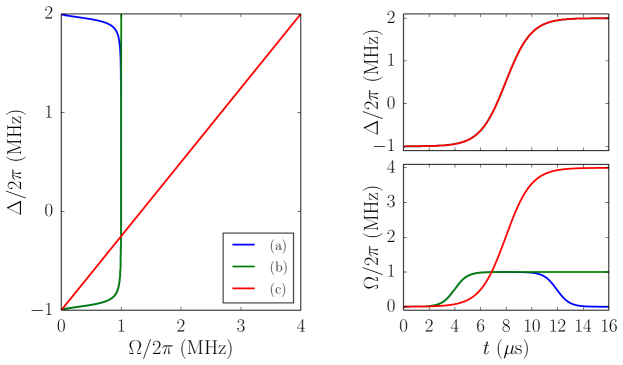
Figure 4: The three different parameter sweep paths (a), (b), (c), corresponding to the final Rabi frequencies $\Omega(t_{f})/2\pi=0,1$ and $4$ MHz. The left plot shows the three paths in parameter space, whereas the right plots show how the parameters evolve as a function of time. Initially, all atoms are in the ground state with $\Omega(t_{0})=0$ and $\Delta(t_{0})/(2\pi)=-1$ MHz.

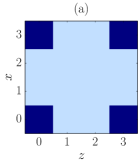
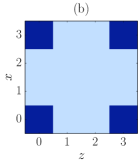
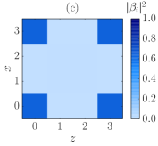
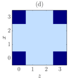
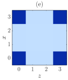
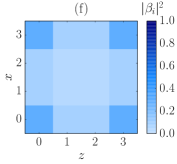
Figure 5: Comparison of TDVP with ED. Upper panel: distribution of Rydberg atoms for isotropic interactions after the three parameter sweeps shown in figure 4 using the TDVP approach. Lower panel: same as in the upper panel but calculated using ED. For small final Rabi frequencies the results obtained by both approaches are basically indistinguishable. The corresponding energies per particle are $E=0.603,0.556,0.204\,h\,$MHz for (a), (b), (c) in the upper panel and $E=0.602,0.548,-0.049\,h\,$MHz for (d), (e), (f) in the lower panel.

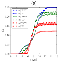
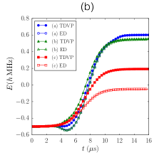
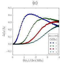
Figure 6: Comparison between TDVP and ED. (a) density of Rydberg atoms $f_{R}$ as a function time $t$ during the sweep for the three paths shown in figure 4. (b) Energy as function of sweep time. (c) graph shows the difference in the Rydberg density $\Delta f_{R}/f_{R}$ after an adiabatic parameter sweep as calculated from TDVP with respect to ED as a function of the final $\Omega(t_{f})/(2\pi)$ and for four different final detunings $\Delta(t_{f})/(2\pi)=1,2,3,4$ MHz. For $\Delta(t_{f})/(2\pi)=2$ MHz the difference $\Delta f_{R}$ of the Rydberg density between the two methods starts to deviate from zero if $\Omega(t_{f})/(2\pi)\gtrsim 1$ MHz, indicating the breakdown of our variational approach.

Figure 5 shows final distributions of Rydberg atoms computed using our TDVP approach (upper panel) as well as ED (lower panel) for the three sweeps (a) (b) (c). Note that in contrast to the 1D case, the variational ansatz describes the sweep to the classical limit $\Omega(t_{f})=0$ perfectly well, even though our approach propagates the wave-function through the non-classical region $\Omega>0$, where our ansatz is not strictly valid. In a perfectly adiabatic situation corresponding to $t_{f}\to\infty$, the final state obtained with our time-dependent variational approach would coincide with the variational ground state, which is the exact ground state in this case. The fact that our results for a finite sweep time compare very well with the exact solution suggests that deviations from adiabaticity are negligible. For such a small system size, the competition between the laser excitation and the vdW interactions results in a regular pattern of four Rydberg atoms placed at the corners of the system. We also obtain a good agreement for $\Omega(t_{f})/(2\pi)=1$ MHz and the corresponding pattern is not modified compared to the classical limit. However, for $\Omega(t_{f})/(2\pi)=4$ MHz, our ansatz overestimates the ground state energy considerably, even though the distribution of excitations looks similar to the exact result. It is also instructive to study how the system behaves during the sweep. Figure 6s (a) and (b) show a comparison of Rydberg density $f_{R}$ and energy as function of time during the parameter sweep for the three sweep protocols shown in figure 4. Again a substantial difference between TDVP and ED is only visible for sweeps to large final Rabi frequencies.

The results shown in figure 5 and figure 6(b),(c) allow to assess the validity of our approach for a realistic dynamical state preparation. We are also interested in estimating the typical value of the parameters $\Omega$, $\Delta$ where our ansatz can describe the ground state of the model (1), regardless of the details of the dynamical state preparation. To this end we consider a very large sweep time $t_{f}=150\ \mu$s to ensure that the equations of motion (7) lead to the formation of the variational ground state whereas the solution obtained with ED results in the exact ground state. We then estimate the regime of validity of the variational ground state as follows: we compute the Rydberg density at the end of the parameter sweep using both TDVP and ED and plot the relative difference of $f_{R}$ between the two approaches as a function of the final Rabi frequency $\Omega(t_{f})$ at the end of the sweep. Results are shown in figure 6(c) for four different final detunings $\Delta$. We see that for a final detuning $\Delta(t_{f})/(2\pi)=2$ MHz the difference $\Delta f_{R}/f_{R}$ starts to deviate from zero if the sweep protocol samples Rabi frequencies which are larger than $\Omega(t_{f})/(2\pi)>1$ MHz. Accordingly, for $\Delta/(2\pi)=2$ MHz our variational ansatz is correct as long as $\Omega/(2\pi)\lesssim 1$ MHz. We note, however, that this criterion was obtained for a small system and potentially depends on system size.

4.2 Isotropic Rydberg crystals

Now that we have assessed the regime of validity of our ansatz and checked in particular that it can quantitatively describe the dynamical preparation of Rydberg crystals in small two dimensional systems, let us now present our results for large system sizes where an exact numerical treatment is not possible.

We first describe the formation of Rydberg crystals in an isotropic configuration. In analogy to the experimental setup [13], we start from a circular (cookie shaped) distribution of $N=777$ ground-state atoms considering the three sweeps path shown in figure 4 keeping the other parameters of the last subsection unchanged.

Let us first comment on our choice of sweep paths (figure 4). In order to prepare a state which is as close as possible to the variational ground-state, it is particularly important to circumvent the region around the critical point $\Omega=0,\Delta=0$ [7] during the sweep into the crystalline phase. Indeed we found that the energy of the final state increases substantially if the initial negative detuning is chosen too small. On the other hand, if the initial detuning is too large, the length of the sweep path in parameter space is long and the rate of change of the parameters during the same sweep time is increasing such that the sweep becomes less adiabatic again. This is shown in figure 7 where we plot the energy of the final state obtained for $\Omega(t_{f})=0$ and $\Delta(t_{f})/(2\pi)=2$ MHz as a function of the initial detuning, for different sweep times. We found that the optimal choice of the initial detuning is $\Delta(t_{0})/(2\pi)=-1$ MHz. In this case our sweeps are almost adiabatic in the sense that the energy of the states at the end of the sweeps is less than three percent above the ground-state energy which we found by an independent optimization of the variational wave-functions using a homotopy-continuation method [38].

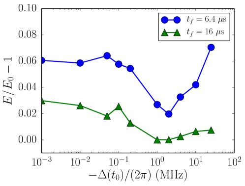
Figure 7: Influence of the sweep time $t_{f}$ and of the initial detuning $\Delta(t_{0})$ on the energy $E$ at the end of the sweep for the case of isotropic interactions and $\Omega(t_{f})=0$ and $\Delta(t_{f})/(2\pi)=2$ MHz. $E_{0}$ represents the minimum of the energy obtained for $t_{f}=16\ \mu$s and $\Delta(t_{0})/(2\pi)$= -1 MHz which corresponds to the first path in figure 4. The results show that the fidelity to stay in the ground-state during the parameter sweep decreases if $\Delta(t_{0})$ is too small or the sweep time is too short.

Results for the final distribution of Rydberg excitations at the end of the sweep are shown in figure 8. We note that for all three sweep protocols we obtain a single crystalline pattern which respects the symmetries of the cookie-shaped atom distribution. The shape of the crystal is pinned by boundary effects and the variational ground-state that we find is non-degenerate and unique. This is in contrast to experiments, where different symmetry-related, almost degenerate crystal configurations are observed from shot to shot [13]. Also note that our equations of motion for the variational parameters (7) preserve symmetries during time evolution. If degenerate, symmetry related ground states exist for a given set of parameters $\Delta$ and $\Omega$, the time evolution passes through a bifurcation point, which signals the presence of the phase transition to the crystalline state. At this point tiny numerical errors will pick out one of the degenerate ground states. It is important to emphasize, however, that we always found a unique, symmetric variational ground-state for the parameters considered here.

Ideally, the first sweep to a final Rabi frequency $\Omega(t_{f})=0$ shown in figure 4(a) prepares the ground-state of the classical Ising model, if the sweep were perfectly adiabatic. In this case the arrangement of excited Rydberg atoms would correspond to the minimum energy configuration of classical charges with a $1/r^{6}$ potential and the probability to be in the Rydberg state is either zero or one in this limit. From figure 8(a) one can see that the probability to be in the Rydberg state is $\sim 0.8$ rather than $0$ or $1$ on some sites, indicating deviations from adiabaticity. Nevertheless, a crystalline arrangement of Rydberg atoms is clearly visible. The average density of Rydberg atoms is $f_{R}=0.09$ in this case, which is in accordance with an average distance between two excitations on the order of $\left[C_{6}\left(\frac{\pi}{2}\right)/\hbar\Delta\right]^{1/6}\approx 2-3$.

For the case of sweeps to finite final Rabi frequencies $\Omega(t_{f})$ away from the classical limit [figures 8(b) and (c)], quantum superpositions between ground-state and excited atoms are present, and the probability to be in the Rydberg state is thus no longer restricted to zero or one. For increasing final $\Omega$ quantum fluctuations are stronger and the average number of Rydberg excitations increases, while the average excitation probability decreases. At large enough $\Omega$ the crystalline arrangement finally melts and one enters a quantum disordered regime where the average excitation probability is equal on all lattice sites. This trend is visible in panel (c).

Note that the complex crystalline arrangement of Rydberg atoms is strongly dependent on the size and of the shape of the system. In an infinite system the excited atoms would ideally maximize their average distance, which would result in a triangular lattice of Rydberg atoms. Due to the underlying square optical lattice strong commensurability issues arise, however, in particular if the average distance between excitations is on the order of a few lattice spacings. We observe that the crystalline structure is strongly pinned by boundary effects in our case and the crystalline structures in the classical limit thus do not resemble those which supposedly exist in the thermodynamic limit [31].

4.3 Anisotropic Rydberg crystals

We now describe the preparation of anisotropic Rydberg crystals. In this case, the magnetic field is set along the $z$-direction of the optical lattice, as shown in figure 1(a), keeping the other parameters such as sweep paths, atom distribution and the Rydberg level unchanged. Accordingly, the interaction between Rydberg atoms is anisotropic and stronger in x- than in z-direction.

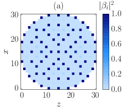
Figure 8: Distribution of Rydberg excitations at the end of the three parameter sweep protocols (a), (b), (c) shown in figure 4 for the case of isotropic interactions. Plotted is the probability $|\beta_{i}|^{2}$ to be in the Rydberg state on each lattice site. The corresponding energies per lattice site are $E=0.86,0.82,0.52\,h\,$MHz. The crystalline arrangement of Rydberg atoms is clearly visible. In the classical limit $\Omega\to 0$ (left) the excitation probabilities are close to either zero or one, whereas quantum superpositions with intermediate values of $|\beta_{i}|^{2}$ appear at finite $\Omega$ (middle, right).

Results for the three sweep paths are presented in the upper panel of figure 9. As in the isotropic case, the crystal progressively melts as $\Omega$ is increased. Note, however, that the anisotropy is visible in all cases and the crystalline structure melts first in the weakly interacting z-direction while translational symmetry is still broken in the strongly interacting x-direction. Again, we observe that the form of the Rydberg crystal is strongly pinned by boundary effects, similar to the isotropic case.

In the classical limit $\Omega=0$, we find an anisotropic crystal with an average distance between excitations on the order of $\left[C_{6}\left(\frac{\pi}{2}\right)/\hbar\Delta\right]^{1/6}\approx 3$ in the $x-$direction and of $\left[C_{6}\left(0\right)/\hbar\Delta\right]^{1/6}\approx 1-2$ in the $z-$direction. Again, the results for the sweep to the classical limit $\Omega(t_{f})=0$ indicate that the preparation was not perfectly adiabatic. Indeed, the excitation probabilities differ from 0 or 1 at the end of the parameter sweep, as in the case of isotropic interactions. The deviations from adiabaticity are even more pronounced for anisotropic interactions, as we find non-classical excitation probabilities on the order of $\sim 0.5$ in this case. This can be attributed to the fact that the excitation gaps are smaller compared to the case of isotropic interactions, due to the substantially weaker interaction in z-direction.

In order to estimate the fidelity of the dynamic state preparation scheme we plot the distribution of Rydberg atoms obtained after a direct minimization of the ground-state energy within our variational ansatz in the lower panel of figure 9. Comparing this to the distributions obtained after the parameter sweep it is apparent that a number of defects are created due to the not fully adiabatic sweep protocol. Again, the crystalline arrangement is not strongly affected by the rather short sweep time, however.

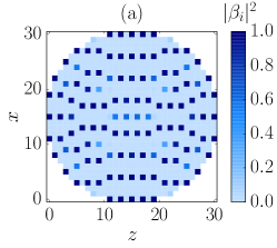
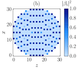
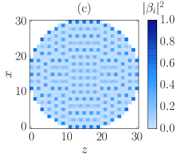
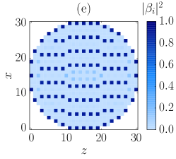
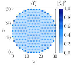
Figure 9: Upper panel: distribution of Rydberg excitations at the end of the three parameter sweep protocols (a), (b), (c) shown in figure 4 for the case of anisotropic interactions. Corresponding energies per lattice site are $E=0.79,0.74,0.30\,h$ MHz. Lower panel: distribution of Rydberg excitations obtained after a direct minimization of the variational ground-state energy. The Rabi frequencies and detunings match the parameters at the end of the sweep protocols in the upper panel. Corresponding ground-state energies per particle are $E=0.77,0.72,0.29\,h\,$ MHz. Defects in the crystalline arrangement due to the small non-adiabaticity of the sweep protocols are clearly visible in the left panel.

5 Conclusion and outlook

In the present work we have developed a time dependent mean field theory to model the dynamical preparation of anisotropic Rydberg crystals with atoms in 2D optical lattices. In addition we have presented results of numerical simulations relevant for experimentally realistic system sizes, in the limit of patterns with a large number of Rydberg excitations.

We note that the anisotropic character of the vdW interactions has been seen experimentally in a recent Rydberg-blockade experiment involving Rydberg s and d-states [39]. In contrast to the present work, where we considered the anisotropic vdW interactions between single Zeeman levels of the Rydberg states, i.e. in the limit of large Zeeman splitting, in these experiments vdW couplings involving transitions between Zeeman levels can be important. This interplay leads to several new physical phenomena, which will be presented in a future work.

References

References

- [1] Saffman M, Walker T G and Mølmer K 2010 Reviews of Modern Physics 82 2313–2363 ISSN 0034-6861 URL http://link.aps.org/doi/10.1103/RevModPhys.82.2313
- [2] Löw R, Weimer H, Nipper J, Balewski J B, Butscher B, Büchler H P and Pfau T 2012 Journal of Physics B: Atomic, Molecular and Optical Physics 45 113001 ISSN 0953-4075 URL http://stacks.iop.org/0953-4075/45/i=11/a=113001?key=crossref.12ca63182fe7b970c8c27db2e22c4fb2
- [3] Bloch I, Dalibard J and Zwerger W 2008 Reviews of Modern Physics 80 885–964 ISSN 0034-6861 URL http://link.aps.org/doi/10.1103/RevModPhys.80.885
- [4] Bloch I, Dalibard J and Nascimbène S 2012 Nature Physics 8 267–276 ISSN 1745-2473 URL http://www.nature.com/doifinder/10.1038/nphys2259
- [5] Georgescu I M, Ashhab S and Nori F 2014 Reviews of Modern Physics 86 153–185 ISSN 0034-6861 URL http://link.aps.org/doi/10.1103/RevModPhys.86.153
- [6] Robicheaux F and Hernández J 2005 Physical Review A 72 063403 ISSN 1050-2947 URL http://link.aps.org/doi/10.1103/PhysRevA.72.063403
- [7] Weimer H, Löw R, Pfau T and Büchler H P 2008 Physical Review Letters 101 250601 ISSN 0031-9007 URL http://link.aps.org/doi/10.1103/PhysRevLett.101.250601
- [8] Pohl T, Demler E and Lukin M D 2010 Physical Review Letters 104 043002 ISSN 0031-9007 URL http://link.aps.org/doi/10.1103/PhysRevLett.104.043002
- [9] Schachenmayer J, Lesanovsky I, Micheli A and Daley A J 2010 New Journal of Physics 12 103044 URL http://stacks.iop.org/1367-2630/12/i=10/a=103044
- [10] Lesanovsky I 2011 Physical Review Letters 106 025301 ISSN 0031-9007 URL http://link.aps.org/doi/10.1103/PhysRevLett.106.025301
- [11] Gärttner M, Heeg K P, Gasenzer T and Evers J 2012 Physical Review A 86 033422 ISSN 1050-2947 URL http://link.aps.org/doi/10.1103/PhysRevA.86.033422
- [12] SchaußP, Cheneau M, Endres M, Fukuhara T, Hild S, Omran A, Pohl T, Gross C, Kuhr S and Bloch I 2012 Nature 491 87–91 ISSN 1476-4687 URL http://www.nature.com/nature/journal/v491/n7422/full/nature11596.html#supplementary-information
- [13] SchaußP, Zeiher J, Fukuhara T, Hild S, Cheneau M, Macrì T, Pohl T, Bloch I and Gross C 2014 10 (Preprint 1404.0980) URL http://arxiv.org/abs/1404.0980
- [14] Jaksch D, Cirac J I, Zoller P, Rolston S L, Côté R and Lukin M D 2000 Phys. Rev. Lett. 85 2208–2211 URL http://link.aps.org/doi/10.1103/PhysRevLett.85.2208
- [15] Lukin M D, Fleischhauer M, Cote R, Duan L M, Jaksch D, Cirac J I and Zoller P 2001 Phys. Rev. Lett. 87 37901 URL http://link.aps.org/doi/10.1103/PhysRevLett.87.037901
- [16] Tong D, Farooqi S M, Stanojevic J, Krishnan S, Zhang Y P, Côté R, Eyler E E and Gould P L 2004 Physical Review Letters 93 063001 ISSN 0031-9007 URL http://link.aps.org/doi/10.1103/PhysRevLett.93.063001
- [17] Singer K, Reetz-Lamour M, Amthor T, Marcassa L G and Weidemüller M 2004 Physical Review Letters 93 163001 ISSN 0031-9007 URL http://link.aps.org/doi/10.1103/PhysRevLett.93.163001
- [18] Cheinet P, Trotzky S, Feld M, Schnorrberger U, Moreno-Cardoner M, Fölling S and Bloch I 2008 Physical Review Letters 101 090404 ISSN 0031-9007 URL http://link.aps.org/doi/10.1103/PhysRevLett.101.090404
- [19] Gaëtan A, Miroshnychenko Y, Wilk T, Chotia A, Viteau M, Comparat D, Pillet P, Browaeys A and Grangier P 2009 Nature Physics 5 115–118 ISSN 1745-2473 URL http://www.nature.com/doifinder/10.1038/nphys1183
- [20] Urban E, Johnson T a, Henage T, Isenhower L, Yavuz D D, Walker T G and Saffman M 2009 Nature Physics 5 110–114 ISSN 1745-2473 URL http://www.nature.com/doifinder/10.1038/nphys1178
- [21] Weimer H and Büchler H P 2010 Physical Review Letters 105 230403 ISSN 0031-9007 URL http://link.aps.org/doi/10.1103/PhysRevLett.105.230403
- [22] Sela E, Punk M and Garst M 2011 Physical Review B 84 085434 ISSN 1098-0121 URL http://link.aps.org/doi/10.1103/PhysRevB.84.085434
- [23] Höning M, Muth D, Petrosyan D and Fleischhauer M 2013 Physical Review A 87 023401 ISSN 1050-2947 URL http://link.aps.org/doi/10.1103/PhysRevA.87.023401
- [24] Lesanovsky I and Garrahan J P 2013 Physical Review Letters 111 215305 ISSN 0031-9007 URL http://link.aps.org/doi/10.1103/PhysRevLett.111.215305
- [25] Petrosyan D 2013 Physical Review A 88 043431 ISSN 1050-2947 URL http://link.aps.org/doi/10.1103/PhysRevA.88.043431
- [26] Hoening M, Abdussalam W, Fleischhauer M and Pohl T 2014 1–5 (Preprint arXiv:1404.1281v1)
- [27] Reinhard A, Liebisch T, Knuffman B and Raithel G 2007 Physical Review A 75 032712 ISSN 1050-2947 URL http://link.aps.org/doi/10.1103/PhysRevA.75.032712
- [28] Glaetzle A W, Dalmonte M, Nath R, Rousochatzakis I, Moessner R and Zoller P 2014 1 26 (Preprint 1404.5326) URL http://arxiv.org/abs/1404.5326
- [29] Beterov I, Ryabtsev I, Tretyakov D and Entin V 2009 Physical Review A 79 052504 ISSN 1050-2947 URL http://link.aps.org/doi/10.1103/PhysRevA.79.052504
- [30] Glaetzle A, Nath R, Zhao B, Pupillo G and Zoller P 2012 Physical Review A 86 043403 ISSN 1050-2947 URL http://link.aps.org/doi/10.1103/PhysRevA.86.043403http://journals.aps.org/pra/abstract/10.1103/PhysRevA.86.043403
- [31] Rademaker L, Pramudya Y, Zaanen J and Dobrosavljević V 2013 Physical Review E 88 032121 ISSN 1539-3755 URL http://link.aps.org/doi/10.1103/PhysRevE.88.032121
- [32] Bak P and Bruinsma R 1982 Physical Review Letters 49 249–251 URL http://prl.aps.org/abstract/PRL/v49/i4/p249_1
- [33] Lee S, Lee J R and Kim B 2001 Physical Review Letters 88 025701 ISSN 0031-9007 URL http://link.aps.org/doi/10.1103/PhysRevLett.88.025701
- [34] Zeller W, Mayle M, Bonato T, Reinelt G and Schmelcher P 2012 Physical Review A 85 063603 ISSN 1050-2947 URL http://link.aps.org/doi/10.1103/PhysRevA.85.063603
- [35] Kramer P 2008 Journal of Physics: Conference Series 99 012009 ISSN 1742-6596 URL http://stacks.iop.org/1742-6596/99/i=1/a=012009?key=crossref.1c90eeaaf0c5688a83779f1c8c82dd9d
- [36] Walker T and Saffman M 2008 Physical Review A 77 032723 ISSN 1050-2947 URL http://link.aps.org/doi/10.1103/PhysRevA.77.032723
- [37] Marinescu M, Sadeghpour H and Dalgarno A 1994 Physical Review A 49 982–988 ISSN 1050-2947 URL http://link.aps.org/doi/10.1103/PhysRevA.49.982
- [38] Punk M 2014 5 (Preprint 1405.5894) URL http://arxiv.org/abs/1405.5894
- [39] Barredo D, Ravets S, Labuhn H, Béguin L, Vernier A, Nogrette F, Lahaye T and Browaeys A 2014 Phys. Rev. Lett. 112 183002 URL http://link.aps.org/doi/10.1103/PhysRevLett.112.183002